Spatial Autocorrelation and Bayesian Spatial Statistical Method for Analyzing Intersections Prone to Injury Crashes Sudeshna Mitra rates; nevertheless, many cities and DOTs still use these simplified techniques to rank high-crash-risk road segments, ramps, and intersections for further improvements. A possible explanation of this ongoing practice could be the complexity of all of these mathematical techniques, which require special training and skills in statistical analysis; these requirements often prevent the implementation of these superior methodologies in practice. Additionally, these approaches are not generally combined with any visual tool or mapping software that could help in displaying the outcomes (i.e., physical locations of high concentrations of collisions of these techniques). As a result, these sound and appropriate methodologies have often been underused by cities and DOTs, which are still dependent on their in-house tools—which may not be particularly accurate and sophisticated— to allocate their limited resources to make important decisions about ranking high-crash-risk locations and thereby improving that DOT’s overall safety profile. Another drawback is that many DOTs do not maintain a geographic information system (GIS) crash database, which means they are unable to perform any GIS-based crash mapping to detect high-crash-concentration locations on their road networks. Though GIS-based methods may or may not be as superior as the EB method, they are at least better than methods that use crash counts or crash rates. Moreover, if overlaid with other layers, GIS-based mapping could help to associate high-crash locations with spatial factors. In transportation safety applications, GIS has been widely used to geocode accident locations, developing pin maps of crashes and database queries as performed by Levine et al. (11, 12), Affum and Taylor (13), Austin et al. (14), Kim and Levine (15), and Miller (16). However, some researchers (11, 12, 16–22) have incorporated some of the powerful analytical tools available in GIS software (e.g., buffer, nearest-neighbor method, simple density, and the kernel density estimation method of crash cluster detection) to show spatial distribution of crashes at the road-network level. Another powerful analytical tool available in commercial GIS software but often underused in transportation safety is the spatial statistical toolbox. If public agencies do not have their crash database in a GIS platform, however, they will be unable to use some of these powerful yet straightforward statistical analysis tools available in GIS. Another drawback of not using GIS in the detection of crash hot spots is the possibility of ignoring important spatial-location-specific information that might have a strong effect on crash occurrence. For example, spatial features near a road network might influence the frequency of crashes at a particular location, which would be hard to detect without the use of a tool such as GIS. Some recent studies have demonstrated the relevance and usefulness of the spatial statistical analysis tools available in commercial GIS software to investigate any association of crashes with spatial features of interest in a transportation network.
Identification of hazardous road locations (i.e., crash hot spots or black spots) is a standard practice in departments of transportation (DOTs) throughout the United States. Often, DOTs use relatively straightforward methods to detect high crash sites; these methods, however, may not be accurate. The objectives of this study are to develop two different methodologies: (a) a geographic information system (GIS)-based method to detect crash hot spots and (b) a spatial regression method with structured and unstructured random effects in continuous space to investigate the intersection-level factors that influence the concentration of fatal injury crashes. Using injury and property damage only (PDO) crash data from Tucson, Arizona, this study shows that spatial dependence plays a strong role during the analyses of road-traffic crashes. These spatial dependencies, accounted through spatial autocorrelation, help to detect statistically significant clusters of crashes involving fatalities or severe or minor injuries, in a GIS framework. This study also develops statistical models of severe- and minor-injury crashes, using classical negative binomial (NB) and Bayesian spatial statistical methods incorporating spatially structured and unstructured random effects. The coefficient estimates from a Bayesian framework are similar to those from NB estimation, but with better precision. The model that includes spatial correlations also indicates the potential to reduce the bias associated with model misspecification by changing the estimate of the annual average daily traffic coefficients. This study’s results also indicate that spatially structured correlation is quite significant in cases of crashes involving minor injury or PDO and that unstructured effects are somewhat significant at the intersection-level for cases of severe-injury crashes.
Identifying crash hot spots, black spots, high risk, or high-collisionconcentration locations is a standard practice in departments of transportation (DOTs) throughout the United States, to ensure the efficient allocation of the available safety funds to reduce crash frequencies and severities. A fair amount of literature has been focused on methods for identifying hot spots through the use of advanced statistical methods such as the empirical Bayes (EB) technique (1–6), full Bayes methodology (7, 8), simulation methodology (9) and other innovative methods (10). It is generally accepted by safety researchers that the EB technique outperforms simplified methods of crash hotspot detection, especially methodologies that use crash counts or crash
Civil and Environmental Engineering Department, California Polytechnic State University, 1 Grand Avenue, San Luis Obispo, CA 93407.
[email protected]. Transportation Research Record: Journal of the Transportation Research Board, No. 2136, Transportation Research Board of the National Academies, Washington, D.C., 2009, pp. 92–100. DOI: 10.3141/2136-11
92
Mitra
For example, Flahaut et al. (23) used two different spatial statistical techniques, a global autocorrelation index and kernel estimation, to identify clusters of road-segment crashes in Belgium. In addition, Qin (24) used the hotspot analysis tools available in GIS to locate snow-related crash locations, and Bejleri et al. (25) used customized methodologies in GIS to locate road segments and intersections with high concentrations of pedestrian- and bicycle-related crashes. In addition to noting that by not using GIS possible associations of spatial physical and environmental factors may be missed, it is also important to mention that few studies have considered the effect of spatial site-specific factors in detecting hazardous road locations. While the EB method is considered a better method to use to detect hazardous sites, researchers often consider the characteristics of a location, mostly through traffic volumes and sometimes through geometric design properties. Although traffic volume is considered the single most important exposure variable, it is also well known that spatial-location-specific factors help to explain unobserved heterogeneity in crash data. For example, Bauer and Harwood (26) showed that traffic-volume-related variables could capture from 16% to 38% of the variability in crashes, leaving a small (from 5% to 14%) portion of the variability explained by geometric design variables. However, the unexplained variability (about 40% in this case) could be attributed to both structured as well as unstructured error terms. In another study, Griebe (27 ) developed prediction models for both road links and junctions and showed that the road-link model could capture more than 60% of the systematic variation and that the intersection model had lower explanatory power. Chin and Quddus (28) confirmed that traffic volumes are the most important factor, or main effect, in predicting crashes. Although these studies concluded that traffic volume is the primary indicator variable, such researchers as Ivan et al. (29), Ossenbruggen et al. (30), and Aguero-Valverde and Jovanis (31) have examined the effect of spatial factors on roadsegment crashes. Wang and Abdel-Aty (32) have examined this effect on intersection-related rear-end crashes, and Karlaftis and Tarko (33), Noland and Quddus (34), and Aguero-Valverde and Jovanis (35) have examined this effect on county-level crashes. Few (if any) studies, however, have focused on modeling crash severities at intersections to check if spatial site-specific correlations have any influence in detecting high injury crash locations. The omission of spatial sitespecific characteristics could lead to erroneous identification of crash hot spots or black zones because in such cases spatial autocorrelation is ignored. The concept of spatial autocorrelation is important when specific attributes of a variable tend to have interdependence over space. This phenomenon holds true in cases of crash hot spots or black zones, which have high frequencies of crashes as well as higher concentrations of certain types, maneuvers, or other specific attributes of crashes that are observed and tend to get overrepresented. In such cases, important information would be lost if spatial dependence of crashes was ignored. With this background, the current study has two primary objectives: 1. To demonstrate a GIS-based methodology for detecting crash hot spots through the use of the spatial statistical analysis tools available in GIS and 2. To develop a Bayesian spatial statistical method to investigate whether spatial factors have any influence on the occurrence of injury crashes at the intersection level. The first of these objectives is intended to provide practitioners in the transportation field with a straightforward yet important tool to detect statistically significant crash clusters; the second objective is
93
aimed at developing an advanced technique to investigate whether spatially structured intersection-specific effects have any significant influence in explaining the occurrence of clusters of crashes involving fatalities and injuries. Therefore, this study is important both from a practical viewpoint and as a long-term contribution to transportation safety literature. In the following sections, the theory and methodology of crash hotspot detection in a GIS framework is described first, followed by a discussion of the theory and methodology of the Bayesian framework of crash modeling. These two methodologies are then applied to data on intersection-related crashes within the city of Tucson, Arizona. Finally, conclusions from this study as well as possible future research topics are discussed. A separate section for literature review is not provided in this paper because the relevant literature is cited and discussed in appropriate sections of this paper.
IDENTIFICATION OF SPATIAL CONCENTRATION OF CRASHES USING GIS There are several analytical tools available in GIS to analyze point features such as road-traffic crash occurrence. Two of the common point-pattern detection tools available in GIS are (a) quadrant analysis or the density analysis tool and (b) the nearest-neighbor analysis tool. In recent years, Schneider et al. (21) used the nearest-neighbor method to detect clusters of pedestrian crashes. The authors developed standard deviational ellipses of each of the nearest-neighbor clusters and the number of points these ellipses contain to measure the dispersion and orientation of the points around the mean center of the clusters. Pulugurtha et al. (22) utilized the concept of quadrant or grid-based analysis to compute crash density and concentration as a measure for detecting crash hot spots. The authors used two different techniques of density estimation: the simple density computation method and a method that uses the kernel density estimation tools available in the ArcGIS toolbox. As expected, the kernel density methodology provided greater accuracy in hotspot detection due to its sophisticated mathematical algorithm, in contrast to the simple density computation method. After computing the densities, these researchers developed a composite score for ranking high-crash locations by combining three different methods: crash frequency, crash density, and crash rates. Sando et al. (36) also utilized a nearestneighbor algorithm to detect crash patterns and compared the merits of this methodology with other statistical techniques such as regression analysis, neural network, and Bayesian techniques. These authors suggested that in the absence of a priori knowledge about probability distribution of the count patterns, the nearest-neighbor technique is quite effective. Although density analysis and nearest-neighbor analysis are commonly used in point-pattern detection, both density and nearestneighbor analyses treat all points (in this case, crashes) as if they are the same. In other words, these two methods analyze only the location, and not the attributes, of a point. Spatial statistical tools, on the other hand, take into account both the location of the crash and that location’s attributes. As a result, these are considered more powerful tools because they account for both the location of the crash and the activities occurring at that particular location. Specifically, spatial autocorrelation analysis assesses the extent to which the value of a variable X at a given location i is related to the values of that variable at contiguous or neighboring locations. Hence the basic concept of spatial autocorrelation is related to the interdependence of a specific attribute over space. Clearly, this is the main idea behind investigating locations of high crash concentrations: to identify locations with
94
Transportation Research Record 2136
unusually high numbers of specific types of crashes. The assessment of spatial correlation involves analyzing the degree to which the value of a variable for each location co-varies with values of that variable at nearby locations (23). When the level of co-variation is higher than expected, contiguous locations have similar values and autocorrelation is positive. When the level of co-variation observed is negative, high values of the variable are contiguous with low values and the autocorrelation is negative. The lack of a significant positive or negative co-variation suggests the absence of spatial autocorrelation. To quantify the spatial correlation, two popular indices are generally used: Geary’s ratio and Moran’s I. These are known as global methods of assessing spatial autocorrelation, and they measure and test for whether patterns of point distributions are clustered or dispersed in space with respect to their attribute values. In this context, it is important to note that both Geary’s ratio and Moran’s I measure autocorrelation for interval or ratio data. Most analysts favor Moran’s I because its distributional characteristics are more desirable and the index has greater general stability and flexibility. Moran’s I index is defined as
∑ ∑ w ( x − x )( x I= s ∑∑w ij
i
i
j
j
− x)
Ii = ( xi − x ) ∑ wij ( x j − x ) i
Similar to the global Moran’s I, a high value of the local Moran’s indicates clustering of similar values, and a low value means a clustering of dissimilar values of a variable. The cluster analysis tool available in GIS provides estimation of local Moran’s values and the associated Z-scores for all locations in the study area. The Z-score represents the statistical significance of the index value: that is, whether the apparent similarity (or dissimilarity) in values between the feature and its neighbors is greater than would be expected to occur simply by chance. A high positive Z-score for a feature indicates that the surrounding features have similar values and helps to find locations with specific types of crash concentration. A low negative Z-score for a feature indicates the feature is surrounded by dissimilar values. Once these Z-scores are calculated, it is possible to identify statistically significant spatial locations with high concentrations of crashes.
INVESTIGATION OF SPATIAL DEPENDENCIES OF CRASHES USING BAYESIAN MODELING
2
ij
i
j
where wij = weights representing proximity relationships between location i and neighboring location j; xi = value of the interval or ratio variable X at location i; –x = mean of all x ’s; i n = total number of locations, i = 1, 2, . . . , n and j = 1, 2, . . . , n; and 2 ∑ ( xi − x ) i 2 s = n = measure of sample variance. In cases of point-pattern detection, generally the weight wij is used as the inverse of the distance between two points i and j. This is derived from first law of geography, which suggests larger weights to points that are close and smaller weights to points that are far apart. Hence wij is generally defined as 1/d δij, where δ may be taken at any appropriate value such as 0.5, 1.0, 1.5, 2.0 or any other number based on specific characteristics or empirical evidence associated with the geographic phenomena in question. Many empirical studies (37 ) in spatial autocorrelation have shown that a δ value of 2.0 for the exponent of distance indicates a stronger reduction in the importance of the points located further away, making spatial association stronger with closest neighbors. Hence a widely acceptable value of δ = 2.0 has been adopted in this study. The major difference between Geary’s ratio and Moran’s I is that in Geary’s ratio the numerator consists of the square of the difference in attribute values for point i and point j such that (xi − xj )2 is considered instead of the measure (xi − –x )(xj − –x ) as in the case of Moran’s I. Although this global method for assessing spatial autocorrelation has existed for longer, there are also local indicators of spatial association such as the local version of Moran’s I proposed by Anselin (38). This index is used to indicate the level of spatial autocorrelation at the local scale (i.e., a value of the index is calculated for each spatial unit i). The local Moran’s statistic for unit i is defined as
While the previous section focused on the importance of a spatial statistical tool and illustrated how that tool could be applied to detect high concentrations of a specific type of crash using the readily available tools in GIS, this section focuses on the Bayesian modeling of crash events to discover spatial factors that influence certain types of crash concentrations at signalized intersections. The reason behind the increasing interest in investigating spatial and temporal factors affecting traffic crashes is that many of the factors that influence crashes operate in a spatial scale. In recent studies, Wang and Abdel-Aty (32), Aguero-Valverde and Jovanis (31, 35), and Mitra et al. (39) have shown that spatial factors have a strong influence on crash occurrences. In this study, spatial statistical modeling is used to detect if certain spatial locational factors influence spatial concentration of injury and fatal crashes. This study has adopted a Bayesian statistical inference because this approach plays a major role in developing statistical inference of spatial data from both discrete and continuous perspectives. Although the application of discrete spatial statistics is primarily used in the field of disease mapping to estimate underlying pattern of relative risk, Bayesian spatial statistical inference has been used widely in recent years (31, 35, 40, 41) in road-traffic crash mapping because crashes and disease events have similar properties and natures. The risks of traffic crashes vary within areas as well as among areas because site-related spatial and temporal (both observed and unobserved) factors influence crash occurrences. If it is included, spatial information can capture significant heterogeneity that leads to extra variation in crash data. This extra variation can be modeled by including random effects in a model for the relative risks of crashes. Some effects may be spatially unstructured and generally denoted as excess heterogeneity. However, overdispersion may also occur due to spatially correlated effects. Such spatial effects often proxy unobserved risk factors, which vary over space (42). A hierarchical Bayesian modeling is appropriate in such cases and is adopted for this study. The model is given as yi ~ Poisson ( μ i ) where yi is the observed count of crashes and µi is the expected number of crashes at road location i. In this case road location is
Mitra
95
intersection, so expected crash counts are proportional to entering traffic volume. The relative risk is modeled as log ( μ i ) = β1 + β 2 xi 2 + . . . + βxi + si + ui
Data Set
where xi β si ui
= = = =
based spatial statistical tools and the application of Bayesian framework to detect spatial association and of the findings from the use of these methodologies.
explanatory variables or covariates, fixed effect parameters, spatially structured effects or spatial correlations, and spatially unstructured errors or the uncorrelated heterogeneities with a prior, ui ∼ N(0, τ 2u ), where τ u2 is assigned a gamma prior.
β is assigned to noninformative normal priors. While the spatially structured effects si are assumed to follow a conditional autoregressive model in case of discrete areas, a different geostatistical model with MCMC sampling is generally followed in case of observations at points in continuous space (42). As the locations of interest in this study are intersections, the geostatistical model with joint rather than conditional prior for spatial effects is used in this study. As proposed by Banerjee et al. (43), these models take the effect of proximity and directions of the points to develop the covariance matrix and joint prior, which is multivariate normal and can be written as P ( s1 , s2 , . . . , sn ) ~ N ( 0, Σ ) where Σ = σ 2s R and R = [rij] = exp[−(φdij)δ]. The spatial dependence between points xi and xj is separated by distance dij, which follows a spatial exponential form. Similar to the unstructured case, τ 2s is assigned a gamma prior such as Ga(1, 0.001). Also, τ 2s = 1/σ 2s and τ 2u = 1/σ 2u are known as precision and η = 1/ϕ is called the range and defines the distance dij where the correlation between xi and xj is zero or effectively zero. This geostatistical modeling is performed using the WinBUGS software package (44). The results from both GIS and WinBUGS analyses are discussed in detail in the following section along with a brief description of data set used for this study.
APPLICATION OF METHODOLOGY TO DETECT HIGH CRASH INTERSECTIONS The methodologies described in the previous sections are applied to detect crash concentrated locations at signalized intersections in Tucson. Although the focus of the GIS-based methodology is the detection of locations with high concentrations of injury and fatal crashes, the methodology could be applied to detect any other crash types. The following sections first describe the data used in this study, which is followed by discussions of the application of GIS-
TABLE 1
Data used in this study were obtained from two different sources: (a) crash data and (b) traffic volume or exposure data. The sites examined in the study are signalized intersections in the city of Tucson. Intersection types were signalized intersections including four-legged and T-junctions; the unavailability of traffic-volume data restricted the sample to 291 signalized intersections. The nature of the two data sources is now described.
Crash Data The crash data for this study were obtained from the Accident Location Identification Surveillance System (ALISS) database maintained since 1975 by the Arizona Department of Transportation. The ALISS database contains all of the microlevel information about crashes, such as the type of crash, its severity, the time it occurred, its location and a description of that site, vehicle maneuvers before the crash, direction of movement of the vehicle before the crash, information about the people (both drivers and passengers) involved in the crash, and information on the vehicles involved. For this study, data on crashes that occurred from 2001 to 2004 at 291 signalized intersections in Tucson were collected and analyzed. Crashes were categorized as intersection-related crashes if they occurred within the curb-line limits of the intersection or if they occurred within the influence area of the intersection (which was defined as within 250 ft along any leg of the intersection from the intersection center point). A summary of various crash types is shown in Table 1; only fatal, severe-injury, and minor-injury crash data were used in this study.
Traffic Data Traffic data for this study were provided by the City of Tucson. Acquiring traffic-volume data was a major challenge. An ideal way to model crash data is to obtain the crash and traffic-volume data by year; however, for many of these sites, it proved difficult to obtain annual traffic-volume data for more than one year. Practically, this means that some hypothetical site 1 might have traffic-volume counts for 2001 but not for 2002 or 2003, whereas site 2 might have counts for 2002 but not for 2001 and 2003. Therefore, calculations based on 1 year of traffic-volume data were applied for the analysis, with all acknowledged limitations of this approach. No other data were used in this study since the goal was to check if spatial-location-related factors have any effect on crash occurrence.
Summary Statistics for Intersection Crashes and Traffic Volume
Variable
Variable Description
Mean
SD
Maximum
Minimum
SevInjCrash MinInjCrash ADTMAJ
Total severe and fatal injury crashes Total minor injury and property damage only crashes Average daily traffic from major-road
3.266 68.385 31,511.892
2.469 46.190 13,457.927
14 232 66,364.29
1 13 1,617.86
ADTMIN
Average daily traffic from minor-road
13,704.486
11,275.519
49,296.43
0.00
96
Transportation Research Record 2136
Spatial Statistical Method in GIS To examine the spatial pattern of crashes, this study focused on crashes that involved fatalities or severe or minor injuries, rather than on the total number of crashes. As mentioned earlier, the spatial autocorrelation method is an advancement over quadrant or nearestneighbor methods of spatial-pattern detection, because spatial autocorrelation not only accounts for the location of points but also for the attributes of those locations. As a result, this is a useful technique to detect locations with a higher than average probability of an injuryrelated crash occurring: crashes that are a huge economic burden for any jurisdiction. To perform this task, spatial autocorrelation coefficient using Moran’s I index and associated Z-score are computed
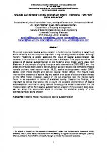
for fatal and injury crashes. As mentioned already, a high positive Z-score for a feature indicates that the surrounding features have similar values. Hence the locations where fatal and injury crashes have Z-scores of ≥2 are locations with statistically significant crash clusters at the α = 0.05 level. These intersections are extracted from the original analysis and are displayed in Figure 1. From this figure, it is quite clear that there are four main regions in Tucson—the northern, eastern, middle, and southern parts of the city—where there were concentrations of crashes involving fatality and injury. There are only seven intersections with statistically significant clusters of fatal crashes, even though 21 intersections in Tucson had one or more fatal crashes over a 3-year period. This indicates that these seven (out of the 21) intersections are most likely associated with some
Minor Injury Clusters Severe Injury Clusters Fatal Crash Clusters All Intersections 0 5,00010,000
FIGURE 1
20,000
30,000
40,000 Feet
Distribution of fatal and injury crash clusters.
Street Network
Mitra
97
inherent risk, which needs to be investigated for site improvement. Figure 1 illustrates that two of these clusters of fatal crashes coincide with clusters of severe-injury crashes; in addition, two other intersections with clusters of fatal crashes are observed to be also at high risk for both severe-injury and minor-injury crashes. The other three intersections are solely identified for their high concentration of fatal crashes and not so much for severe- or minor-injury crashes. When looking for locations of clusters of severe- and minor-injury crashes, it is observed that out of a total of 239 intersections, 59 and 61 have statistically significant crash clusters for, respectively, severe-injury and minor-injury crashes. Figure 1 also indicates that not all severeinjury crash clusters coincide with minor-injury crash clusters or vice versa. Hence, there must be some factors related to traffic, geometric design, or spatial site, which influence these outcomes. To investigate these factors, the spatial Bayesian statistical model as well as count models such as negative binomial (NB) models are applied and tested. The results from these two types of models are compared to check the influence and existence of spatial factors in crash-cluster detection.
NB and Spatial Statistical Model for High Crash Intersections Two different types of models are developed in this study. An ordinary count model using NB is developed followed by a Bayesian spatial hierarchical model with structured and unstructured error terms. The NB models are developed in STATA statistical software and the results from these models are shown in Table 2. In the case of the Bayesian analysis, all models are estimated using one chain taken to 10,000 iterations. The models are slow when spatially structured effects are included through spatial exponential function, but show early convergence, which is checked by trace plots available in WinBUGS. In this study, the samples for posterior analysis were taken after 1,000 burn-ins. The priors for regression coefficients are taken as N(0, 0.001) and that for variance terms are taken as Ga(1, 0.001) in WinBUGS modeling software where 0.001 is the precision of the distribution indicating that the variance is high (i.e., they are noninformative or flat priors). The x–y coordinates of the intersections are generated from GIS mapping and are used as model inputs to calculate the distance between any two points, and are ultimately used in computing spatial correlation. In this context, it is important to point out that intersection-level spatial correlation is as important as area- or corridor-based spatial correlation. As pointed out by Wang and Abdel-Aty (32), signalized intersections along a certain corridor,
TABLE 2
especially for those near one another, will influence each other in many aspects. In general, this spatial correlation is a function of the distance between the intersections: the closer they are, the higher the correlation will be (and vice versa). A reasonable range for the correlation rij could be computed at the observed minimum distance d1 = min(dij ) and at the observed maximum distance d2 = max(dij ) between observations. Once the minimum and maximum distances are known, a uniform prior for ϕ is chosen in such a way that the correlation at the minimum distance is approximately 1 and that at the maximum distance is approximately zero. In this study a uniform prior of U(0.1, 5) and U(0, 2) are taken for ϕ and δ, respectively, and on the basis of the estimate of ϕ the range η = 1/ϕ is computed in the model. The results from the Bayesian models are given in Table 3. For classical as well as Bayesian modeling purposes, traffic volumes from major and minor roads are the only variables considered in the mean function. No other variables (e.g., geometric or spatiallocation-related factors) are included in model building. This is done to check if traffic volume(s)—which are commonly the only factors used in identifying black spots, hot spots, or hazardous locations— are sufficient in capturing the unexplained heterogeneity in crash data. From the NB model findings (Table 2) it is clear that overdispersion is significant (i.e., there are unexplained factors in the models that could be due to structured or unstructured heterogeneity). This will be investigated later in a spatial statistical model in a Bayesian framework. In terms of the coefficient estimates, the results from severe-injury and minor-injury [including property damage only (PDO) crashes] crash modeling did not have much variation, indicating that the constant terms as well as the traffic volumes from major and minor roads are all significant in explaining the occurrence of injury crashes. When these models are tested in a Bayesian framework with structured and unstructured error terms, similar estimates are obtained but with better precisions. A closer look at results in Table 3 shows that estimates from the Bayesian models are along the same direction as those of the NB models. A comparison between coefficient estimates from the Bayesian and NB models, however, shows a distinct reduction of the estimates of annual average daily traffic (AADT) coefficients in the case of the spatial models. In addition, it is observed that all of the coefficient estimates in the Bayesian framework have lower standard errors than do the NB model estimations: a clear improvement in model estimation. To investigate the influence of structured and unstructured effects, models with variances σ 2s and σ 2u are tested for both minor-injury and severe-injury crashes. The model findings show that σ 2u is not significant and the impact is lower than σ2s in cases of minor-injury crashes, indicating that uncorrelated heterogeneity
Negative Binomial Estimation Results from Minor Injury (including PDO) and Severe Injury Crashes Models Minor Injury (including PDO) Crash
Variable Constant Log(AADTMAJ) Log(AADTMIN) Dispersion parameter α Log likelihood at zero Log likelihood at convergence NOTE: PDO = property damage only.
Estimated Coefficient −5.71 1.379 0.901 0.219 −418.057 −395.10
SD 1.308 0.244 0.152 0.035
Severe Injury Crash p-Value
Estimated Coefficient