Automata Theory Based Approach to the Join Ordering Problem in Relational Database Systems
Miguel Rodríguez1, Daladier Jabba1, Elias Niño1, Carlos Ardila1 and Yi-Cheng Tu2
1
Department of Systems Engineering, Universidad del Norte, KM5 via Puerto Colombia, Barranquilla, Colombia 2 Department of Computer Science and Engineering, University of South Florida, Tampa, USA {erodriguezm, djabba, enino, cardila}@uninorte.edu.co,
[email protected]
Keywords:
automata theory, query optimization, join ordering problem.
Abstract:
The join query optimization problem has been widely addressed in relational database management systems (RDBMS). The problem consists of finding a join order that minimizes the time required to execute a query. Many strategies have been implemented to solve this problem including deterministic algorithms, randomized algorithms, meta-heuristic algorithms and hybrid approaches. Such methodologies deeply depend on the correct configuration of various input parameters. In this paper, a meta-heuristic approach based on the automata theory will be adapted to solve the join-ordering problem. The proposed method requires a single input parameter that facilitates its usage respect to those previously described in the literature. The algorithm was embedded into PostgreSQL and compared with the genetic competitor using the most resent TPC-DS benchmark. The proposed method is supported by experimental results achieving up to 30% faster response time than GEQO in different queries.
1
INTRODUCTION
Since the early days of RDBMS the problem of finding a join order to minimize the execution time of a query has been approached. (CHAUDHURI, 1998) defined large join queries as relational algebra queries with N join operations involving N+1 relations when N is greater or equals to 10. Consecutively the Large Join Query Optimization Problem (LJQOP) was formally addressed as finding a Query Execution Plan (QEP) with a minimum cost for a large join query. The LJQOP have been widely addressed and many methods have been developed to solve it. Randomized algorithms such as iterative improvement and simulated annealing, evolutionary algorithms such as genetic algorithms and Meta heuristics such as ant colony optimization are some common strategies used in the solution of the problem. The solution space of a LJQOP consists of all query trees that answers the query. There are three types of query trees that can result from the solution space: left deep, bushy and right deep. An extended
discussion about types of query trees is given in (IOANNIDIS and KANG, 1991). The construction of a LJQOP solution space is theoretically possible for a small number of relations. When N increases substantially, finding the optimal join order is considered an NP-hard problem and thus deterministic algorithms cannot find a solution easily. Systems holding workloads from applications such as decision support systems and business intelligence require the ability of joining more than 10 relations easily. In this paper, a Meta heuristic approach based on the automata theory that has been effectively used in the solution of the Traveling Salesman Problem (TSP) will be presented and its application in the solution of the join ordering problem will be discussed. Finally the automata based query optimizer proposed in this work will be tested using the most recent decision support benchmark TPC-DS. The remaining parts of this work will be distributed as follows. Previous work on solving the LJQOP is discussed in section two. The proposed methodology will be explained in section three. The experimental design and setup used to test the algorithm is going to be exposed in section four. A
discussion about the results obtained by the algorithm and a comparison analysis between the proposed method and the PostgreSQL genetic optimizer module is showed in section five. Finally conclusions and future work are presented.
2
RELATED WORK
The join ordering problem has been approached in different ways among the years. A literature review presented in (STEINBRUNN, MOERKOTTE and KEMPER, 1997) provides detailed information on different approaches to the solution of the problem and classifies them in four groups. The first one corresponds to deterministic algorithms such as dynamic programming and minimum selectivity algorithm. The second group, randomized algorithms, includes simulated annealing, iterative improvement, two-phase optimization and random sampling. The third group consists of genetic algorithms, which encode the solutions and then uses selection, crossover and mutation algorithms. Finally the fourth group is compound of hybrid methods. Three of the most popular approximate solutions to the join-ordering problem are simulated annealing, genetic algorithms and ant colony optimization.
2.1
Simulated Annealing
The annealing process in physics consists of obtaining low energy states of a solid element being heated. Simulated Annealing takes advantage of the Metropolis algorithm used to study equilibrium properties in the microscopically analysis of solids. Specifically the Metropolis algorithm generates a sequence of states for a solid object. Given an element in state i with energy E! a new element in state j is produced, if the difference between energies is below cero, the new state is automatically accepted; otherwise its acceptance will depend on certain probability based on the temperature the system is exposed to and a physic constant known as Boltzmann constant k ! . Similarly, the simulated annealing algorithm constructs solutions to combinatorial problems linking solution-generation alternatives and an acceptance criterion. The states of the system can be matched to solutions of the combinatorial problem, and in the same way the cost function of the optimization problem can be seen as the energy cost of the annealing system. Therefore the simulated annealing algorithm starts exposing
the system to high temperatures and thus accepting solutions that do not improve previous solutions. By terms of a cooling factor, the temperature starts lowering until it reaches zero where solutions that do not improve its parents are not accepted. The calculation of the acceptance probability of the simulated annealing algorithm is adopted from the Metropolis algorithm and corresponds to the following equation. 𝑃! =
1,
𝑖𝑓 𝑓 𝑖 ≤ 𝑓(𝑗)
! ! !!(!) 𝑒 ! ,
𝑖𝑓 𝑓(𝑗) > 𝑓(𝑖)
(1)
Different implementations of the simulated annealing algorithm have been used to solve the join ordering problem using different cooling schemas, initial solutions, and solution generation mechanisms. The implementation in (IOANNIDIS and WONG, 1987) proposed the use of simulated annealing to solve the recursive query optimization problem. The initial state 𝑆! was chosen using seminaïve evaluation methods and the initial temperature 𝑇! was chosen as twice the cost of the initial state. The termination criterion of the algorithm is composed of two parts: the temperature must be below 1 and the final state must remain the same for four consecutive stages. The generation mechanism is based on a transition probability matrix 𝑅: 𝑆! × 𝑆! → [0,1] where each neighbor of the current state has the same probability to be chosen as the next state.
𝑅 𝑠, 𝑠′ =
1 𝑖𝑓 𝑠 ! ∈ 𝑁! 𝑠 𝑁! 𝑠 0 𝑜𝑡ℎ𝑒𝑟𝑤𝑖𝑠𝑒
(2)
Finally authors suggest the use of two different cooling schedules in their implementation. They propose the use of the following equation to control the temperature of the system. 𝑇!"# = 𝛼(𝑇!"# )𝑇!"#
(3)
The function 𝛼 returns values between 0 and 1. The first strategy proposed consists of keeping 𝛼 a constant value of 0.95 and the second one consists of modifying the value of 𝛼 according to Table 1. Table 1: Factor to reduce temperature.
𝑇! /𝑇 ≤ 2
𝛼 0.80
4 8 ∞
0.85 0.90 0.95
A second approach to query optimization by simulated annealing is proposed in (SWAMI and GUPTA, 1988) where two implementations of simulated annealing are compared to several other algorithms including perturbation walk, Quasirandom sampling, local optimization and iterative improvement. The proposed simulated annealing implementation uses an interesting generation mechanism that combines two different strategies. The first strategy is swapping which consists of selecting two positions in the vector and interchanges its values and the second strategy is 3cycle, which consists of randomly selecting 3 elements of the actual state and shift them one position to the right in a circle. In order to select which strategy is used to generate the new solution at a given iteration, variable 𝛼 ∈ [0,1] that represents the frequency of swap selection and thus 1 − 𝛼 that represents 3-cycle selection is used.
2.2
Genetic Algorithms
The author of (HOLLAND, 1998) explains that “Most organisms evolve by means of two primary process: natural selection and sexual reproduction. The first determines which members of the population survive to reproduce, and the second ensures mixing and recombination among the genes of their offspring”. Genetic algorithms use the same procedure to seek an optimal solution to an optimization problem by selecting the most fitted solutions of the problem and combining them to create new generations. A genetic algorithm heavily depends on the performance of its three basic operations: selection, recombination and mutation. In general the selection scheme describes how to extract individuals from the current generation to create new elements to be evaluated in the next generation by creating a mating pool. Consequently the elements selected in the present generation must be “good” enough to be the parents of the new generation. The crossover operation is what makes genetic algorithms different from other randomized methods. Based on the natural reproduction process where parts of the genes of both parents are combined to form new individuals, the crossover function uses two individuals selected from the mating pool and combines them to create new
individuals. Several methods to crossover have been designed and some of the most popular are one-point crossover, two-point crossover, cycle crossover and uniform crossover. The mutation operation adds an additional change to the new individuals of the population to prevent the generation of uniform populations and getting trapped in local optima. The mutation operation in binary encoded genetic algorithms can be easily implemented by selecting a random bit from the encoded string and change its value by using the negation operation. Even though the mutation operation is essential for the genetic algorithm to work properly, it must be used carefully. Genetic algorithms have also been used to solve the query optimization problem as alternative to randomized algorithms. The genetic algorithm implemented by the authors of (BENNETT, FERRIS and IOANNIDIS, 1991) is the first known genetic algorithm used to approach the query optimization problem. The authors adapted a genetic algorithm used to solve the assembly line balancing problem focusing on finding an appropriate encoding schema and crossover operation to solve the query optimization problem. The author of (MUNTESMULERO, ZUZARTE and MARKL, 2006) proposed the Carquinyoli Genetic Optimizer (CGO) which uses a tree fashioned codification for the algorithm to represent solutions, the crossover operation randomly selects two members of the current population and examines each tree’s operations and stores them in a list, then a sub tree from each parent is selected and an offspring is generated by combining a sub tree from one parent and the ordered list of operations from the other, the same procedure is applied to the other sub tree and operation list. Five different mutation strategies were used, swap, change scan, change join, join reordering and random sub tree. The selection strategy used by GCO is a simple elitist algorithm. Finally the commercial database system PostgreSQL is equipped with GEQO, a genetic optimizer that activates when the number of tables involved in a query exceeds 10. GEQO is based on the steady state genetic algorithm GENITOR that presents two main differences compared to traditional genetic algorithms, the explicit use of ranking and the genotype reproduction in an individual basis.
2.3
Ant Colony Optimization
The optimization method based on ant colonies consists of three procedures: ConstructAntsSolution, UpdatePheromones and DeamonActions. The first method manages the construction of solutions by single ants using pheromone trails and heuristic information. The second method uses the solution constructed by the ant and update pheromone trail accordingly increasing the amount of pheromones or reducing the amount of pheromones due evaporation. The third method includes actions that cannot be performed by single ants like local optimization procedures or additional pheromone increases. Lately new algorithms to solve the query optimization problem have been proposed based on the ACO theory. Different approaches to query optimization using ant algorithms have been developed and also combined with genetic algorithms to increase the accuracy of the solutions found. In this section different approaches to query optimization assembled on ant colony optimization algorithms are studied. Specifically three different approaches will me mentioned: the first known ACO algorithm to be applied to the query optimization problem (LI, LIU, DONG and GU, 2008), a bestworst ACO combined with a genetic algorithm to solve the query optimization problem (ZHOU, WAN and LIU, 2009) and finally another type of combination between ACO and GA to approach the join ordering problem is presented in (KADKHODAEI and MAHMOUDI, 2011).
3
DSQO: DETERMINISTIC SWAPPING QUERY OPTIMIZATION
The method proposed as a novel algorithm to solve the traveling sales man problem in (NIÑO, ARDILA, JABBA and DONOSO, 2010) takes advantage of the automata theory to construct a path to find a global optimal solution to the problem. Specifically, a special type of deterministic finite automaton is constructed to model the solution space of the combinatorial problem and a transition function is designed to allow the navigation around neighbor answers. The exchange deterministic algorithm (EDA) was used to browse the structure to rapidly converge to an optimal solution.
3.1
QUERY OPTIMIZATION BASED ON THE AUTOMATA THEORY
A deterministic finite automaton of swapping, DFAS, is a kind of DFA that allows the modeling of the set of feasible solutions of combinatorial problems where the order of the elements is relevant and no repetitions are permitted. A DFAS is formally defined in (NIÑO and ARDILA, 2009) as a 7-tuple. 𝑀 = (𝑄, Σ, 𝛿, 𝑞! , 𝐹, 𝑋! , 𝑓)
(1)
Where 𝑄 represents the set of all feasible solutions to the problem, Σ is the input alphabet and represents the set of all possible exchanges between two elements of the answer. The author proved that the number of elements of Σ is given by the following equation Σ =
𝑛 ∗ (𝑛 − 1) 2
(2)
𝛿: 𝑄 × Σ → Q, is the transition function and takes the node 𝑞! ∈ 𝑄 and swap the elements in the positions indicated by the element of the alphabet, 𝑞! is the initial state and is given by an initial solution to the problem, 𝐹 is the set of final states, 𝑋! is the input vector containing the initial order of elements corresponding to the state 𝑞! , 𝑓 is the objective function of the combinatorial problem that evaluates the given order 𝑋! in the node 𝑞! . For instance the following example is given to understand the construction of a DFAS. Given the objective function of a combinatorial optimization problem and an input vector. 𝑓 𝑋 = 0.3𝑥! + 0.2𝑥! + 0.1𝑥!
(3)
𝑋! = (1,2,3)
(4)
The alphabet contains six elements, consecutively by the application of the definition. Σ = 1,2 , 1,3 , (2,3)
(5)
The transition function is constructed by labeling the state 𝑞! after the input vector 𝑋! ; the swap operation is applied to 𝑞! for every element of the alphabet and every new vector 𝑋! constitutes a new state 𝑞! that is included in the DFAS; the process is repeated until every node 𝑞! has been evaluated. Table 2 shows the transition function for the given example
Table 2. DFAS transition function example
𝛿 𝑞! , 1,2
𝛿 𝑞! , 1,3
𝛿 𝑞! , 2,3
= 2,1,3
= 3,2,1
= 1,3,2
𝑋! = 𝑞!
𝑋! = 𝑞!
𝑋! = 𝑞!
𝛿 𝑞! , 1,2
𝛿 𝑞! , 1,3
𝛿 𝑞! , 2,3
= (1,2,3)
= 3,1,2
= 2,3,1
𝑋! = 𝑞!
𝑋! = 𝑞!
𝑋! = 𝑞!
𝛿 𝑞! , 1,2
𝛿 𝑞! , 1,3
𝛿 𝑞! , 2,3
= (2,3,1)
= 1,2,3
= 3,1,2
𝑋! = 𝑞!
𝑋! = 𝑞!
𝑋! = 𝑞!
𝛿 𝑞! , 1,2
𝛿 𝑞! , 1,3
𝛿 𝑞! , 2,3
= (3,1,2)
= 2,3,1
= 1,2,3
𝑋! = 𝑞!
𝑋! = 𝑞!
𝑋! = 𝑞!
𝛿 𝑞! , 1,2
𝛿 𝑞! , 1,3
𝛿 𝑞! , 2,3
= (1,2,3)
= 2,1,3
= 3,1,2
𝑋! = 𝑞!
𝑋! = 𝑞!
𝑋! = 𝑞!
𝛿 𝑞! , 1,2
𝛿 𝑞! , 1,3
𝛿 𝑞! , 2,3
= (1,2,3)
= 2,1,3
= 3,1,2
𝑋! = 𝑞!
3.2
𝑋! = 𝑞!
𝑋! = 𝑞!
The Exchange Deterministic Algorithm (EDA)
EDA is a simple algorithm proposed in (NIÑO, ARDILA, JABBA and DONOSO, 2010) that describes a strategy to browse a DFAS structure to find global optimal solutions to combinatorial problems that allows finding the state 𝑞! that contains the global optimal solution of the problem in polynomial time by only exploring the necessary states minimizing the use of computer memory. Taking into consideration the characteristics mentioned above the following algorithm was proposed. Where 𝜎 is the current state, 𝑋! is the vector associated to the current state and 𝑓(𝑋! ) is the value of evaluating the current state´s vector in the objective function. Step 1. 𝜎 = 𝑞! Step 2. 𝜑 = 𝑓(𝑋! ) and θ = 𝑒𝑚𝑝𝑡𝑦
Step 3. ∀𝑎! ∈ Σ, evaluate 𝛾! = 𝑓(𝛿 𝜎, 𝑎! ) and if 𝛾! < 𝜑, let 𝜑 = 𝑓(𝛿 𝜎, 𝑎! ) and make θ = 𝑎! Step 4. If θ = 𝑒𝑚𝑝𝑡𝑦, 𝜎 is a global optimum. Otherwise 𝜎 = 𝛿 𝜎, 𝜃 and loop back to step 2. It is easy to observe that the proposed search strategy does not require the construction of the complete DFAS structure at once. Instead, it only constructs the required areas of the solution space as the neighbors are chosen following the objective function improvement. This strategy is expected to save computer memory because it compares states one by one and rapidly discards portions of the solution space that do not improve the objective function.
3.3
DSQO: Deterministic Swapping Query Optimization
A DFAS structure can be constructed to represent the solution space of the join ordering problem because in fact, it is a combinatorial problem where the order of the elements is relevant and no repetitions are allowed. Following the definition, a DFAS to solve the query optimization problem is the following 7-tuple. 𝑀 = (𝑄, Σ, 𝛿, 𝑞! , 𝐹, 𝑋! , 𝑓(𝑋! ))
(6)
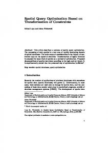
Where 𝑄 represents the set of all possible join orders, Σ represents all possible exchanges between two tables in the left deep join query three, 𝛿 is the transition function from one query plan to another with a symbol of Σ, 𝑞! , is a random element of 𝑄 selected as the initial state of the automaton, 𝐹, is the same set as 𝑄 because every plan in 𝑄 represents a solution, 𝑋! , is the vector that contains the order in 𝑞! and 𝑓(𝑋! ), is the objective function that estimates the cost of executing a given 𝑋! plan. The solution space that a DFAS can represent is reduced to all possible left deep trees and thus no bushy tree strategy can be directly explored by this method. To illustrate how to construct a DFAS modeling the join-ordering problem, Figure 1 shows the transition diagram of the DFAS corresponding to the following query with three tables to join. SELECT FROM WHERE
* tab1, tab2, tab3 tab1.fkt2 = tab2.pk AND tab2.fkt3 = tab3.pk
Figure 1. DFAS transition diagram from the example query
The transition diagram shows how the solution space of the join ordering problem is represented. Each node of the graph contains a vector with a join ordering in the left deep strategy of the following form: 𝑡1, 𝑡2, 𝑡3 → ((𝑡1 ⋈ 𝑡2) ⋈ 𝑡3)
(7)
Where the first two elements from left to right are joined first, and then the intermediate table is joined with the next element in the vector, creating another intermediate table. The process is repeated until there are no more elements to join and the last intermediate table contains the expected result. EDA was proposed as a method to navigate the DFAS structure without building the complete solution space, by the exploration of the neighborhood of a given state and an objective function improvement rule. Even though EDA is capable of finding global optimal solutions to combinatorial problems effectively, it was mainly designed to find optimal solutions to the traveling salesman problem. Despite the similarities between the TSP and the join-ordering problem, it is necessary to adjust the algorithm to perform as well in the solution of the query optimization problem, which is the targeted problem of this work. The main reason EDA is not efficient in the solution of the join-ordering problem is that the objective function used in the optimization procedure is yet an estimate of the real cost of using a specific join order. Therefore, minimal improvements towards a better solution may not be worth the effort of a new iteration of the algorithm. Another important reason EDA is not effective when applied to the query optimization problem is the lack of representation of the wider solution space, which includes bushy query trees. A slower convergence of
the algorithm is caused because it encounters a reasonable number of solutions with Cartesian products in the optimization process of the left-deep only solution space. In order to improve the convergence speed of the query optimization based on automata theory module, the DSQO algorithm was designed. There were two main improvements made to the original EDA algorithm: an objective function improvement criterion was added in order to avoid unnecessary optimization efforts and a heuristic was included to transform Cartesian product left-deep plans into feasible bushy tree query plans. The heuristic used was taken from the genetic implementation in PostgreSQL. The objective function improvement criterion added to the algorithm is used to stop the optimization process when the significance of the new optimum found is not relevant in the solution of the problem. An input parameter 𝜏 ∈ [0,1], which can be seen as a threshold value, is required by DSQO to evaluate if the new solution found in the iteration improves the current solution by a certain percentage given by 𝜏 using the following equation.
𝜑 − 𝛾!