Spatial Query Optimization Based on

Spatial Query Optimization Based on Transformation of Constraints Michal Lupa and Adam Pi´orkowski

Abstract This article describes a problem of spatial query optimization. The processing of such queries is a new area of rapidly developing domain of spatial databases. The main scope of considerations is the impact of constraints type on the speed of execution. Transformation of logical formulas is proposed for some kind of queries as a method of optimization. Proposed decompositions of queries were done according to the logic and set theory. It is experimentally proved that the presented way of optimization is efficient1 . Key words: spatial databases, query optimization

1 Introduction Recently the number of applications of relational databases with extensions for spatial data (spatial databases) still grows [1]. Unfortunately, in most cases, these systems are used only as storage for spatial data, and the processing of these data mostly takes place in specialized programs, outside of database management systems (DBMS). The development of spatial data Michal Lupa Department of Geoinformatics and Applied Computer Science, AGH University of Science and Technology, al. Mickiewicza 30, 30-059 Cracow, Poland, e-mail: [email protected] Adam Piorkowski Department of Geoinformatics and Applied Computer Science, AGH University of Science and Technology, al. Mickiewicza 30, 30-059 Cracow, Poland, e-mail: [email protected] 1

This is the accepted version of:

Lupa M., Piorkowski, A.: Spatial Query Optimization Based on Transformation of Constraints. Man-Machine Interactions 3, AISC vol. 242, Springer, 2014, pp 621-629 The original publication is available on www.springerlink.com

1

2

M. Lupa and A. Piorkowski

analysis methods has resulted in the SQL language extensions, namely, the first standard by OGC [2, 3], adding basic operations on points and shapes, and then the second, which is a separate section of the standard SQL/MM (ISO) concerning spatial data (SQL/MM - Spatial) [4]. The increased interest in server-side spatial query processing should be expected. Predicting this trend the authors focus on query optimization problems associated with spatial data, because this subject is rarely discussed, while the query optimization in general is a well known issue. Among the articles related to the optimization of spatial queries is one of the first works [5], related to the algebraic transformation of queries. The analysis and proposals for optimizing joins based on spatial attributes is certainly a very interesting study [6]. In articles [7, 8, 9] authors considered the possibility of using the Peano algebra for decomposition of queries. There has been achieved a significant reduction in query execution times. Another approach that allows to shorten the time of query execution is a generalization of objects [10], which in the case of lossless generalization is fully justified and effective (if it is possible), in the case of lossy generalization - at a given quality indicator allows for significant acceleration of queries. The spatial joins are the scope of the article [11]. The authors consider two different strategies: window reduction and synchronous traversal, that take advantage of underlying spatial indexes to effectively prune the search space. They provide cost models and optimization methods that combine the two strategies to compute more efficient execution plans. Comparison of spatial indexing has been studied extensively in the literature [12]. The authors compared the effectiveness of commonly used methods of R-trees with respect to XBR-trees. A very interesting approach is presented in thesis [13]. The authors proposed an extension for spatial data as well as the spatial processing functions by multi-layer mechanism. The next part of this paper also includes consideration of a framework for increasing the efficiency of the optimal query plans. Increase of performance of the queries type Point-In-Polygon using GPUs (Graphics Processing Units) is presented in the article [14]. Another approach of GPU using in spatial query acceleration is described in [15]. Previous work of authors involves a proposal of three methods for decomposition of queries [16]. There are considered transformations of constraints. As a result three rules for query optimization are proposed. The methods included in this article are underpinned by mathematical proofs in comparison to the previous article [16], where their validity has been demonstrated only at experimental level. Moreover, query transformations were performed with the basis of De Morgan’s laws and properties of the algebra of sets that are not used in the approach of the previous article.

Spatial Query Optimization

3

2 Decomposition Of Spatial Queries Based On Logical Operators Spatial data contain information on the coordinates and type of geometrical objects according to the OGC specifications (Open GIS Consortium). Increase in the amount of data increases the server-side query processing time. Therefore, optimization of these queries is an important issue. Selecting queries, which are based on joins on two or more tables are very time consuming because they check the spatial relations between geometric objects, which takes more time than checking constraints based on simple types. Moreover, the use of nested geometric data in functions contained in the spatial DBMS extensions, results in the creation of additional objects in memory. The effect is a significant reduction in database performance, which is a bottle-neck of spatial query processing performance.

2.1 Decomposition of Disjoint Constraints One of the frequent operations is checking whether the objects are disjoint. Disjoint in the context of operations on geometric data can be defined as follows: ¬∃x(x ∈ A ∧ x ∈ B)

(1)

where A, B - layers with geometric objects. Available tool that enables you to analyze the interaction of geometric objects according to the above relation is a function of Disjoint, implemented according to standard OGC: Disjoint (g1 Geometry, g2 Geometry) : Integer The parameters are spatial objects: g1 and g2. As a result, the function returns the integer 1 (TRUE) if the intersection of g1 and g2 is an empty set and 0 (FALSE), if the objects overlap. An example problem is to test the disconnection of three layers, where the two of them form a logical sum. A query implementing the solution of this task includes condition that consists of a combination of Disjoint and U nion functions. It makes the processing time longer. A solution that increases database performance is the decomposition of complex SQL query using Boolean operators. The proposed optimization method is replacing the function of the logical U nion by suitably decomposed query, that is based on Boolean operator AND. Let A, B, C are geometric objects, defined in three different layers, respectively, g1, g2, g3 and A ∈ g1, B ∈ g2, C ∈ g3. In addition, a Disjoint function, according to the standard OGC takes the value TRUE, if A ∩ B = ∅. It can be written symbolically as ¬(A ∩ B). Therefore, the disjointness can be written as:

4

M. Lupa and A. Piorkowski

¬((A ∪ B) ∩ C) ⇐⇒ ¬(A ∩ C) ∩ ¬(B ∩ C)

(2)

The expression: ¬((A ∪ B) ∩ C)

(3)

can be rewritten using the distributive law with respect to disjunction of conjunction: ¬((A ∩ C) ∪ (B ∩ C)) (4) And then according to the second of De Morgan’s law (negation of a disjunction): ¬(A ∩ C) ∩ ¬(B ∩ C)

(5)

A diagram illustrating the above consideration is shown in Fig. 1, on the next diagrams there are illustrated operations on the sum of the layers (Fig. 2) and disjoint operations on the separate layers (Fig. 3). There is an

Fig. 1 A diagram that illustrates A, B and C layers

tundra, swamp, trees

sum of two layers(tundra and trees)

disjoint of sum of two layers

and swamp

(tundra and trees) and swamp

Fig. 2 A diagram that illustrates operations on the sum of the layers, corresponding to Fig. 1

analysis of three layers (”tundra”, ”trees” and ”swamp”) in the study. These layers are included in sample spatial data of the Alaska region, provided by

Spatial Query Optimization

5

Input layers: trees and swamp (L), disjoint of input layerers (R)

Input layers: tundra and swamp (L), disjoint of input layerers (R)

Fig. 3 A diagram that illustrates disjoint operations on the separate layers, corresponding to Fig. 1 TREES

FID SHAPE CAT VEGDESC F_CODEDESC F_CODE AREA

TUNDRA

FID SHAPE CAT F_CODEDESC F_CODE AREA

SWAMP

FID SHAPE CAT F_CODEDESC F_CODE AREA

Fig. 4 The Alaska database partial schema

QuantumGIS software, as schema presented in Fig. 4. The proposed questions are related to disjoint of areas covered by forest or tundra with a layer that represents a place where there are swamps. Tests were carried out in two variants: • Q1 - The first option is to take into account the sum of the logical layers ”tundra” and ”trees” formed the basis of the spatial feature U nion: SELECT COUNT(*)FROM tundra,trees,swamp WHERE DISJOINT ( UNION (tundra.the_geom, trees.the_geom), swamp.the_geom ); • Q2 - The second version of query Q1, decomposed by using the Boolean operator AND:

6

M. Lupa and A. Piorkowski

SELECT COUNT(*)FROM tundra,trees,swamp WHERE DISJOINT (tundra.the_geom,swamp.the_geom) AND DISJOINT (trees.the_geom,swamp.the_geom);

2.1.1 Testing environment Queries were tested on the server-class computer IBM Blade with Windows 7 32 bit operating system included two database management systems: PostgreSQL 9.0.4 with the spatial extension PostGIS 1.5.0 and Spatialite 3.0.0. MySQL Spatial does not implement the standard correctly [17]. Server hardware configuration is as follows: IBM Blade HS 21, CPU: 2.0 GHz Intel Xeon (8 cores), RAM 16 GB, HDD 7200 rpm. Because of the long duration of the individual queries the size of each table was reduced to 30 rows. The tests were conducted ten times, the results (minimal query times) are shown in Fig. 5.

50000 45000

44134 40924

min query time [ms]

40000 35000 30000 25000 20000 15000 10000 5000

1389

312 0 Q1

Q2 PostgreSQL

Q1

Q2 Spatialite

Fig. 5 Minimal Q1 and Q2 query execution times.

2.2 Decomposition of Difference Constraints The geoprocessing of spatial data (vector and raster) requires the user to construct queries, which structure is based on algebra of sets. As a result, dedicated solutions often implement the functions of relational algebra. These

Spatial Query Optimization

7

functions as well as the method for determining object disjointness are decrease efficiency, in the case of they are components of nested spatial query. One of these functions is difference, which can be defined as follows: The difference between set A and set B is the set A\B of all elements, which belong to set A and not belong to set B: (x ∈ X\Y ) ⇐⇒ (x ∈ X ∧ x ∈ / Y)

(6)

The OGC Standard [2,3] describes the implementation of difference as: Difference (g1 Geometry,g2 Geometry) : Geometry Arguments of the function are sets of geometric objects: g1 and g2. The result is returned as the objects, which belong to set g1 and not belong to set g2. Spatial analysis in the most cases rely on determination of the area of objects that match to the complex criteria. The shown problem involves the determination of the tundra region, with an area of more than 100 km2 and which does not coincidence with swamps and forests. The difference of three layers makes the solution of this task is time-consuming, because the nested query loop creates additional objects in memory. The proposed optimization method is based on the query transformations, which are the result of algebra of sets properties. The decomposed query includes the logical operator OR and replacement difference to intersection. The difference of three geometric objects can be written as follows: A\(B\C)

(7)

Then by replacing difference B\C to intersection B ∩C ′ (The Difference Law, where C ′ is the negation of the set C) the expression takes the form: A\(B ∩ C ′ )

(8)

Using De Morgan’s Law for sets we receive the sum of the difference of set A and B and the difference of set A and negation of set C: (A\B) ∪ (A\C ′ )

(9)

Next step is to replace difference A\C ′ to intersection, according to the previously adopted rules. (A\B) ∪ (A ∩ C) (10) As the research there are proposed two variants of equivalent queries Q3 and Q4, developed according to the proof presented above. The queries Q3 and Q4 are performed on the same dataset as Q1 and Q2: • Q3 - The third option illustrates the difference between ”tundra”, ”trees” and ”swamp”, developed by the nested query.

8

M. Lupa and A. Piorkowski

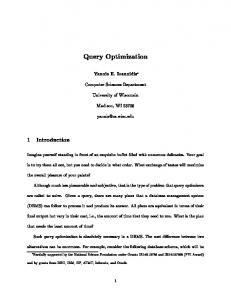
SELECT Count(*) FROM tundra, trees ,swamp WHERE ST_Area( ST_Difference( ST_Difference(tundra.the_geom, trees.the_geom), swamp.the_geom)) > 100; • Q4 - the option shows query Q3, which is decomposed using the presented transformations based on the algebra of sets rules. SELECT Count(*) FROM tundra ,trees, swamp WHERE ST_Area( ST_Difference(tundra.the_geom, swamp.the_geom)) > 100 OR ST_Area( ST_Intersection(trees.the_geom ,swamp.the_geom)) > 100; The tests were conducted ten times in the same hardware and software environment, the results (minimal query times) are shown in Fig. 6.

200000 181375 180000

min query time [ms]

160000

153500

140000 120000 99552 100000 80000

68594

60000 40000 20000 0 Q3

Q4 PostgreSQL

Q3

Q4 Spatialite

Fig. 6 Minimal Q3 and Q4 query execution times.

3 Conclusions The results of the first test indicate that the decomposed query using Boolean operator ”AND” performs over 131 times faster (40 924 ms and 312 ms Q1 to Q2) for the PostgreSQL DBMS with PostGIS and over 31 times faster for the SpatiaLite (44 134 ms for the Q1 and 1389 for the Q2), than those that use the ”UNION”. In case of Difference function decomposition, the speedups are

Spatial Query Optimization

9

lower, but still significant (223% for Q3 to Q4 for PostgreSQL+PostGIS and 182% for SpatiaLite). This confirms the validity of the proposed methods of optimization. Acknowledgements This work was financed by the AGH - University of Science and Technology, Faculty of Geology, Geophysics and Environmental Protection as a part of statutory project.

References 1. Krawczyk A, (2011). Attribute and Topology of Geometric Objects Systematics Attempt in Geographic Information Systems. Studia Informatica Vol. 32, No. 2B, 189– 201. 2. OGC - The Open Geospatial Consortium, http://www.opengeospatial.org/ 3. OpenGIS Implementation Specification for Geographic information - Simple feature access - SQL option. http://www.opengeospatial.org/standards/sfs 4. ISO/IEC 13249-3:1999, Information technology - Database languages - SQL Multimedia and Application Packages - Part 3: Spatial, International Organization For Standardization, 2000. 5. Helm R, Marriott K, Odersky M, (1991). Constraint-Based Query Optimization for Spatial Databases. Proc. 10th ACM PODS. 6. Park HH, Lee YJ, Chung CW, (2000). Spatial Query Optimization Utilizing Early Separated Filter and Refinement Strategy. Information Systems Vol. 25, No. 1, 1–22 7. Bajerski P, (2008). Optimization of geofield queries. Proceedings of the 1st International Conference on Information Technology, Gdansk, Poland. 8. Bajerski P, Kozielski S, (2009). Computational Model for Efficient Processing of Geofield Queries. International Conference on Man-Machine Interactions (ICMMI 2009), Advances in Intelligent and Soft Computing, Vol. 59, pp. 573–583 9. Bajerski P., (2009). How to Efficiently Generate PNR Representation of a Qualitative Geofield. Man-Machine Interactions Advances in Intelligent and Soft Computing Volume 59, pp. 595–603 10. Piorkowski A, Krawczyk A, (2011). The Problem of Object Generalization and Query Optimization in Spatial Databases. Studia Informatica Vol. 32, No. 2B, 119–129. 11. Papadias D, Mamoulis N, Theodoridis Y, (2001). Constraint-based processing of multiway spatial joins. ALGORITHMICA, Vol. 30, Iss. 2, Special Issue: SI, pp. 188–215 12. Roumelis G., Vassilakopoulos M., Corral A., (2011).Performance Comparison of xBRtrees and R*-trees for Single Dataset Spatial Queries. Advances in Databases and Information Systems, Lecture Notes in Computer Science, Vol. 6909, pp 228–242 13. Yan X., Chen R., Cheng C.,Peng X.,(2010). Spatial query processing engine in spatially enabled database. 18th International Conference on Geoinformatics, pp 1–6. 14. Zhang, J. and You., S. (2012). Speeding up Large-Scale Point-in-Polygon Test Based Spatial Join on GPUs. Technical report. 15. Aptekorz M, Szostek K, Mlynarczuk M, (2012). Spatial database acceleration using graphic card processors and user-defined functions. Studia Informatica Vol. 33, No. 2B, pp 145–152. 16. Lupa M, Piorkowski A, (2012). Rule-based Query Optimizations in Spatial Databases. Studia Informatica Vol. 33, No. 2B, 105–115. 17. Piorkowski A, (2011). Mysql Spatial and Postgis - Implementations Of Spatial Data Standards. EJPAU 14(1), no. 03.