Automata: from logics to algorithms∗ Moshe Y. Vardi1 Thomas Wilke2 1
Department of Computer Science Rice University 6199 S. Main Street Houston, TX 77005-1892, U.S.A.
[email protected] 2
Institut f¨ ur Informatik Christian-Albrechts-Universit¨ at zu Kiel Christian-Albrechts-Platz 4 24118 Kiel, Germany
[email protected]
Abstract We review, in a unified framework, translations from five different logics—monadic second-order logic of one and two successors (S1S and S2S), linear-time temporal logic (LTL), computation tree logic (CTL), and modal µ-calculus (MC)—into appropriate models of finite-state automata on infinite words or infinite trees. Together with emptiness-testing algorithms for these models of automata, this yields decision procedures for these logics. The translations are presented in a modular fashion and in a way such that optimal complexity bounds for satisfiability, conformance (model checking), and realizability are obtained for all logics.
1
Introduction
In his seminal 1962 paper [17], B¨ uchi states: “Our results [. . . ] may therefore be viewed as an application of the theory of finite automata to logic.” He was referring to the fact that he had proved the decidability of the monadic-second order theory of the natural numbers with successor function by translating formulas into finite automata, following earlier work by himself [16], Elgot [35], and Trakthenbrot [122]. Ever since, the approach these pioneers were following has been applied successfully in many different contexts and emerged as a major paradigm. It has not only brought about a number of decision procedures for mathematical theories, for instance, for the monadic second-order theory of the full binary tree [100], ∗
We are grateful to Detlef K¨ ahler, Christof L¨ oding, Oliver Matz, Damian Niwi´ nski, and Igor Walukiewicz for comments on drafts of this paper.
J¨ org Flum, Erich Gr¨ adel, Thomas Wilke (eds.). Logic and Automata: History and Perspectives. Texts in Logic and Games 2, Amsterdam University Press 2007, pp. 629–736.
630
M. Y. Vardi, Th. Wilke
but also efficient algorithms for problems in verification, such as a highly useful algorithm for LTL model checking [124]. The “automata-theoretic paradigm” has been extended and refined in various aspects over a period of more than 40 years. On the one hand, the paradigm has led to a wide spectrum of different models of automata, specifically tailored to match the distinctive features of the logics in question, on the other hand, it has become apparent that there are certain automatatheoretic constructions and notions, such as determinization of automata on infinite words [85], alternation [90], and games of infinite duration [12, 54], which form the core of the paradigm. The automata-theoretic paradigm is a common thread that goes through many of Wolfgang Thomas’s scientific works. In particular, he has written two influential survey papers on this topic [118, 120]. In this paper, we review translations from five fundamental logics, monadic second-order logic of one successor function (S1S), monadic secondorder logic of two successor functions (S2S), linear-time temporal logic (LTL), computation tree logic (CTL), and the modal µ-calculus (MC) into appropriate models of automata. At the same time, we use these translations to present some of the core constructions and notions in a unified framework. While adhering, more or less, to the chronological order as far as the logics are concerned, we provide modern translations from the logics into appropriate automata. We attach importance to present the translations in a modular fashion, making the individual steps as simple as possible. We also show how the classical results on S1S and S2S can be used to derive first decidability results for the three other logics, LTL, CTL, and MC, but the focus is on how more refined techniques can be used to obtain good complexity results. While this paper focuses on the translations from logics into automata, we refer the reader to the excellent surveys [118, 120] and the books [52, 96] for the larger picture of automata and logics on infinite objects and the connection with games of infinite duration. Basic notation and terminology Numbers. In this paper, the set of natural numbers is denoted ω, and each natural number stands for the set of its predecessors, that is, n = {0, . . . , n − 1}. Words. An alphabet is a nonempty finite set, a word over an alphabet A is a function n → A where n ∈ ω for a finite word and n = ω for an infinite word. When u : n → A is a word, then n is called its length and denoted |u|, and, for every i < n, the value u(i) is the letter of u in position i. The set of all finite words over a given alphabet A is denoted A∗ , the set of all infinite words over A is denoted Aω , the empty word is denoted ε, and A+
Automata: from logics to algorithms
631
stands for A∗ \ {ε}. When u is a word of length n and i, j ∈ ω are such that 0 ≤ i, j < n, then u[i, j] = u(i) . . . u(j), more precisely, u[i, j] is the word u0 of length max{j − i + 1, 0} defined by u0 (k) = u(i + k) for all k < |u0 |. In the same fashion, we use the notation u[i, j). When u denotes a finite, nonempty word, then we write u(∗) for the last letter of u, that is, when |u| = n, then u(∗) = u(n − 1). Similarly, when u is finite or infinite and i < |u|, then u[i, ∗) denotes the suffix of u starting at position i. Trees. In this paper, we deal with trees in various contexts, and depending on these contexts we use different types of trees and model them in one way or another. All trees we use are directed trees, but we distinguish between trees with unordered successors and n-ary trees with named successors. A tree with unordered siblings is, as usual, a tuple T = (V, E) where V is a nonempty set of vertices and E ⊆ V × V is the set of edges satisfying the usual properties. The root is denoted root(T ), the set of successors of a vertex v is denoted sucsT (v), and the set of leaves is denoted lvs(T ). Let n be a positive natural number. An n-ary tree is a tuple T = (V, suc0 , . . . , sucn−1 ) where V is the set of vertices and, for every i < n, suci is the ith successor relation satisfying the condition that for every vertex there is at most one ith successor (and the other obvious conditions). Every n-ary tree is isomorphic to a tree where V is a prefix-closed nonempty subset of n∗ and suci (v, v 0 ) holds for v, v 0 ∈ V iff v 0 = vi. When a tree is given in this way, simply by its set of vertices, we say that the tree is given in implicit form. The full binary tree, denoted Tbin , is 2∗ and the full ω-tree is ω ∗ . In some cases, we replace n in the above by an arbitrary set and speak of D-branching trees. Again, D-branching trees can be in implicit form, which means they are simply a prefix-closed subset of D∗ . A branch of a tree is a maximal path, that is, a path which starts at the root and ends in a leaf or is infinite. If an n-ary tree is given in implicit form, a branch is often denoted by its last vertex if it is finite or by the corresponding infinite word over n if it is infinite. Given a tree T and a vertex v of it, the subtree rooted at v is denoted T ↓v. In our context, trees often have vertex labels and in some rare cases edge labels too. When L is a set of labels, then an L-labeled tree is a tree with a function l added which assigns to each vertex its label. More precisely, for trees with unordered successors, an L-labeled tree is of the form (V, E, l) where l : V → E; an L-labeled n-ary tree is a tuple (V, suc0 , . . . , sucn−1 , l) where l : V → E; an L-labeled n-ary tree in implicit form is a function t : V → L where V ⊆ n∗ is the set of vertices of the tree; an L-labeled D-branching tree in implicit form is a function t : V → L where V ⊆ D∗ is the set of vertices of the tree. Occasionally, we also have more than one
632
M. Y. Vardi, Th. Wilke
vertex labeling or edge labelings, which are added as other components to the tuple. When T is an L-labeled tree and u is a path or branch of T , then the labeling of u in T , denoted lT (u), is the word w over L of the length of u and defined by w(i) = l(u(i)) for all i < |u|. Tuple Notation. Trees, graphs, automata and the like are typically described as tuples and denoted by calligraphic letters such as T , G , and so on, possibly furnished with indices or primed. The individual compo0 nents are referred to by V T , E G , E T , . . . . The ith component of a tuple t = (c0 , . . . , cr−1 ) is denoted pri (t).
2
Monadic second-order logic of one successor
Early results on the close connection between logic and automata, such as the B¨ uchi–Elgot–Trakhtenbrot Theorem [16, 35, 122] and B¨ uchi’s Theorem [17], center around monadic second-order logic with one successor relation (S1S) and its weak variant (WS1S). The formulas of these logics are built from atomic formulas of the form suc(x, y) for first-order variables x and y and x ∈ X for a first-order variable x and a set variable (monadic secondorder variable) X using boolean connectives, first-order quantification (∃x), and second-order quantification for sets (∃X). The two logics differ in the semantics of the set quantifiers: In WS1S quantifiers only range over finite sets rather than arbitrary sets. S1S and WS1S can be used in different ways. First, one can think of them as logics to specify properties of the natural numbers. The formulas are interpreted in the structure with the natural numbers as universe and where suc is interpreted as the natural successor relation. The most important question raised in this context is: Validity. Is the (weak) monadic second-order theory of the natural numbers with successor relation decidable? (Is a given sentence valid in the natural numbers with successor relation?) A slightly more general question is: Satisfiability. Is it decidable whether a given (W)S1S formula is satisfiable in the natural numbers? This is more general in the sense that a positive answer for closed formulas only already implies a positive answer to the first question. Therefore, we only consider satisfiability in the following. Second, one can think of S1S and WS1S as logics to specify the behavior of devices which get, at any moment in time, a fixed number of bits as input and produce a fixed number of bits as output (such as sequential circuits), see Figure 1. Then the formulas are interpreted in the same structure as above, but for every input bit and for every output bit there will be exactly
Automata: from logics to algorithms
2 32 32 3 0 0 1 607 607 617 ···4 54 54 5 1 1 1 0 0 0
633
2 32 32 3 0 1 0 . . . 405 415 415 1 0 0
sequential device
Figure 1. Sequential device one free set variable representing the moments in time where the respective bit is true. (The domain of time is assumed discrete; it is identified with the natural numbers.) A formula will then be true for certain input-output pairs—coded as variable assignments—and false for the others. For instance, when we want to specify that for a given device with one input bit, represented by the set variable X, and one output bit, represented by Y , it is the case that for every other moment in time where the input bit is true the output bit is true in the subsequent moment in time, we can use the following formula: ∃Z(“Z contains every other position where X is true” ∧ ∀x(x ∈ Z → “the successor of x belongs to Y ”)). That the successor of x belongs to Y is expressed by ∀y(suc(x, y) → y ∈ Y ). That Z contains every other position where X is true is expressed by the conjunction of the three following conditions, where we assume, for the moment, that the “less than” relation on the natural numbers is available: • Z is a subset of X, which can be stated as ∀x(x ∈ Z → x ∈ X), • If X is nonempty, then the smallest element of X does not belong to Z,
which can be stated as ∀x(x ∈ X ∧ ∀y(y < x → ¬y ∈ X) → ¬x ∈ Z). • For all x, y ∈ X such that x < y and such that there is no element of
X in between, either x or y belongs to Z, which can be stated as ∀x∀y(x ∈ X ∧ y ∈ X ∧ x < y ∧ ∀z(x < z ∧ z < y → ¬z ∈ X) → (x ∈ Z ↔ ¬y ∈ Z)). To conclude the example, we need a formula that specifies that x is less than y. To this end, we express that y belongs to a set which does not contain x but with each element its successor: ∃X(¬x ∈ X ∧ ∀z∀z 0 (z ∈ X ∧ suc(z, z 0 ) → z 0 ∈ X) ∧ y ∈ X).
634
M. Y. Vardi, Th. Wilke
The most important questions that are raised with regard to this usage of (W)S1S are: Conformance. Is it decidable whether the input-output relation of a given device satisfies a given formula? Realizability. Is it decidable whether for a given formula there exists a device with an input-output relation satisfying the formula (and if so, can a description of such a device be produced effectively)? Obviously, it is important what is understood by “device”. For instance, Church, when he defined realizability in 1957 [23], was interested in boolean circuits. We interpret device as “finite-state device”, which, on a certain level of abstraction, is the same as a boolean circuit. In this section, we first describe B¨ uchi’s Theorem (Section 2.1), from which we can conclude that the first two questions, satisfiability and conformance, have a positive answer. The proof of B¨ uchi’s Theorem is not very difficult except for a result about complementing a certain type of automaton model for infinite words, which we then establish (Section 2.2). After that we prove a result about determinization of the same type of automaton model (Section 2.3), which serves as the basis for showing that realizability is decidable, too. The other ingredient of this proof, certain games of infinite duration, are then presented, and finally the proof itself is given (Section 2.4). 2.1 B¨ uchi’s Theorem The connection of S1S and WS1S to automata theory, more precisely, to the theory of formal languages, is established via a simple observation. Assume that ϕ is a formula such that all free variables are set variables among V0 , . . . , Vm−1 , which we henceforth denote by ϕ = ϕ(V0 , . . . , Vm−1 ). Then the infinite words over [2]m , the set of all column vectors of height m with entries from {0, 1}, correspond in a one-to-one fashion to the variable assignments α : {V0 , . . . , Vm−1 } → 2ω , where 2M stands for the power set of any set M . More precisely, for every infinite word u ∈ [2]ω m let αu be the variable assignment defined by αu (Vj ) = {i < ω : u(i)[j] = 1}, where, for every a ∈ [2]m , the expression a[j] denotes entry j of a. Then αu ranges over all variable assignments as u ranges over all words in [2]ω m . As a consequence, we use u |= ϕ, or, when “weak quantification” (only finite sets are considered) is used, u |=w ϕ rather than traditional notation such as N, α |= ϕ (where N stands for the structure of the natural numbers). Further, when ϕ is a formula as above, we define two formal languages of infinite words depending on the type of quantification used: L (ϕ) = {u ∈ [2]ω m : u |= ϕ},
w L w (ϕ) = {u ∈ [2]ω m : u |= ϕ}.
Automata: from logics to algorithms
» – » – 0 0 , 0 1
635
» – » – » – 0 1 1 , , 0 1 » – » – 0 1 1 , 0 1
qI
» – 1 1
q1 » – 0 1
q2 » – 1 1
The initial state has an incoming edge without origin; final states are shown as double circles.
Figure 2. Example for a B¨ uchi automaton We say that ϕ defines the language L (ϕ) and weakly defines the language L w (ϕ). Note that, for simplicity, the parameter m is not referred to in our notation. B¨ uchi’s Theorem states that the above languages can be recognized by an appropriate generalization of finite-state automata to infinite words, which we introduce next. A B¨ uchi automaton is a tuple A = (A, Q, QI , ∆, F ) where A is an alphabet, Q is a finite set of states, QI ⊆ Q is a set of initial states, ∆ ⊆ Q × A × Q is a set of transitions of A , also called its transition relation, and F ⊆ Q is a set of final states of A . An infinite word u ∈ Aω is accepted by A if there exists an infinite word r ∈ Qω such that r(0) ∈ QI , (r(i), u(i), r(i + 1)) ∈ ∆ for every i, and r(i) ∈ F for infinitely many i. Such a word r is called an accepting run of A on u. The language recognized by A , denoted L (A ), is the set of all words accepted by A . For instance, the automaton in Figure 2 recognizes the language corresponding to the formula ∀x(x ∈ V0 → ∃y(x < y ∧ y ∈ V1 )), which says that every element from V0 is eventually followed by an element from V1 . In Figure 2, qI is the state where the automaton is not waiting for anything; q1 is the state where the automaton is waiting for an element from V1 to show up; q2 is used when from some point onwards all positions belong to V0 and V1 . Nondeterminism is used to guess that this is the case.
636
M. Y. Vardi, Th. Wilke
B¨ uchi’s Theorem can formally be stated as follows. Theorem 2.1 (B¨ uchi, [17]). 1. There exists an effective procedure that given a formula ϕ = ϕ(V0 , . . . , Vm−1 ) outputs a B¨ uchi automaton A such that L (A ) = L (ϕ) 2. There exists an effective procedure that given a B¨ uchi automaton A over an alphabet [2]m outputs a formula ϕ = ϕ(V0 , . . . , Vm−1 ) such that L (ϕ) = L (A ). The proof of part 2 is straightforward. The formula which needs to be constructed simply states that there exists an accepting run of A on the word determined by the assignment to the variables Vi . One way to construct ϕ is to write it as ∃X0 . . . ∃Xn−1 ψ where each set variable Xi corresponds exactly to one state of A and where ψ is a first-order formula (using < in addition to suc) which states that the Xi ’s encode an accepting run of the automaton (the Xi ’s must form a partition of ω and the above requirements for an accepting run must be satisfied): 0 must belong to one of the sets Xi representing the initial states; there must be infinitely many positions belonging to sets representing final states; the states assumed at adjacent positions must be consistent with the transition relation. The proof of part 1 is more involved, although the proof strategy is simple. The desired automaton A is constructed inductively, following the structure of the given formula. First-order variables, which need to be dealt with in between, are viewed as singletons. The induction base is straightforward and two of the three cases to distinguish in the inductive step are so, too: disjunction on the formula side corresponds to union on the automaton side and existential quantification corresponds to projection. For negation, however, one needs to show that the class of languages recognized by B¨ uchi automata is closed under complementation. This is not as simple as with finite state automata, especially since deterministic B¨ uchi automata are strictly weaker than nondeterministic ones, which means complementation cannot be done along the lines known from finite words. In the next subsection, we describe a concrete complementation construction. B¨ uchi’s Theorem has several implications, which all draw on the following almost obvious fact. Emptiness for B¨ uchi automata is decidable. This is easy to see because a B¨ uchi automaton accepts a word if and only if in its transition graph there is a path from an initial state to a strongly connected component which contains a final state. (This shows that emptiness can even be checked in linear time and in nondeterministic logarithmic space.)
Automata: from logics to algorithms
637
Given that emptiness is decidable for B¨ uchi automata, we can state that the first question has a positive answer: Corollary 2.2 (B¨ uchi, [17]). Satisfiability is decidable for S1S. Proof. To check whether a given S1S formula ϕ = ϕ(V0 , . . . , Vm−1 ) is satisfiable one simply constructs the B¨ uchi automaton which is guaranteed to exist by B¨ uchi’s Theorem and checks this automaton for non-emptiness. q.e.d. Observe that in the above corollary we use the term “satisfiability” to denote the decision problem (Given a formula, is it satisfiable?) rather than the question from the beginning of this section (Is it decidable whether . . . ). For convenience, we do so in the future too: When we use one of the terms satisfiability, conformance, or realizability, we refer to the corresponding decision problem. For conformance, we first need to specify formally what is meant by a finite-state device, or, how we want to specify the input-output relation of a finite-state device. Remember that we think of a device as getting inputs from [2]m and producing outputs from [2]n for given natural numbers m and n. So it is possible to view an input-output relation as a set of infinite words over [2]m+n . To describe an entire input-output relation of a finitestate device we simply use a nondeterministic finite-state automaton. Such an automaton is a tuple D = (A, S, SI , ∆) where A is an alphabet, S is a finite set of states, SI ⊆ S is a set of initial states, and ∆ ⊆ S × A × S is a transition relation, just as with B¨ uchi automata. A word u ∈ Aω is accepted by D if there exists r ∈ S ω with r(0) ∈ SI and (r(i), u(i), r(i + 1)) ∈ ∆ for every i < ω. The set of words accepted by D, denoted L (D), is the language recognized by D. Observe that L (D) is exactly the same as the language recognized by the B¨ uchi automaton which is obtained from D by adding the set S as the set of final states. Conformance can now be defined as follows: Given an S1S formula ϕ = ϕ(X0 , . . . , Xm−1 , Y0 , . . . , Yn−1 ) and a finite-state automaton D with alphabet [2]m+n , determine whether u |= ϕ for all u ∈ L (D). There is a simple approach to decide conformance. We construct a B¨ uchi automaton that accepts all words u ∈ L (D) which do not satisfy the given specification ϕ, which means we construct a B¨ uchi automaton which recognizes L (D) ∩ L (¬ϕ), and check this automaton for emptiness. Since B¨ uchi’s Theorem tells us how to construct an automaton A that recognizes L (¬ϕ), we only need a construction which, given a finite-state automaton D and a B¨ uchi automaton A , recognizes L (A ) ∩ L (D). The construction
638
M. Y. Vardi, Th. Wilke
The product of a B¨ uchi automaton A and a finite-state automaton D, both over the same alphabet A, is the B¨ uchi automaton denoted A × D and defined by A × D = (A, Q × S, QI × SI , ∆, F × S) where ∆ = {((q, s), a, (q 0 , s0 )) : (q, a, q 0 ) ∈ ∆A and (s, a, s0 ) ∈ ∆D }.
Figure 3. Product of a B¨ uchi automaton with a finite-state automaton depicted in Figure 3, which achieves this, is a simple automata-theoretic product. Its correctness can be seen easily. Since we already know that emptiness is decidable for B¨ uchi automata, we obtain: Corollary 2.3 (B¨ uchi, [17]). Conformance is decidable for S1S. From results by Stockmeyer and Meyer [112, 111], it follows that the complexity of the two problems from Corollaries 2.2 and 2.3 is nonelementary, see also [102]. Another immediate consequence of B¨ uchi’s Theorem and the proof of part 2 as sketched above is a normal form theorem for S1S formulas. Given an arbitrary S1S formula, one uses part 1 of B¨ uchi’s Theorem to turn it into an equivalent B¨ uchi automaton and then part 2 to reconvert it to a formula. The proof of part 2 of B¨ uchi’s Theorem is designed in such a way that a formula will emerge which is of the form ∃V0 . . . ∃Vn−1 ψ where ψ is without second-order quantification but uses 0 such that S , u(j) |= χ and S , u(i) |= ψ for all i with 0 < i < j.
• S , s |= A(ψ XU χ) if for all computations u of S starting at s there
exists j > 0 such that S , u(j) |= χ and S , u(i) |= ψ for all i with 0 < i < j.
Just as with LTL, other operators can be defined: • “in all computations always” is defined by AGϕ = ϕ ∧ ¬E(tt XU ¬ϕ), • “in some computation eventually” is defined by EFϕ = ϕ ∨ E(tt XU ϕ).
Automata: from logics to algorithms
697
An interesting property one can express in CTL is the one discussed above, namely that from every state reachable from a given state a distinguished state, indicated by the propositional variable pd , can be reached: AG EFpd .
(1.3)
Another property that can be expressed is that every request, indicated by the propositional variable pr , is eventually acknowledged, indicated by the propositional variable pa : AG(pr → AX AFpa ).
(1.4)
It is interesting to compare the expressive power of CTL with that of LTL. To this end, it is reasonable to restrict the considerations to infinite computations only and to say that a CTL formula ϕ and an LTL formula ψ are equivalent if for every transition system S and every state s ∈ S the following holds: S , s |= ϕ iff l(u(0))l(u(1)) . . . |= ψ for all infinite computations u of S starting in s. The second property from above can be expressed easily in LTL, namely by the formula G(pr → XFpa ), that is, this formula and (1.4) are equivalent. Clarke and Draghicescu showed that a CTL property is equivalent to some LTL formula if and only if it is equivalent to the LTL formula obtained by removing the path quantifiers [26]. But it is not true that every LTL formula which can be expressed in CTL is expressible by a CTL formula which uses universal path quantifiers only. This was shown by Bojanczyk [10]. An LTL formula which is not expressible in CTL is GFp,
(1.5)
which was already pointed out by Lamport [77]. In order to be able to recast satisfiability and model checking in a (tree) automata setting, it is crucial to observe that CTL formulas cannot distinguish between a transition system and the transition system obtained by “unraveling” it. Formally, the unraveling of the transition system S at state s ∈ S, denoted Ts (S ), is the tree inductively defined by: • s is the root of Ts (S ), • if v ∈ S + is an element of V Ts (S ) and v(∗) → s0 , then vs0 ∈ V Ts (S )
and (v, vs0 ) ∈ E Ts (S ) ,
• lTs (S ) (v) = lS (v(∗)) for every v ∈ V Ts (S ) .
Henceforth, a tree with labels from 2P , such as the unraveling of a transition system, is viewed as a transition system in the canonical way. When we
698
M. Y. Vardi, Th. Wilke
interpret a CTL formula in a tree and do not indicate a vertex, then the formula is interpreted at the root of the tree. The formal statement of the above observation can now be phrased as follows. Lemma 5.1. For every CTL formula ϕ, transition system S , and state s ∈ S, S , s |= ϕ
iff
Ts (S ) |= ϕ.
Proof. This can be proved by a straightforward induction on the structure of ϕ, using a slightly more general claim: S , s0 |= ϕ
iff
Ts (S ), v |= ϕ
for every state s0 ∈ S and every vertex v of Ts (S ) where v(∗) = s0 . q.e.d. The previous lemma says that we can restrict attention to trees, in particular, a CTL formula is satisfiable if and only if there is a tree which is a model of it. So when we translate CTL formulas into logics on trees which satisfiability is decidable for, then we also know that CTL satisfiability is decidable. We present a simple translation of CTL into monadic second-order logic. There is, however, an issue to be dealt with: S2S formulas specify properties of binary trees, but CTL is interpreted in transition systems where each state can have more than just two successors. A simple solution is to use a variant of S2S which allows any number of successors but has only a single successor predicate, suc. Let us denote the resulting logic by SUS. As with LTL, we identify the elements of 2P for P = {p0 , . . . , pn−1 } with the elements of [2]n . Proposition 5.2. Let P = {p0 , . . . , pn−1 } be an arbitrary finite set of propositional variables. For every CTL formula ϕ over P an SUS formula ϕ˜ = ϕ(X ˜ 0 , . . . , Xn−1 ) can be constructed such that T |= ϕ if and only if T |= ϕ˜ for all trees T over 2P (or [2]n ). Proof. What we actually prove is somewhat stronger, analogous to the proof for LTL. We construct a formula ϕˆ = ϕ(X ˆ 0 , . . . , Xn−1 , x) such that T , v |= ϕ if and only if T , v |= ϕˆ for all trees T and v ∈ V T . We can then set ϕ˜ = ∃x(ϕroot (x) ∧ ϕ) ˆ where ϕroot (x) = ∀y(¬suc(y, x)) specifies that x is the root. For the induction base, assume ϕ = pi . We can set ϕˆ to x ∈ Xi . Similarly, for ϕ = ¬pi we can set ϕˆ to ¬x ∈ Xi . In the inductive step, we consider only one of the interesting cases, namely where ϕ = A(ψ XU χ). We start with a formula ϕclosed = ϕclosed (X)
Automata: from logics to algorithms
699
which is true if every element of X has a successor in X provided it has a successor at all: ϕclosed = ∀x(x ∈ X ∧ ∃y(suc(x, y)) → ∃y(suc(x, y) ∧ y ∈ X)). We next write a formula ϕpath (x, X) which is true if X is a maximum path starting in x: ϕpath = x ∈ X ∧ ϕclosed (X) ∧ ∀Y (x ∈ Y ∧ ϕclosed (Y ) ∧ Y ⊆ X → X = Y ). We can then set ϕˆ = ∀X(ϕpath (x, X) → ˆ ∃z(z ∈ X ∧ ¬z = x ∧ χ(z) ˆ ∧ ∀y(x < y < z → ψ(y))). The other CTL operators can be dealt with in a similar fashion.
q.e.d.
The desired decidability result now follows from the following result on SUS. Theorem 5.3 (Walukiewicz, [128]). SUS satisfiability is decidable. This result can be proved just as we proved the decidability of satisfiability for S2S, that is, using an analogue of Rabin’s Theorem. This analogue will use a different kind of tree automaton model which takes into account that the branching degree of the trees considered is unbounded and that there is one predicate for all successors. More precisely, a transition in such an automaton is of the form (q, a, QE , QA ) where QE , QA ⊆ Q. Such a transition is to be read as follows: If the automaton is in state q at a vertex labeled a, then for every q 0 ∈ QE there exists exactly one successor that gets assigned q 0 and all the successors that do not get assigned any state in this fashion get assigned exactly one state from QA . In particular, if QE = QA = ∅, then the vertex must not have a successor. In [128], Walukiewicz actually presents a theorem like B¨ uchi’s and Rabin’s: He shows that there is a translation in both directions, from SUS formulas to such automata and back. Corollary 5.4. CTL satisfiability and model checking are decidable. That model checking is decidable follows from the simple observation that in SUS one can define the unraveling of every finite transition system. We conclude this introduction to CTL with further remarks on SUS and its relationship to CTL. There is a logic related to SUS which was already studied by Rabin and which he denoted SωS. This is the logic interpreted
700
M. Y. Vardi, Th. Wilke
in the countably branching tree ω ∗ where, for each i, there is a separate successor relation suci (·, ·). Observe that—as noted in [60]—in this logic one cannot even express that all successors of the root belong to a certain set, which can easily be expressed in CTL and SUS. Observe, too, that in SUS one can express that every vertex of a tree has at least two successors, namely by ∀x(∃y0 ∃y1 (suc(x, y0 ) ∧ suc(x, y1 ) ∧ ¬y0 = y1 ). This is, however, impossible in CTL. More precisely, CTL cannot distinguish between bisimilar transition systems whereas SUS can do this easily. 5.2 From CTL to nondeterministic tree automata We next show how to arrive at good complexity bounds for satisfiability and model checking by following a refined automata-theoretic approach. For satisfiability, we can use nondeterministic automata and vary the approach we used for handling LTL in Section 4, while for model checking, we have to use alternating tree automata. As pointed out above, the nondeterministic tree automaton model we defined in Section 3 was suited for binary trees only, which is not enough in the context of CTL. Here, we need an automaton model that can handle trees with arbitrary branching degree. We could use the tree automaton model explained in Section 5.1, but there is another model which is more appropriate. Following Janin and Walukiewicz [59], we use a tree automaton model which takes into account that properties like the one mentioned at the end of Section 5.1 cannot be expressed in CTL. A generalized B¨ uchi tree automaton in this context is a tuple A = (A, Q, QI , ∆, F ) where A, Q, QI , and F are as with generalized B¨ uchi (word) automata and ∆ ⊆ Q × A × 2Q × 2Q is a transition relation. A transition of the form (q, a, QE , QA ) is to be read as follows: If the automaton is in state q at vertex v and reads the label a, then it sends each state from QE to at least one of the successors of v and every successor of v is at least sent one of the states from QE ∪ QA ; the same successor can get sent several states. Formally, a run of A on a tree T is a (Q×V T )-labeled tree R satisfying the following conditions. (i) The root of R is labeled (q, root(T )) for some q ∈ QI . (ii) For every vertex w ∈ V R , if (q, v) is the label of w, then there exists a transition (q, lR (v), QE , QA ) ∈ ∆ such that:
Automata: from logics to algorithms
701
(a) For every v 0 ∈ sucsT (v) there exists w0 ∈ sucsR (w) labeled (q 0 , v 0 ) for some q 0 ∈ QE ∪ QA , that is, every successor of v occurs in a label of a successor of w. (b) For every q 0 ∈ QE there exist v 0 ∈ sucsT (v) and w0 ∈ sucsR (w) such that w0 is labeled (q 0 , v). That is, every state from QE occurs at least once among all successors of w. Such a run is accepting if every branch is accepting with respect to the given generalized B¨ uchi condition just as this was defined for generalized B¨ uchi word automata. Observe that in this model the unlabeled tree underlying a run may not be the same as the unlabeled tree underlying a given input tree. Copies of subtrees may occur repeatedly. As an example, let P = {p} and A = 2P and consider the tree language L which contains all trees over A that satisfy the property that every branch is either finite or labeled {p} infinitely often. An appropriate B¨ uchi automaton has two states, q∅ and q{p} , where q∅ is initial and q{p} is final, and the transitions are (q, a, {qa }) and (q, a, ∅, ∅) for any state q and letter a. The idea for translating a given CTL formula into a nondeterministic tree automaton follows the translation of LTL into nondeterministic word automata: In each vertex, the automaton guesses which subformulas of the given formula are true and verifies this. The only difference is that the path quantifiers E and A are taken into account, which is technically somewhat involved. The details are given in Figure 23, where the following notation and terminology is used. Given a set Ψ of CTL formulas over a finite set P of propositional variables and a letter a ∈ 2P we say that Ψ is consistent with a if • ff ∈ / Ψ, • p ∈ Ψ iff p ∈ a, for all p ∈ P , and • for ψ ∈ Ψ, if ψ = ψ0 ∨ ψ1 , then ψi ∈ Ψ for some i < 2, and if
ψ = ψ0 ∧ ψ1 , then {ψ0 , ψ1 } ⊆ Ψ. Further, a set Ψ0 is a witness for E(ψ XUχ) if χ ∈ Ψ0 or {ψ, E(ψ XUχ)} ⊆ Ψ0 . Similarly, Ψ0 is a witness for E(ψXRχ) if {ψ, χ} ⊆ Ψ0 or {χ, E(ψXRχ)} ⊆ Ψ0 . The analogue terminology is used for A-formulas. When Ψ is a set of CTL formulas, then ΨE denotes the formulas of the form E(ψXUχ) and E(ψXRχ), that is, the set of all E-formulas in Ψ, and, similarly, ΨA denotes the set of all A-formulas in Ψ. The only interesting aspect of the construction is (iv) of the definition of a transition. It would be more natural to omit (iv), and, indeed, the construction would then also be correct, but the resulting automaton would
702
M. Y. Vardi, Th. Wilke
Let P be a finite set of propositional variables and ϕ a CTL formula over P in positive normal form. The generalized B¨ uchi tree automaton for ϕ with respect to P , denoted A [ϕ], is defined by A [ϕ] = (2P , 2sub(ϕ) , QI , ∆, F ) where QI = {Ψ ⊆ 2sub(ϕ) : ϕ ∈ Ψ} and F = {FQ[ψXUχ] : Q[ψ XU χ] ∈ sub(ϕ) and Q ∈ {E, A}} with FQ[ψXUχ] = {Ψ ⊆ sub(ϕ) : χ ∈ Ψ or Q[ψ XU χ] ∈ / Ψ}, and where ∆ contains a transition (Ψ, a, QE , QA ) if the following conditions are satisfied: (i) Ψ is consistent with a, (ii) for every ψ ∈ ΨE there exists Ψ0 ∈ QE which witnesses it and QA contains all Ψ ⊆ sub(ϕ) that contain a witness for every ψ ∈ ΨA , (iii) every Ψ0 ∈ QE witnesses every ψ ∈ ΨA , (iv) QE ≤ |sub(ϕ)E |.
Figure 23. From CTL to generalized B¨ uchi tree automata be too large. On the other hand, (iv) is not a real restriction, because the semantics of CTL requires only one “witness” for every existential path formula. Before formally stating the correctness of the construction, we introduce a notion referring to the number of different states which can be assigned in a transition. We say that a nondeterministic tree automaton A is mbounded if QE ≤ m holds for every (q, a, QE , QA ) ∈ ∆. Lemma 5.5. Let ϕ be an arbitrary CTL formula with n subformulas, m E-subformulas, and k U-subformulas. Then A [ϕ] is an (m + 1)-bounded generalized B¨ uchi tree automaton with 2n states, k acceptance sets, and
Automata: from logics to algorithms
703
Let A be a nondeterministic B¨ uchi tree automaton. The emptiness game for A , denoted G∅ [A ], is defined by G∅ [A ] = (Q, ∆, qI , M0 ∪ M1 , F ) where M0 = {(q, QE , QA ) : ∃a∃QA ((q, a, QE , QA ) ∈ ∆)}, and M1 = {(Q0 , q) : q ∈ Q0 }.
Figure 24. Emptiness game for nondeterministic B¨ uchi tree automaton such that L (A [ϕ]) = L (ϕ). Proof sketch. The claim about the size of the automaton is trivial. The proof of its correctness can be carried out similar to the proof of Theorem 4.4, that is, one proves L (A [ϕ]) ⊆ L (ϕ) by induction on the structure of ϕ and L (ϕ) ⊆ L (A [ϕ]) by constructing an accepting run directly. q.e.d. It is very easy to see that the construction from Figure 18 can also be used in this context to convert a generalized B¨ uchi tree automaton into a B¨ uchi automaton. To be more precise, an m-bounded generalized B¨ uchi tree automaton with n states and k acceptance sets can be converted into an equivalent m-bounded B¨ uchi tree automaton with (k + 1)n states. So in order to solve the satisfiability problem for CTL we only need to solve the emptiness problem for B¨ uchi tree automata in this context. There is a simple way to perform an emptiness test for nondeterministic tree automata, namely by using the same approach as for nondeterministic tree automata working on binary trees: The nonemptiness problem is phrased as a game. Given a nondeterministic B¨ uchi tree automaton A , we define a game which Player 0 wins if and only if some tree is accepted by A . To this end, Player 0 tries to suggest suitable transitions while Player 1 tries to argue that Player 0’s choices are not correct. The details of the construction are given in Figure 24. Lemma 5.6. Let A be a nondeterministic B¨ uchi tree automaton. Then the following are equivalent: (A) L (A ) 6= ∅.
704
M. Y. Vardi, Th. Wilke
(B) Player 0 wins G∅ [A ]. Proof. The proof of the lemma can be carried out along the lines of the proof of Lemma 3.3. The only difference is due to the arbitrary branching degree, which can easily be taken care of. One only needs to observe that if there exists a tree which is accepted by A , then there is a tree with branching degree at most |Q| which is accepted. q.e.d. We have the following theorem: Theorem 5.7 (Emerson-Halpern-Fischer-Ladner, [37, 45]). CTL satisfiability is complete for deterministic exponential time. Proof. The decision procedure is as follows. A given CTL formula ϕ is first converted into an equivalent generalized B¨ uchi tree automaton A using the construction from Figure 23. Then A is converted into an equivalent B¨ uchi tree automaton B using the natural adaptation of the construction presented in Figure 18 to trees. In the third step, B is converted into the B¨ uchi game G∅ [B], and, finally, the winner of this game is determined. (Recall that a B¨ uchi condition is a parity condition with two different priorities.) From Theorem 2.21 on the complexity of parity games it follows immediately that B¨ uchi games (parity games with two different priorities) can be solved in polynomial time, which means we only need to show that the size of G∅ [B] is exponential in the size of the given formula ϕ and can be constructed in exponential time. The latter essentially amounts to showing that B is of exponential size. Let n be the number of subformulas of ϕ. Then A is n-bounded with 2n states and at most n acceptance sets. This means that the number 2 of sets Q0 occurring in the transitions of A is at most 2n , so there are 2 at most 2n +2n transitions (recall that there are at most 2n letters in the alphabet). Similarly, B is n-bounded, has at most (n + 1)2n states, and 2 2O(n ) transitions. The lower bound is given in [45]. q.e.d. 5.3 From CTL to alternating tree automata One of the crucial results of Emerson and Clarke on CTL is that model checking of CTL can be carried out in polynomial time. The decision procedure they suggested in [28] is a simple labeling algorithms. For every subformula ψ of a given formula ϕ they determine in which states of a given transition system S the formula ψ holds and in which it does not hold. This is trivial for atomic formulas. It is straightforward for conjunction and disjunction, provided it is known which of the conjuncts and disjuncts, respectively, hold. For XR- and XU-formulas, it amounts to simple graph searches.
Automata: from logics to algorithms
705
Emerson and Clarke’s procedure cannot easily be seen as a technique which could also be derived following an automata-theoretic approach. Consider the nondeterministic tree automaton we constructed in Figure 23. Its size is exponential in the size of the given formula (and this cannot be avoided), so it is unclear how using this automaton one can arrive at a polynomial-time procedure. The key for developing an automata-theoretic approach, which is due to Kupferman, Vardi, and Wolper [71], is to use alternating tree automata similar to how we used alternating automata for LTL in Section 4 and to carefully analyze their structure. An alternating B¨ uchi tree automaton is a tuple A = (P, Q, qI , δ, F ) where P , Q, qI , and F are as usual and δ is the transition function which assigns to each state a transition condition. The set of transition conditions over P and Q, denoted TC(P, Q), is the smallest set such that (i) tt, ff ∈ TC(P, Q), (ii) p, ¬p ∈ TC(P, Q) for every p ∈ P , (iii) every positive boolean combination of states is in TC(P, Q), (iv) 3γ, 2γ ∈ TC(P, Q) where γ is a positive boolean combination of states. This definition is very similar to the definition for alternating automata on words. The main difference reflects that in a tree a “position” can have several successors: 3 expresses that a copy of the automaton should be sent to one successor, while 2 expresses that a copy of the automaton should be sent to all successors. So 3 and 2 are the two variants of #. There is another, minor difference: For tree automata, we allow positive boolean combinations of states in the scope of 3 and 2. We could have allowed this for word automata, too, but it would not have helped us. Here, it makes our constructions simpler, but the proofs will be slightly more involved. Let T be a 2P -labeled tree. A tree R with labels from TC(P, Q) × T V is a run of A on T if lR (root(R)) = (qI , root(T )) and the following conditions are satisfied for every vertex w ∈ V R with label (γ, v): • γ 6= ff, • if γ = p, then p ∈ lT (w), and if γ = ¬p, then p ∈ / lT (w),
706
M. Y. Vardi, Th. Wilke
• if γ = 3γ 0 , then there exists v 0 ∈ sucsT (v) and w0 ∈ sucsR (w) such
that lR (w0 ) = (γ 0 , v 0 ),
• if γ = 2γ 0 , then for every v 0 ∈ sucsT (v) there exists w0 ∈ sucsR (w)
such that lR (w0 ) = (γ 0 , v 0 ),
• if γ = γ0 ∨ γ1 , then there exists i < 2 and w0 ∈ sucsR (w) such that
lR (w0 ) = (γi , v),
• if γ = γ0 ∧ γ1 , then for every i < 2 there exists w0 ∈ sucsR (w) such
that lR (w0 ) = (γi , v).
Such a run is accepting if on every infinite branch there exist infinitely many vertices w labeled with an element of F in the first component. The example language from above can be recognized by an alternating B¨ uchi automaton which is slightly more complicated than the nondeterministic automaton, because of the restrictive syntax for transition conditions. 0 We use the same states as above and four further states, q, q{p} , q⊥ , and 0 q⊥ . The transition function is determined by δ(qI ) = q⊥ ∨ q, 0 δ(q{p} ) = q{p} ∧ (q⊥ ∨ q), 0 δ(q⊥ ) = 2q⊥ , δ(q) = 2(qI ∨ q{p} ).
0 δ(q{p} ) = p, 0 δ(q⊥ ) = ff,
The state q⊥ is used to check that the automaton is at a vertex without successor. In analogy to the construction for LTL, we can now construct an alternating tree automaton for a given CTL formula. This construction is depicted in Figure 25. Compared to the construction for LTL, there are the following minor differences. First, the definition of the transition function is no longer inductive, because we allow positive boolean combinations in the transition function. Second, we have positive boolean combinations of states in the scope of 3 and 2. This was not necessary with LTL, but it is necessary here. For instance, if we instead had δ([E(ψXUχ)]) = 3[χ]∨(3[ψ]∧3[E(ψXUχ)]), then this would clearly result in a false automaton because of the second disjunct. We can make a similar observation as with the alternating automata that we constructed for LTL formulas. The automata are very weak in the sense that when we turn the subformula ordering into a linear ordering ≤ on the states, then for each state q, the transition conditions δ(q) contains only states q 0 such that q ≥ q 0 .
Automata: from logics to algorithms
707
Let ϕ be a CTL formula in positive normal form over P and Q the set which contains for each ψ ∈ sub(ϕ) an element denoted [ψ]. The automaton A alt [ϕ] is defined by A alt [ϕ] = (P, Q, [ϕ], δ, F ) where δ([tt]) = tt, δ([p]) = p, δ([ψ ∨ χ]) = [ϕ] ∨ [ψ],
δ([ff]) = ff, δ([¬p]) = ¬p, δ([ψ ∧ χ]) = [ϕ] ∧ [ψ],
δ([E(ψ XU χ)]) = 3([χ] ∨ ([ψ] ∧ [E(ψ XU χ)])), δ([E(ψ XR χ)]) = 3([χ] ∧ ([χ] ∨ [E(ψ XR χ)])),
δ([A(ψ XU χ)]) = 2([χ] ∨ ([ψ] ∧ [A(ψ XU χ)])), δ([A(ψ XR χ)]) = 2([χ] ∧ ([χ] ∨ [A(ψ XR χ)])),
and F contains all the elements [ψ] where ψ is not an XUformula.
Figure 25. From CTL to alternating tree automata Lemma 5.8 (Kupferman-Vardi-Wolper, [71]). Let ϕ be a CTL formula with n subformulas. The automaton A alt [ϕ] is a very weak alternating tree automaton with n states and such that L (A alt [A]) = L (ϕ). Proof. The proof can follow the lines of the proof of Lemma 4.7. Since the automaton is very weak, a simple induction on the structure of the formula can be carried out, just as in the proof of Lemma 4.7. Branching makes the proof only technically more involved, no new ideas are necessary to carry it out. q.e.d. As pointed out above, it is not our goal to turn A alt [ϕ] into a nondeterministic automaton (although this is possible), because such a translation cannot be useful for solving the model checking problem. What we rather do is to define a product of an alternating automaton with a transition system, resulting in a game, in such a way that the winner of the product of A alt [ϕ] with some transition system S reflects whether ϕ holds true in a certain state sI of S .
708
M. Y. Vardi, Th. Wilke
The idea is that a position in this game is of the form (γ, s) where γ is a transition condition and s is a state of the transition system. The goal is to design the game in such a way that Player 0 wins the game starting from (qI , sI ) if and only if there exists an accepting run of the automaton on the unraveling of the transition system starting at sI . This means, for instance, that if γ is a disjunction, then we make the position (γ, s) a position for Player 0, because by moving to one of the two successor positions he should show which of the disjuncts holds. If, on the other hand, γ = 2γ 0 , then we make the position a position for Player 1, because she should be able to challenge Player 0 with any successor of s. The details are spelled out in Figure 26, where the following notation and terminology is used. Given an alternating automaton A , we write sub(A ) for the set of subformulas of the values of the transition function of A . In addition, we write sub+ (A ) for the set of all γ ∈ sub(A ) where the maximum state occurring belongs to the set of final states. Assume A is a very weak alternating B¨ uchi automaton. Then A ×sI S is not very weak in general in the sense that the game graph can be extended to a linear ordering. Observe, however, that the following is true for every position (q, s): All states in the strongly connected component of (q, s) are of the form (γ, s0 ) where q is the largest state occurring in γ. So, by definition of A ×sI S , all positions in a strongly connected component of A ×sI S are either final or nonfinal. We turn this into a definition. We say that a B¨ uchi game is weak if for every strongly connected component of the game graph it is true that either all its positions are final or none of them is. Lemma 5.9. Let A be an alternating B¨ uchi tree automaton, S a transition system over the same finite set of propositional variables, and sI ∈ S. Then TsI (S ) ∈ L (A ) iff Player 0 wins A ×sI S . Moreover, if A is a very weak alternating automaton, then A ×sI S is a weak game. Proof. The additional claim is obvious. For the other claim, first assume R is an accepting run of A on TsI (S ). We convert R into a winning strategy σ for Player 0 in A ×S . To this end, let w be a vertex of R with label (γ, v) such that (γ, v) is a position for Player 0. Since R is an accepting run, w has a successor, say w0 . Assume lR (w0 ) = (γ 0 , v 0 ). We set σ(u) = (γ, v 0 (∗)) where u is defined as follows. First, let n = |v|. Assume lR (u(i)) = (γi , vi ) for every i < n. We set u = (γ0 , v0 (∗))(γ1 , v1 (∗)) . . . (γn−1 , vn−1 (∗)). It can be shown that this defines a strategy. Moreover, since R is accepting, σ is winning. For the other direction, a winning strategy is turned into an accepting run in a similar manner. q.e.d. The proof shows that essentially there is no difference between a run and a strategy—one can think of a run as a strategy. From this point of
Automata: from logics to algorithms
709
Let A be an alternating B¨ uchi tree automaton, S a transition system over the same set of propositional variables, and sI ∈ S. The product of A and S at sI , denoted A ×sI S , is the B¨ uchi game defined by A ×sI S = (P0 , P1 , (qI , sI ), M, sub+ (A ) × S) where • P0 is the set of pairs (γ, s) ∈ sub(A ) × S where γ is
(i) a disjunction, (ii) a 3-formula,
(iii) p for p ∈ / l(s), (iv) ¬p for p ∈ l(s), or (v) ff, and • P1 is the set of pairs (γ, s) ∈ sub(A ) × S where γ is
(i) a conjunction, (ii) a 2-formula,
(iii) p for some p ∈ l(s), (iv) ¬p for some p ∈ / l(s), or (v) tt. Further, M contains for every γ ∈ sub(A ) and every s ∈ S moves according to the following rules: • if γ = q for some state q, then ((γ, s), (δ(q), s)) ∈ M , • if γ = γ0 ∨ γ1 or γ = γ0 ∧ γ1 , then ((γ, s), (γi , s)) ∈ M
for i < 2, • if γ = 3γ 0 or γ = 2γ 0 , then ((γ, s), (γ 0 , s0 )) ∈ M for all
s0 ∈ sucsS (s).
Figure 26. Product of a transition system and an alternating automaton
710
M. Y. Vardi, Th. Wilke
view, an alternating automaton defines a family of games, for each tree a separate game, and the tree language recognized by the tree automaton is the set of all trees which Player 0 wins the game for. The additional claim in the above lemma allows us to prove the desired complexity bound for the CTL model checking problem: Theorem 5.10 (Clarke-Emerson-Sistla, [28]). The CTL model checking problem can be solved in time O(mn) where m is the size of the transition system and n the number of subformulas of the CTL formula. Proof. Consider the following algorithm, given a CTL formula ϕ, a transition system S , and a state sI ∈ S. First, construct the very weak alternating B¨ uchi automaton A alt [ϕ]. Second, build the product A alt [ϕ] ×sI S . Third, solve A alt [ϕ] ×sI S . Then Player 0 is the winner if and only if S , sI |= ϕ. The claim about the complexity follows from the fact that the size of A alt [ϕ]×sI S is mn and from Theorem 2.21. Note that weak games are parity games with one priority in each strongly connected component. q.e.d. Obviously, given a CTL formula ϕ, a transition system S , and a state sI one can directly construct a game that reflects whether S , sI |= ϕ. This game would be called the model checking game for S , sI , and ϕ. The construction via the alternating automaton has the advantage that starting from this automaton one can solve both, model checking and satisfiability, the latter by using a translation from alternating B¨ uchi tree automata into nondeterministic tree automata. We present such a translation in Section 6. The translation from CTL into very weak alternating automata has another interesting feature. Just as the translation from LTL to weak alternating automata, it has a converse. More precisely, following the lines of the proof of Theorem 4.9, one can prove: Theorem 5.11. Every very weak alternating tree automaton is equivalent to a CTL formula. q.e.d. 5.4 Notes The two specification logics that we have dealt with, LTL and CTL, can easily be combined into a single specification logic. This led Emerson and Halpern to introduce CTL∗ in 1986 [38]. An automata-theoretic proof of Corollary 5.7 was given first by Vardi and Wolper in 1986 [125]. Kupferman, Vardi, and Wolper, when proposing an automata-theoretic approach to CTL model checking in [71], also showed how other model checking problems can be solved following the automatatheoretic paradigm. One of their results is that CTL model checking can be solved in space polylogarithmic in the size of the transition system.
Automata: from logics to algorithms
6
711
Modal µ-calculus
The logics that have been discussed thus far—S1S, S2S, LTL, and CTL— could be termed declarative in the sense that they are used to describe properties of sequences, trees, or transition systems rather than to specify how it can be determined whether such properties hold. This is different for the logic we discuss in this section, the modal µ-calculus (MC), introduced by Kozen in 1983 [66]. This calculus has a rich and deep mathematical and algorithmic theory, which has been developed over more than 20 years. Fundamental work on it has been carried out by Emerson, Streett, and Jutla [114, 40], Walukiewicz [129], Bradfield and Lenzi [79, 11], and others, and it has been treated extensively in books, for instance, by Arnold and Niwi´ nski [6] and Stirling [110]. In this section, we study satisfiability (and model checking) for MC from an automata-theoretic perspective. Given that MC is much more complex than LTL or CTL, our exposition is less detailed, but gives a good impression of how the automata-theoretic paradigm works for MC. 6.1 MC and monadic second-order logic MC is a formal language consisting of expressions which are evaluated in transition systems; every closed expression (without free variables) is evaluated to a set of states. The operations available for composing sets of states are boolean operations, local operations, and fixed point operations. Formally, the set of MC expressions is the smallest set containing • p and ¬p for any propositional variable p, • any fixed-point variable X, • ϕ ∧ ψ and ϕ ∨ ψ if ϕ and ψ are MC expressions, • h iϕ and [ ]ϕ if ϕ is an MC expression, and • µXϕ and νXϕ if X is a fixed-point variable and ϕ an MC expression.
The operators µ and ν are viewed as quantifiers in the sense that one says they bind the following variable. As usual, an expression without free occurrences of variables is called closed. The set of all variables occurring free in an MC expression ϕ is denoted by free(ϕ). An expression is called a fixed-point expression if it starts with µ or ν. To define the semantics of MC expressions, let ϕ be an MC expression over some finite set P of propositional variables, S a transition system, and α a variable assignment which assigns to every fixed-point variable a set of states of S . The value of ϕ with respect to S and α, denoted ||ϕ||α S,
712
M. Y. Vardi, Th. Wilke
is defined as follows. The fixed-point variables and the propositional variables are interpreted according to the variable assignment and the transition system: S S ||p||α S = {s ∈ S : p ∈ l (s)},
S ||¬p||α / lS (s)}, S = {s ∈ S : p ∈
and ||X||α S = α(X). Conjunction and disjunction are translated into union and intersection: α α ||ϕ ∧ ψ||α S = ||ϕ||S ∩ ||ψ||S ,
α α ||ϕ ∨ ψ||α S = ||ϕ||S ∪ ||ψ||S .
The two local operators, h i and [ ], are translated into graph-theoretic operations: S α ||h iϕ||α S = {s ∈ S : sucs (s) ∩ ||ϕ||S 6= ∅}, S α ||[ ]ϕ||α S = {s ∈ S : sucs (s) ⊆ ||ϕ||S }.
The semantics of the fixed-point operators is based on the observation that α[X7→S 0 ] for every expression ϕ, the function S 0 7→ ||ϕ||S is a monotone function on 2S with set inclusion as ordering, where α[X 7→ S 0 ] denotes the variable assignment which coincides with α, except for the value of the variable X, which is S 0 . The Knaster–Tarski Theorem then guarantees that this function has a least and a greatest fixed point: o \n α[X7→S 0 ] 0 0 ||µXϕ||α = S ⊆ S : ||ϕ|| = S , S S o [n 0 α[X7→S ] ||νXϕ||α S 0 ⊆ S : ||ϕ||S = S0 . S = In the first equation the last equality sign can be replaced by ⊆, while in the second equation it can be replaced by ⊇. The above equations are—contrary to what was said at the beginning of this section—declarative rather than operational, but this can easily be changed because of the Knaster–Tarski Theorem. For a given system S , a variable assignment α, an MC expression ϕ, and a fixed-point variable X, consider the ordinal sequence (Sλ )λ , called approximation sequence for ||µXϕ||α S , defined by [ α[X7→Sλ ] S0 = ∅, Sλ+1 = ||ϕ||S , Sλ0 = Sλ , λ νX1 ψ1 > µX2 ψ2 > · · · > µ/νXl−1 ψl−1
(1.6)
where, for every i < l − 1, the variable Xi occurs free in every formula ψ with ψi ≥ ψ ≥ ψi+1 . The maximum length of an alternating µ-chain in ϕ is denoted by mµ (ϕ). Symmetrically, ν-chains and mν (ϕ) are defined. The alternation depth of a µ-calculus expression ϕ is the maximum of mµ (ϕ) and mν (ϕ) and is denoted by d(ϕ). We say an MC expression is in normal form if for every fixed-point variable X occurring the following holds: • every occurrence of X in ϕ is free or • all occurrences of X in ϕ are bound in the same subexpression µXψ
or νXψ, which is then denoted by ϕX . Clearly, every MC expression is equivalent to an MC expression in normal form. The full translation from MC into alternating parity tree automata can be found in Figure 27, where the following notation is used. When ϕ is an MC expression and µXψ ∈ sub(ϕ), then ( d(ϕ) + 1 − 2dd(µXψ)/2e, if d(ϕ) mod 2 = 0, dϕ (µXψ) = d(ϕ) − 2bd(µXψ)/2c, otherwise. Similarly, when νXψ ∈ sub(ϕ), then ( d(ϕ) − 2bd(νXψ)/2c, if d(ϕ) mod 2 = 0, dϕ (νXψ) = d(ϕ) + 1 − 2dd(νXψ)/2e, otherwise. This definition reverses alternation depth so it can be used for defining the priorities in the alternating parity automaton for an MC expression. Recall that we want to assign priorities such that the higher the alternation depth the lower the priority and, at the same time, even priorities go to ν-formulas
Automata: from logics to algorithms
717
Let ϕ be a closed MC expression in normal form and Q a set which contains for every ψ ∈ sub(ϕ) a state [ψ]. The alternating parity tree automaton for ϕ, denoted A [ϕ], is defined by A [ϕ] = (P, Q, ϕ, δ, π) where the transition function is given by δ([¬p]) = ¬p,
δ([p]) = p, δ([ψ ∨ χ]) = [ψ] ∨ [χ], δ([h iψ]) = 3[ψ], δ([µXψ]) = [ψ], δ([X]) = [ϕX ],
δ([ψ ∧ χ]) = [ψ] ∧ [χ], δ([[ ]ψ]) = 2[ψ], δ([νXψ]) = [ψ],
and where π([ψ]) = dϕ (ψ) for every fixed-point expression ψ ∈ sub(ϕ).
Figure 27. From µ-calculus to alternating tree automata and odd priorities to µ-formulas. This is exactly what the above definition achieves. It is obvious that A [ϕ] will have d(ϕ) + 1 different priorities in general, but from a complexity point of view, these cases are not harmful. To explain this, we introduce the notion of index of an alternating tree automaton. The transition graph of an alternating tree automaton A is the graph with vertex set Q and where (q, q 0 ) is an edge if q 0 occurs in δ(q). The index of A is the maximum number of different priorities in the strongly connected components of the transition graph of A . Clearly, A [ϕ] has index d(ϕ). Theorem 6.5 (Emerson-Jutla, [40]). Let ϕ be an MC expression in normal form with n subformulas. Then A [ϕ] is an alternating parity tree automaton with n states and index d(ϕ) such that L (A [ϕ]) = L (ϕ). To be more precise, A [ϕ] may have d(ϕ) + 1 different priorities, but in every strongly connected component of the transition graph of A [ϕ] there are at most d(ϕ) different priorities, see also Theorem 2.21.
718
M. Y. Vardi, Th. Wilke
Proof. The claims about the number of states and the index are obviously true. The proof of correctness is more involved than the corresponding proofs for LTL and CTL, because the automata which result from the translation are, in general, not weak. The proof of the claim is by induction on the structure of ϕ. The base case is trivial and so are the cases in the inductive step except for the cases where fixed-point operators are involved. We consider the case where ϕ = µXψ. So assume ϕ = µXψ and T |= ϕ. Let f : 2V → 2V be defined by X7→V 0 .SLet (Vλ )λ be the sequence defined by V0 = ∅, Vλ+1 = f (V 0 ) = ||ψ||T f (Vλ ), and Vλ0 = λ