including the trace that skips the loop entirely, and traces containing the loop body ..... recursive programs typically compile to assembler programs for which no ...... is a way to ignore such other causes of infeasibility, causes unrelated to the.
Automated Control Flow Reconstruction from Assembler Programs Dominik Klumpp
Masterarbeit im Elitestudiengang Software Engineering
Institut für Software & Systems Engineering Universitätsstraÿe 6a
D-86135 Augsburg
WEBSTYLEGUIDE
Automated Control Flow Reconstruction from Assembler Programs Matrikelnummer:
1321113
Beginn der Arbeit:
12. Juni 2018
Abgabe der Arbeit:
12. Dezember 2018
Erstgutachter:
Prof. Dr. Wolfgang Reif
Zweitgutachter:
Prof. Dr. Bernhard Bauer
Betreuer:
Prof. Dr. Franck Cassez Dr. Gerhard Schellhorn
Institut für Software & Systems Engineering Universitätsstraÿe 6a
D-86135 Augsburg
WEBSTYLEGUIDE
4
Erklärung Hiermit versichere ich, dass ich diese Masterarbeit selbständig verfasst habe. Ich habe dazu keine anderen als die angegebenen Quellen und Hilfsmittel verwendet.
Augsburg, den 10. Dezember 2018
Dominik Klumpp
5
6
Abstract As software permeates more and more aspects of daily life and becomes a central component of critical systems around the world, software quality and e�ective methods to ensure it are paramount. There is a huge variety of both static and dynamic analyses that aim to provide such guarantees. Typically, such analyses are based on the analysed program's control �ow graph (CFG). Given the source code of the program in a high-level, structured programming language, this graph can easily be constructed. However, in some cases the analysis must instead be based directly on the binary program, e.g. if the source code is not available (in security contexts), contains insu�cient information (e.g. for low-level analyses such as execution time) or the compiler is not trusted to translate the source code faithfully to a binary format. However, extracting the control �ow graph from a binary program is a non-trivial task, as the binary code is unstructured and contains indirect branches that transfer control to a program location dynamically computed at runtime. This thesis de�nes a formal notion of a CFG for a binary program and proposes several quality requirements such CFGs should meet in order to be considered a su�ciently precise approximation of the program. A more precise CFG improves the e�ciency and potentially the accuracy of subsequent analyses.
In particular, we de�ne the property of being free from control
�ow errors and postulate that precise CFGs should satisfy this property. The CFGs produced by existing approaches to control �ow reconstruction from binary programs do not meet all of these requirements. A new approach to control �ow reconstruction is thus presented, based on the formal veri�cation technique trace abstraction re�nement. This veri�cation technique is adapted to the �eld of control �ow reconstruction, and the computed CFGs are shown to be sound over-approximations of the program behaviour. A su�cient condition is presented under which the CFGs are furthermore free from control �ow errors. We evaluate the new approach empirically on a set of standard benchmark programs.
7
8
Acknowledgements This thesis would not have been possible without the support of many people. I wish to express my gratitude to all those who have helped me over the past few months. The research presented in this thesis was conducted in cooperation with and at Macquarie University, Sydney. My primary thanks goes to my Australian supervisor, Professor Franck Cassez, for the opportunity to come to Australia and to research this topic, for many long discussions about the nature of control �ow, the introduction to trace abstraction re�nement, and much more. Furthermore, I want to thank everyone at the programming languages and veri�cation research group, all the students in room E6D, and everyone at the Computing Department, for welcoming me and making my stay not only productive but also very enjoyable. I also want to thank my German supervisor at the University of Augsburg, Dr. Gerhard Schellhorn, for all his help and his constructive and immensely useful feedback on the presentation of this complex subject matter. I am very grateful to Professor Wolfgang Reif, who agreed to be the advisor and �rst examiner for my thesis, and, together with Dr. Dominik Haneberg and Professor Peter Höfner, helped me establish the contact with Macquarie University and Franck Cassez, thus enabling my stay there.
Furthermore,
I would like to thank Professor Bernhard Bauer, the second examiner of my thesis.
Special thanks also to Philip Lenzen for his proofreading and
feedback.
9
10
Contents 1 Introduction
13
2 Control Flow Reconstruction: Overview
15
2.1
A Minimal Example
. . . . . . . . . . . . . . . . . . . . . . .
15
2.2
Dealing with Loops . . . . . . . . . . . . . . . . . . . . . . . .
18
2.3
A Schematic Algorithm
20
. . . . . . . . . . . . . . . . . . . . .
3 Basic De�nitions
23
3.1
Instruction Sets . . . . . . . . . . . . . . . . . . . . . . . . . .
23
3.2
Programs
26
. . . . . . . . . . . . . . . . . . . . . . . . . . . . .
4 Capturing Control Flow
31
4.1
Properties of Control Flow Graphs
. . . . . . . . . . . . . . .
31
4.2
Possible Control Flow Graphs . . . . . . . . . . . . . . . . . .
36
5 Resolving Traces
39
5.1
Handling Simple Instructions
. . . . . . . . . . . . . . . . . .
40
5.2
SMT-Based Location Computation . . . . . . . . . . . . . . .
42
5.3
Craig Interpolation . . . . . . . . . . . . . . . . . . . . . . . .
44
5.4
Weakest Precondition
45
. . . . . . . . . . . . . . . . . . . . . .
6 A Control Flow Reconstruction Algorithm
47
6.1
Resolver Automata . . . . . . . . . . . . . . . . . . . . . . . .
47
6.2
The Reconstruction Algorithm
52
. . . . . . . . . . . . . . . . .
7 The Infeasibility Problem
57
7.1
Problem and Solution Approach . . . . . . . . . . . . . . . . .
58
7.2
Solution Heuristics
60
7.3
. . . . . . . . . . . . . . . . . . . . . . . .
7.2.1
Variable Interdependence Projection
. . . . . . . . . .
60
. . . . . . . . . . . . . .
62
Integration with Inductive Sequences . . . . . . . . . . . . . .
7.2.2
Further Heuristical Solutions
63
11
CONTENTS
8 Extensions to the Algorithm
67
8.1
Optimization for Simple Instructions . . . . . . . . . . . . . .
67
8.2
Concretizing Instructions
. . . . . . . . . . . . . . . . . . . .
69
8.3
Resolver Minimization
. . . . . . . . . . . . . . . . . . . . . .
76
9 Evaluation
77
9.1
Implementation . . . . . . . . . . . . . . . . . . . . . . . . . .
77
9.2
Results . . . . . . . . . . . . . . . . . . . . . . . . . . . . . . .
78
10 Conclusion
87
10.1 Summary of Results
. . . . . . . . . . . . . . . . . . . . . . .
87
10.2 Advantages and Limitations . . . . . . . . . . . . . . . . . . .
88
10.3 Related Work . . . . . . . . . . . . . . . . . . . . . . . . . . .
89
10.4 Future Work
91
. . . . . . . . . . . . . . . . . . . . . . . . . . .
A Selection of Generated CFGs
12
97
Chapter 1
Introduction Qualitative and quantitative analyses of software play a crucial role in assuring software quality: Veri�cation can prove program correctness, worst case execution time (WCET) analysis can be used to guarantee real-time properties, automated optimization for executable size or runtime can reduce storage space or response time, and security analyses can increase con�dence in untrusted code. Many of these analyses are based on the control �ow graph of the analysed software. When the analysed program is given as source code in a typical high-level programming language, this is no problem as the control �ow graph can easily be derived. However, in some cases the analysis must be based on the compiled binary containing assembler code instead of the high-level source code. For instance, such an analysis is necessary if the source code is unavailable (especially in security contexts), does not contain enough low-level information (as in the WCET case), or the compiler is untrusted, i.e., unveri�ed. To apply standard analyses in this case, the control �ow graph must be extracted from the assembler code. This is not as easy as it is for source code written in highlevel programming languages, because the common control �ow constructs do not exist.
Instead, the program �ow is controlled through a so-called
program counter, or
pc,
which holds the memory address of the next atomic
piece of code (or instruction ) to be executed; and through jump or branch
instructions, which modify the program counter in non-trivial ways. The key problem in the construction of control �ow graphs for binary programs is the problem of indirect branches, which transfer control to a location dynamically computed during runtime. There are di�erent features of programming languages that typically produce such assembler code. Most commonly, the return from a procedure or function call must transfer control to the correct call site, which is determined during runtime, speci�cally at the time of the function or procedure call.
Other such language features
include switches, calls via function pointers, and exception handling. Due to the dynamic nature of such indirect jumps, control �ow analysis of binary 13
CHAPTER 1.
INTRODUCTION
programs is notoriously di�cult: The control �ow depends on the data �ow of the program, which in turn depends on the control �ow � they are inseparably intertwined. Existing research into control �ow reconstruction either lacks a precise formal speci�cation of the requirements for the reconstruction algorithm, or de�nes a single target graph which is then over-approximated. By contrast, this work will consider a very abstract and general notion of a control �ow graph for a program.
We will then state and formally de�ne several
requirements for control �ow graphs, and show how existing de�nitions do not satisfy all these requirements.
Namely, we propose that CFGs should
(1) over-approximate the program behaviour, but that the approximation should not be too imprecise, i.e., that the CFGs should (2) be free from
control �ow errors, a property that we de�ne and motivate formally.
We
argue that these requirements should be met by control �ow reconstruction approaches, and that they are bene�cial to subsequent formal analyses of the generated graph. Furthermore, we present a new approach to the construction of CFGs from assembler programs, based on trace abstraction re�nement [1, 2], a software veri�cation technique.
The approach is generic in the assembler
language, and relies only on few assumptions. In particular, it does not assume availability of any debugging information, nor on the well-formedness of the assembler code.
We prove that the CFGs constructed by this ap-
proach always over-approximate the program behaviour � our �rst quality requirement �, and under a su�cient condition we can also show that they approximate it precisely enough to be free from control �ow errors � our second quality requirement. While completeness does not hold, we show empirically that the approach is successful for many typical programs. We will focus entirely on the control �ow reconstruction part, leaving qualitative or quantitative analyses that can be performed on the reconstructed CFG as a separate step. The remainder of the thesis is structured as follows: Chapter 2 showcases the core principle of the reconstruction approach on two examples, and presents an overview of the individual components. After these intuitive descriptions, chapter 3 will give a number of foundational de�nitions, preparing the ground for chapter 4, which formalizes the notion of a CFG and the requirements for sensible CFGs. Chapter 5 describes a central component of our approach in detail, chapter 6 then de�nes the entire reconstruction approach formally.
In chapter 7, we investigate a key shortcoming of the
algorithm as presented so far, and discuss strategies to compensate for it. Further extensions to the algorithm are described in chapter 8. Finally, we present our implementation in chapter 9 along with some evaluation results. We conclude with an overview of our results and a discussion of related as well as future work in chapter 10.
14
Chapter 2
Control Flow Reconstruction: Overview This chapter gives an overview of our approach using two examples.
The
�rst example takes a high-level view and shows how our approach iteratively expands a fragment of the control �ow graph. The second example explains how trace abstraction re�nement techniques, including our approach, deal with an in�nite number of traces introduced by the existence of loops. The presentation in this chapter is inspired by the presentation of an approach to probabilistic veri�cation by Smith et al. [3], whereas the commonalities in content are restricted to the basic features of trace abstraction re�nement [1, 2], on which both approaches are based.
2.1
A Minimal Example
For our �rst example, let us consider the simple, loop-free program given in listing 2.1. It is written in ARM assembler code, which we will use for examples throughout the thesis. Our implementation, as seen in chapter 9, also implements control �ow reconstruction for this assembler language.
0000: bl 0004: bl 0008: b
0040 ; lr := 0004 , goto 0040 0040 ; lr := 0008 , goto 0040 0008 ; goto 0008 ( halt )
0040: bx
lr
; goto value of lr
Listing 2.1:
A program demonstrating two calls to a function.
The program is a condensed version of a program calling a function (lo-
0040) twice, from two di�erent call sites, at location 0000 0004; a commonly occurring control �ow pattern. In assembler, the function calls are encoded as bl instructions, setting a special link return
cated at address and location
15
CHAPTER 2.
CONTROL FLOW RECONSTRUCTION: OVERVIEW
0000: bl 0040
τp1 : true
true
0040: bx lr true
lr
0004: bl 0040 true
Figure 2.1:
register
pc “ 0004
lr “ 0004
0000: bl 0040
τp2 :
t 0004 u
0040: bx lr
0040: bx lr
t 0008 u
pc “ 0008
lr “ 0008
Traces of the program in listing 2.1.
to the address of the subsequent instruction before transferring
control to the given address,
0040 in this case.
The function is a trivial one,
it returns directly to the caller. In order to return to the correct call site, it uses the link return register via the instruction
bx lr.
lr
and transfers control to the stored address
This instruction is an indirect branch, it transfers
control to the dynamically computed value stored in its argument register. We will iteratively construct fragments of the control �ow graph for this program, beginning with the initial program location (in our examples, this will always be location
0000).
The instruction at this location is
The next program location after executing this instruction will be
bl 0040. 0040, as
is clearly visible from the instruction itself, without considering any context. However, the next step is more complex: Looking only at the instruction at
0040, bx lr,
we cannot predict the next location, as it depends on
the unknown value of
Instead we need to consider it in its context, i.e.,
location
lr.
the preceding sequence of instructions (or trace ) executed by the program. In this case, the relevant trace
τp1
is given in �g. 2.1.
To this point, we have constructed the CFG fragment seen in �g. 2.2a. For the expansion of this fragment we require the possible program locations after execution of
τp1 .
In order to compute these locations for a given trace,
we transform it into static single assignment-form (SSA) and encode it as a logical formula.
The encoding of
τp1
and a second trace,
τp2
in �g. 2.1, are
given below:
"
* lr1 “ pc1 ` 4 pc ^ loooomoooon pc3 “ lr1 1 “ 0000 ^ looooomooooon pc2 “ 0040 looooooooooomooooooooooon
initial location
0000: bl 0040
(2.1)
0040: bx lr
"
* lr1 “ pc1 ` 4 pc ^ loooomoooon pc3 “ lr1 1 “ 0000 ^ looooomooooon pc2 “ 0040 looooooooooomooooooooooon
initial location
0000: bl 0040
0040: bx lr
"
* lr2 “ pc3 ` 4 ^ ^ pc 5 “ lr2 loooomoooon pc4 “ 0040 looooooooooomooooooooooon 0004: bx lr 16
0040: bx lr
(2.2)
2.1.
A MINIMAL EXAMPLE
bl 0040
0000
(a)
bl 0040
?
bx lr
0040
0000
(b)
Expanded until the �rst indirect
bl 0040
0040
bx lr
0040
bl 0040
0004
Location of indirect branch is com-
puted, but CFG node is unclear.
branch is encountered.
bl 0040 0000
bl 0040
0000
0040
bx lr
bx lr
0040
0004
bl 0040
0004
b 0008
bx lr
(c)
bl 0040
0040
0008
Selecting the existing node for
0040
(d)
bx lr
0008
The �nal, precise CFG.
yields an imprecise CFG.
Figure 2.2:
Iterative construction of the CFG for listing 2.1.
Examining the encoding of must be
0004
τp1 ,
eq. (2.1), we conclude the value of
pc3
in all models of the formula, and therefore this is the only
possible program location after execution of this trace. In general, a trace can have multiple successor locations; or equivalently, the formula encoding of the trace can have models with di�ering values for the �nal our result takes the form of a set of locations, in �g. 2.1. Similarly, for
τp2
t 0004 u,
we �nd the set of locations
0004,
Therefore
t 0008 u.
Next, the control �ow analysis considers the instruction tion
pcn .
annotated in orange
bl 0040 at loca-
and concludes as before that the only successor location for such
an instruction can be location
0040.
However, in order to create more pre-
cise CFGs, our approach will sometimes create multiple nodes with the same location. Therefore it is at this point unclear whether we should reuse the existing CFG node labeled with location
0040, or create a new one (�g. 2.2b).
Let us assume for the moment that we reuse the existing node, as we have so far no reason to create a new one. This yields the CFG seen in �g. 2.2c. Our analysis of
τp2
has shown us that whatever node we chose, it must
have a successor node labeled
0008.
However, if we add this successor to the
chosen existing node, the created CFG (hinted at in �g. 2.2c) is imprecise: It includes traces that skip the second function call and return to location
0008
after the �rst call, as well as traces with an unlimited number of repetitions of the second function call. Neither of these re�ects the program's actual control �ow, hence we wish to exclude such traces. We therefore (retroactively) split the node labeled
0040
into two nodes, as we now have found a reason to
di�erentiate. After expanding the direct branch at location at the �nal, precise CFG in �g. 2.2d. 17
0008,
we arrive
CHAPTER 2.
2.2
CONTROL FLOW RECONSTRUCTION: OVERVIEW
Dealing with Loops
In the previous example, we were in the fortunate situation that whenever we encountered an indirect branch, there was only a single trace leading to it in the CFG. Hence we were able to compute the possible target locations in the context of this single trace and continue. However, in the general case, there may be more than one, or in the presence of loops, even an in�nite number of traces leading to a single indirect branch. This is where the power of trace abstraction re�nement comes into play: We analyse the branch in the context of a single trace, and soundly generalize the computed result to an in�nite number of traces, described by a regular language. The following program, listing 2.2, will illustrate this generalization. As before, we have a function call encoded as a body in this case contains a
do/while-style
bl
instruction. The function
loop: It decrements a register
r0 (location 0040), and compares its new value to the constant 0 (location 0044). Location 0048 contains a conditional branch: If r0 was not equal (ne) to 0 at the time of the last comparison, bne will transfer control to location 0040, restarting the loop. Otherwise, the loop condition is violated and control falls through to location 004c, where the function once again returns via an indirect branch bx lr. 0000: bl 0004: b
0040 0004
0040: 0044: 0048: 004 c:
r0 , r0 , #1 ; r0 := r0 - 1 r0 , #0 ; compare r0 , 0 0040 ; goto 0040 if r0 =/= 0 lr ; goto value of lr
sub cmp bne bx
Listing 2.2:
; lr := 0004 , goto 0040 ; goto 0004 ( halt )
A program demonstrating a call to a function containing a loop.
Most instructions in this program do not directly in�uence the control �ow.
Therefore the successor locations of most traces can be determined
statically, given only the last instruction and its location. The key problem is again the indirect branch
bx lr1 ,
but this time there is a large number of
traces leading to this branch (one for each iteration count of the loop). The analysis begins by examining the trace
τp3 ,
given in �g. 2.3 (at the
top). By encoding the trace as a formula and collecting solutions for the �nal
pc as before, it concludes that the next program location must be 0004.
This
will hold for all traces, no matter the number of loop iterations. In order to prove this fact, we compute an inductive sequence ; in essence a Hoare-style
1
Technically, the successor location of the conditional (direct) branch
bne 0040
also
depends on the context. However, in this example we explore both options (the branch being taken or not), in order to avoid a too precise analysis. chapter 8 for more information.
18
Refer to chapter 7 and
2.2.
0000: bl 0040 0040: sub r0, r0, #1 0044: cmp r0, #0 true
lr “ 0004
lr “ 0004
DEALING WITH LOOPS
0048: bne 0040
lr “ 0004
004c: bx lr pc “ 0004
lr “ 0004
0040: sub r0, r0, #1 0044: cmp r0, #0 0048: bne 0040 0000: bl 0040
Rτp3 : true
Figure 2.3:
pc “ 0004
lr “ 0004
Generalizing from a single trace
proof that for the trace
τp3
t 0004 u
004c: bx lr
τp3
to a regular language
LpRτx3 q.
there can be no other locations. The predicate
annotations corresponding to this proof can be seen in �g. 2.3 annotated in blue along the trace. From this inductive sequence we construct a �nite
2
automaton, a so-called resolver .
As states, we take the predicates of the
proof, the alphabet is given by the program instructions, and every transition must form a valid Hoare triple.
The �rst resp.
last predicate are used as
initial resp. accepting state, and the accepting state is labeled with the set of locations we computed. and the annotated proof.
Figure 2.3 shows the resolver
Rτp3
given by
τp3
For any trace accepted by such a resolver, the
sequence of states by which it is accepted forms again an inductive sequence, proving that the program location after executing this trace must be one of those labeling the accepting state. Thereby the analysis result for one trace is generalized to a whole regular language of traces. regular language
LpRτp3 q
In our example, this
covers all traces reaching location
004c
(regardless
of the number of iterations), and hence we have concluded the analysis for this indirect jump. In general, we may have to analyse several traces, or even an in�nite number � termination is not guaranteed. It depends on a suitable choice of the
τp3 pc.
predicates forming the inductive sequence: For instance, in could include a conjunct specifying the current value of
each predicate The sequence
would still be inductive, but the resolver would have more states and accept fewer traces, thus not allowing such a broad generalization as with the given annotations. However, in most assembler programs, the number of iterations in a loop does not alter possible targets for an indirect branch following the loop. We discuss di�erent strategies to compute suitable predicates in chapter 5 and mention some further heuristic improvements in chapter 7. With these strategies, a loop often completely preserves the computed predicate throughout the loop (as in our example), or at least restores it at the end of the loop, i.e., it forms a loop invariant. In such cases, we enrich the resolver automaton by adding back-edges to cover an arbitrary number of iterations.
2
We skipped this step in the previous example, as there were no loops.
However,
�g. 2.1 contains the Hoare annotations, and the resolver construction is analogous.
19
CHAPTER 2.
program p
CONTROL FLOW RECONSTRUCTION: OVERVIEW
CFG C resolver R
initialize
yes
all nodes resolved? v
no, unresolved
R Ð R b Rv
expand & re�ne C (a)
resolve v
resolver Rv
The high-level reconstruction loop. The resolution of a CFG node
�resolve
v�
CFG C
v
(the node labeled
at the bottom right) is realized by the sub-procedure shown below.
language Lv
yes
p v q? Lv Ď LpR
Rv Ð RH
resolver Rv
no, p vq τp P Lv zLpR
compute Rτp Rv Ð Rv b Rτp (b)
Resolution of a CFG node
followed by the instruction at
Figure 2.4:
v
v,
compute locations
given the language
Lv
of all traces ending in node
v,
itself.
The CFG reconstruction algorithm. The operator
b
combines resolvers.
Throughout the control �ow reconstruction, the analysis considers many traces; and it keeps and combines all computed resolvers in one product automaton representing the union. This resolver serves as a knowledge base for all traces our analysis has covered. Furthermore, it also gives us an explicit criterion to decide whether or not a new state for an existing location should be created, or equivalently, if an existing state should be split: Whenever two traces reach the same location, but di�erent resolver states, we create one CFG node per resolver state for this location. Thereby each analysis step allows us to expand our CFG fragment, and if necessary re�ne the existing graph by splitting nodes.
2.3
A Schematic Algorithm
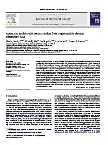
Figure 2.4 shows a schematic view of the algorithm we have just employed on examples in the two previous sections. In section 2.1 we focused on the high-level view, shown in �g. 2.4a and detailed in chapter 6. It begins with an initial control �ow fragment
C
and an initially empty resolver
each iteration, it picks a CFG node
v
R.
In
with yet unknown successors, and
computes the successor locations. With the knowledge gathered in this step, it expands the CFG by adding successor nodes. Furthermore, it sometimes di�erentiates between traces that were previously treated equally, i.e., ended up in the same CFG node, by splitting this CFG node if it discovers that in a future step, these traces exhibited di�erent control �ow behaviour. 20
2.3.
A SCHEMATIC ALGORITHM
Figure 2.4b displays the resolution of a single CFG node
v
as demon-
strated in section 2.2, an adaptation of the classical trace abstraction re�nement loop, formally described in chapter 5. It must consider the instruction
v in all possible contexts, i.e., preceded by all traces ρp that reach v in the current CFG fragment. Therefore it takes as input the lanp that consist of such a ρp followed by the respective guage Lv of all traces τ instruction of v . It aims to build a resolver automaton Rv , that accepts all at node node
these, and possibly more, traces. To this end, it picks in each iteration a not yet accepted trace, computes the locations and an inductive sequence. From this sequence, it builds a generalization in the form of a resolver is added to the accumulated
Rv .
Once the language
Lv
Rτp ,
which
is covered by
the loop terminates and the resolver is returned. In our example,
τp3
Rv ,
was the
�rst analysed trace � the case of a single loop iteration �, and the computed resolver
Rτp3
shown in �g. 2.3 already covers
Lv ,
i.e., it accepts traces with
an arbitrary number of loop iterations. In fact, it accepts even more traces, including the trace that skips the loop entirely, and traces containing the loop body instructions in di�erent orders. Hence the returned resolver exactly
Rτp3 .
21
Rv
is
CHAPTER 2.
CONTROL FLOW RECONSTRUCTION: OVERVIEW
22
Chapter 3
Basic De�nitions This chapter gives a number of formal de�nitions describing the setting of binary programs. These are then used to formalize the requirements in the next chapter, and as a basis for the reconstruction approach.
Before we
begin, let us �x a few notational conventions:
•
Unless otherwise stated,
n P N0 .
• f : M ã N denotes a partial function f from set M to formula f pxq “ K means that f is unde�ned for value x. •
empty sequence. For two sequences denoted as
3.1
The
M ˚ for any set M in M . ε denotes the
w1 , w2 P M ˚ ,
the concatenation is
w1 ¨ w2 .
f1 : M1 Ñ N1 , f2 : M2 Ñ N2 with M1 X M2 “ H, f1 ‘ f2 : M1 Y M2 Ñ N1 Y N2 denotes the function de�ned by # f1 pxq if x P M1 pf1 ‘ f2 qpxq “ f2 pxq otherwise
For functions
Instruction Sets
Machines V
N.
As common when dealing with formal languages, denotes the set of �nite sequences of elements
•
set
Our setting is a machine
and memory locations
the program counter.
D
Loc.
M “ pV, pc, Loc, Dq
with variables
pc P V , v P V , with
We distinguish a special variable
is a family of domains
Dv
for each
Dpc “ Loc.
Example 3.1 a machine
•
.
(ARM Processor)
We will model a 32bit ARM processor as
MARM “ pV, pc, t0, 1u32 , Dq.
registers
r P t r0, . . . , r15 u
with
23
The variables
Dr “ t0, 1u32 ,
V
are split into
CHAPTER 3.
BASIC DEFINITIONS
•
comparison �ags
f P tN, C, Z, Vu
•
and the memory
mem
with
Df “ t0, 1u,
with
Dmem “ t0, 1u32 Ñ t0, 1u8 .
The program counter is to by the name
pc “ r15. r14 is the link return register, also referred lr. The stack pointer is sp “ r13.
M is given v P V . State is the
A state of for all
s:V Ñ
by a mapping
Ť vPV
Dv ,
with
spvq P Dv
set of all such states.
Instruction Sets
An instruction set for
a set of instructions
I
and their semantics
M is given by a tuple pI, v¨wq of v¨w : I Ñ State ã State. An in-
struction in this context contains not only the operator, but also the operand speci�cation, for instance a constant, or a variable in an instruction
ι P I , vιw,
Example 3.2
(AArch32 Instruction Set)
V.
The semantics of
are given by a partial function between states.
.
The AArch32 instruction set for
ARM processors [4] contains a large number of di�erent instructions, such as data processing instructions operating on registers and constants, load/store instructions for transferring data between registers and the memory, and direct as well as indirect branch instructions (jumps) for control �ow. In contrast to many other instruction sets, it has conditionally executed
variants not only for branch instructions, but most data processing instructions as well. Comparison instructions such as set the condition �ags
N, C, Z
and
V.
cmp
compare operands and
Subsequent instructions can have a
condition code to control their execution. For instance
addeq
only executes
an addition if the last comparison had two equal operands, or
bgt
only
branches to its target address if the �rst operand of the previopus comparison was larger than the second. If the condition of such an instruction is violated, it behaves like a
nop instruction, solely incrementing pc by 4 bytes.
A partial function is suited because a state may have no successors. For instance, an instruction like
halt
may assign no successor to any state. As
an other example, the indirect branch instructions in ARM such as
bx r0 are
only de�ned for branch targets aligned to word boundaries, i.e., divisible by 4. By representing the instruction semantics as a partial function, we limit ourselves to deterministic instructions. However, the presented framework is easily adapted to nondeterministic instructions (e.g. for dealing with user input) by replacing the partial function with a binary relation. Unless otherwise indicated, we will in the remainder assume a �xed instruction set
Traces I ˚.
A
We call
K “ pI, v¨wq
K -trace is τ feasible
for our machine
M.
a �nite sequence of instructions
τ “ pι1 , . . . , ιn q P σ “
i� there is a corresponding sequence of states 24
3.1.
INSTRUCTION SETS
ps1 , . . . , sn`1 q P State˚ so that si`1 “ vιi w psi q is de�ned for all i P t 1, . . . , n u. If such a σ exists, it is a witness for τ , written σ $ τ . Otherwise, τ is infeasible. InfeasK denotes the set of all infeasible K -traces. Note that the empty trace ε is always feasible (no matter the semantics), and that InfeasK is a right-ideal, i.e., if a trace τ is infeasible, so are all 1 traces τ ¨ τ .
Location-Aware Instruction Set
Given an instruction set
we can derive another instruction set for
M.
K “ pI, v¨wq,
We will make use of this derived
instruction set during control �ow reconstruction. Typically, the instructions in an instruction set supported by a processor have no knowledge of their location.
However, they implicitly de�ne
their own control �ow by the way they manipulate
pc.
We can add this
information to the instructions explicitly:
De�nition 3.1 (Location-Aware Instruction Set) �
aware instruction set as Kp “ pLoc ˆ I, v¨wq with # vpl, ιqw psq “
The semantics veri�es that the
location-
vιw psq ‰ K ^ sppcq “ l
if
vιw psq K
We de�ne the
otherwise
pc
is equal to the instruction's location,
and then behaves just as the instruction
ι
would. However, in states where
this check fails, there is no successor state. As a notational convention, we separate a location from an instruction by a colon, i.e., we write of
pl, ιq.
τp “ pl1 : ι1 , . . . , ln : ιn q, pι1 , . . . , ιn q simply by τ .
Given a location-aware trace
corresponding
K -trace
l:ι
in place
we refer to the
Let us examine the possible reasons for the infeasibility of a location-
τp “ pl1 : ι1 , . . . , ln : ιn q. Clearly, τp is infeasible if and only if there is some index i P t 1, . . . , n u, such that the trace pre�x pl1 : ι1 , . . . , li´1 : ιi´1 q always establishes a state s in which li : ιi can not execute, i.e., vli : ιi w psq “ K. This in turn can mean the location is incorrect, sppcq ‰ li , or the original instruction can not execute, vιi w psq “ K, or both. aware trace
Example 3.3
.
(Reasons for Infeasibility)
Let us consider the following
location-aware traces:
0000: mov r0 , #42 0004: ldr r1 , [ r0 ] 0008: nop Listing 3.1:
0000: bl 0020 0020: bx lr 0024: nop Listing 3.2:
Unaligned memory access.
The trace in listing 3.1 �rst sets register
r0
Incorrect return.
to the constant value 42.
It
then attempts to load data from that memory location, storing the value
25
CHAPTER 3.
in register
r1,
is to increase
BASIC DEFINITIONS
and �nally performs a non-operation
pc
by 4.
nop,
whose only e�ect
However, the AArch32 instruction set only allows
memory reads at word boundaries, i.e., at addresses that are a multiple of 4. Loading from an unaligned address such as 42 invokes unde�ned behaviour [4].
Therefore this trace is infeasible.
This has nothing to do with the
fact that it is a location-aware trace, in fact the corresponding
K -trace
is
infeasible as well. Hence the infeasibility stems from a condition imposed by the original AArch32 instruction set. In this aspect, it di�ers from the second trace in listing 3.2, which is
0000 to location location 0004 (the
infeasible as well. It performs a direct branch from location
0020
(hexadecimal), while setting
e�ect of in
lr,
bl).
lr
to the subsequent
It then returns via an indirect branch to the value stored
and �nally performs a
nop.
This is in itself perfectly feasible. The
infeasibility stems from the fact that the non-operation is located at address
0024, whereas any state s reached after execution of the �rst two instructions must have sppcq “ 0004. Hence the infeasibility stems from the condition added by the location-aware instruction set.
0000: 0004: 0020: 0024:
mov bl bx ldr
r0 , #42 0020 lr r1 , [ r0 ]
Listing 3.3:
Incorrect return and unaligned memory access.
Lastly, both these causes of infeasibility can occur simultaneously in a trace, such as the one given in listing 3.3.
The trace pre�x consisting of
only the �rst three location-aware instructions is feasible.
However, the
last location-aware instruction cannot execute in a state established by this pre�x: The location-check of the location-aware semantics will fail, because the instruction is located at location
0024, whereas pc must be 0008.
At the
same time, the instruction would attempt to read from an unaligned address.
3.2
Programs
So far, we have only discussed instruction sets and properties of their semantics, without any notions of programs. As we will construct control �ow graphs for speci�c programs, we need a formal de�nition of programs:
De�nition 3.2
(Program)
�
A
K -program p “ pLocp , linit , instr , Sinit q
given as a tuple of
•
a �nite set of program locations
Locp Ď Loc,
26
is
3.2.
•
an initial location linit
•
a mapping
•
and a set of possible initial states
PROGRAMS
P Locp ,
instr : Locp Ñ I
from program locations to instructions,
Sinit ‰ H,
such that
Sinit Ď t s P State | sppcq “ linit u By this de�nition, the instruction at a memory location is �xed and we thus do not consider programs modi�ed at runtime. Refer to the discussion of future work in section 10.4 for thoughts on how to extend the approach for self-modifying code.
Example 3.4
(An ARM program)
.
The following listing shows a small
AArch32 program counting from 0 to 255:
0000: 0004: 0008: 000 c: 0010: 0014: 0018: 0020:
ldr r1 , [ pc , #24] mov r0 , #0 b 0010 add r0 , r0 , #1 cmp r0 , r1 bne 000 c b 0018 . word 0 xFF Listing 3.4:
Written as a tuple
; ; ; ; ; ; ; ;
load word 0 xFF into r1 initialize r0 to 0 goto 0010 ( enter loop ) increment r0 compare r0 and r1 if unequal , goto 000 c halt stored constant 255
A program counting to 255.
p “ pLocp , linit , instr , Sinit q,
this program has
• Locp “ t0000, 0004, 0008, 000c, 0010, 0014, 0018u, • linit “ 0000, •
a mapping
•
and
instr
as given by the listing above (ignoring the last line),
Sinit “ t s P State | sppcq “ 0000 ^ spmemqp0020q “ 0xFF u
Note that the initial states are restricted to those that store the constant 255 at location
0020.
This is important as correctness and control �ow of the
program may depend on such values. In particular, switches are sometimes encoded by including branch addresses as constants (in so-called jump tables ) and then dynamically loading them into
pc.
In the remainder of the thesis, we will assume a �xed
pLocp , linit , instr , Sinit q
without further mention.
the set of all instructions in a program, so we de�ne here: 27
K -program p “
We will need to refer to
CHAPTER 3.
BASIC DEFINITIONS
De�nition 3.3 and the
(Program Alphabets)
�
We de�ne the
location-aware program alphabet as
program alphabet
Σppq “ im instr “ t instr plq | l P Locp u and
p Σppq “ t l : instr plq | l P Locp u p Σppq and Σppq to refer to the corresponding instruction sets, p , respectively. with the instructions as above and the semantics as in K and K We will also use
Note that
z: p Σppq ‰ Σppq
The �rst contains only pairs of locations and
instructions as de�ned in the program, whereas the latter contains the instructions of the program paired with arbitrary locations.
De�nition 3.4
(Program Witnesses, Executions)
�
A location-aware trace
τp “ pl1 : ι1 , . . . , ln : ιn q is a location-aware p-trace if and only if it is a p -trace and there is a sequence of states σ “ ps1 , . . . , sn`1 q such that Σppq σ $ τp and s1 P Sinit . In this case we say σ is a p-witness for τp, written σ $p τp. Eppq, the set of executions of p is the set of all p-witnesses. Based on this de�nition, we can de�ne the language of a program:
De�nition 3.5 (Program Languages) � p
The
location-aware language of
is
p “ t τp P Σppq p ˚ | Dσ . σ $p τp u Lppq The
language of p is p u Lppq “ t τ | τp P Lppq
Control Flow
p captures the program behaviour precisely. Note that any p-witness for τ p is a witness p, and thus the existence of a p-witness for τp implies that τp is feasible. for τ p and Lppq are feasible. However, this is sometimes Therefore all traces in Lppq The (location-aware) language of a program
too strict, too precise for our purpose.
Similar to control �ow graphs for
structured programs, we want to extract a notion of the control �ow from the behaviour of
p;
a weaker, less precise notion that does not imply feasibility.
Since control is transferred through modi�cations of
pc, it is natural that we
are interested in its possible values after execution of a trace:
De�nition 3.6 set of possible
(Successor Locations)
p-successor
�
Let
τp
locations of τp as
be a
p -trace. K
We de�ne the
loc p pp τ q “ t l P Locp | Dps1 , . . . , sn`1 q . l “ sn`1 ppcq ^ ps1 , . . . , sn`1 q $p τp u 28
3.2.
PROGRAMS
This gives us a set of locations. For many traces, there is only a single possible value of
pc,
but in some cases there may be more than one, e.g.
if the last instruction is a conditional branch, or an indirect branch to an address loaded from a jump table. Moreover, for a trace
loc p pp τ q “ H.
p , τp R Lppq
we have
The following de�nition uses this set of locations to give a
notion of a program's control �ow:
De�nition 3.7
(Control Flow Conformance, Control Flow Errors)
�
Let
p -trace. For k P t 0, . . . , n u let τp|k denote the τp “ pl1 : ι1 , . . . , ln : ιn q be a Σppq p conforms to the control �ow of p i� pre�x pl1 : ι1 , . . . , lk : ιk q. Then τ p @k P t 0, . . . , n ´ 1 u . τp|k P Lppq ùñ lk`1 P loc p pp τ |k q If this is not the case,
τp
is said to have a
control �ow error (CFE).
At �rst, this notion of control �ow seems weak in the sense that, once a pre�x of
τp
is not in
trace are arbitrary. is always in
p . Lppq
p , Lppq
the subsequent locations and instructions in the
However, the shortest pre�x, i.e., the empty trace
In order for a control �ow conformant trace to �leave�
p , there must be a pre�x τp|k that always Lppq vιk`1 w psq “ K, for all initial states in Sinit .
Theorem 3.8 �
ε,
establishes a state
s
where
p -trace that conforms to τp “ pl1 : ι1 , . . . , ln : ιn q be a Σppq p . Then there is a k P t 0, . . . , n ´ 1 u p R Lppq the control �ow of p, such that τ p such that τ p|k P Lppq and for all σ “ ps1 , . . . , sk`1 q with σ $p τp|k where sk`1 ppcq “ lk`1 (by conformance, there is at least one such σ ), we have vιk`1 w psk`1 q “ K. Let
|p τ | of the trace. The empty trace ε p is always in Lppq. We can thus assume that τ p is a non-empty trace τp “ p p conforms to the control pl1 : ι1 , . . . , ln`1 : ιn`1 q, such that τp R Lppq and τ p “ pl1 : ι1 , . . . , ln : ιn q also conforms to the control �ow of p. Then the pre�x ρ p , the result follows by induction. p R Lppq �ow of p. Thus, if ρ p . Let σ “ ps1 , . . . , sn`1 q such that σ $p ρp and Suppose ρ p P Lppq p . sn`1 ppcq “ ln`1 . If vιn`1 w psn`1 q ‰ K, then vln`1 : ιn`1 w ‰ K and τp P Lppq Since this contradicts the assumption, we have vιn`1 w psn`1 q “ K. Thus we set k “ n P t 0, . . . , pn ` 1q ´ 1 u. Proof. By induction over the length
The essence of this theorem is that if a trace conforming to the control
p , the reason for this is always a violated condition of the p is not in Lppq original instruction set K , not incorrect control �ow violating the location�ow of
check introduced by the location-aware semantics (cf. example 3.3).
29
CHAPTER 3.
BASIC DEFINITIONS
30
Chapter 4
Capturing Control Flow Our goal is to reconstruct the control �ow from a binary program. This has many applications in di�erent �elds, from decompilers, over security analysis to analysis of properties such as worst-case execution time. Before we begin developing an algorithm, we �rst state the form our result will take and propose some quality requirements it should satisfy.
4.1
Properties of Control Flow Graphs
Instead of de�ning a single target graph, we de�ne a very general class of control �ow graphs.
We will subsequently characterise certain properties
sensible control �ow graphs should satisfy.
De�nition 4.1
(Control Flow Graph (CFG))
�
(CFG) for program p is a tuple pV, Vinit , E, `q of •
a set of nodes
•
a set of initial nodes
•
a set of edges
•
and a node labeling function
A
control �ow graph
V, Vinit Ď V ,
E ĎV ˆV, ` : V Ñ Locp .
A key di�erence from existing control �ow reconstruction approaches is that we do not have a one-to-one association between CFG nodes and program locations. Each node has a unique associated program location, but there may very well be multiple nodes associated with the same location. In fact, this will be key to one of the desired properties discussed below.
In
order to formalize these properties, let us �rst de�ne the language of a CFG: 31
CHAPTER 4.
CAPTURING CONTROL FLOW
De�nition 4.2 K -program p.
� Let C “ pV, Vinit , E, `q p -trace τp “ pl1 : ι1 , . . . , ln : ιn q is accepted K ˚ nodes pv1 , . . . , vn`1 q P V such that (CFG-Languages)
A
is a sequence of 1.
v1 P Vinit
is the initial location,
2.
`pvi q “ li
and
3. and
instr pli q “ ιi
pvi , vi`1 q P E
for all
C
C
i� there
i P t 1, . . . , n u,
i P t 1, . . . , n u
location-aware language p p. The language of C is the LpCq is the language of all such traces τ
If this is the case, we write
of
for all
be a CFG for by
τp
v1 Ý Ñ vn`1 .
language of the corresponding
C
The
K -traces
p LpCq “ t τ | τp P LpCq u We shall now introduce the mentioned requirements for sensible control �ow graphs. Throughout, we will assume a CFG program
C “ pV, Vinit , E, `q
Requirement 1
(Finiteness)
�
The control �ow graph should be �nite. (4.1)
|V | ă 8 If
C
C
is �nite, the set of accepted traces
can serve as a �nite automaton.
want
C
for the
p.
p LpCq
is a regular language, and
Less formally, but still important, we
to not only be �nite but have a reasonable size.
Naturally, not any �nite graph is acceptable. At the very least, we want the CFG to over-approximate the control �ow of
p.
This will allow us to
perform static analyses such as veri�cation on the CFG while avoiding false negatives: If all traces of
Requirement 2
C
satisfy some criterion, then so do all traces of
(Correctness)
�
p.
The control �ow graph should be correct,
i.e., it should over-approximate the possible program traces.
p Ď LpCq p Lppq
(4.2)
While we do create an over-approximation as per requirement 2, requirement 3 restrains this again:
The over-approximation should not be
too coarse, otherwise a simple automaton accepting all syntactically possible traces of an instruction set would be admissible as CFG. The CFG should accurately represent our notion of control �ow de�ned in de�nition 3.7. It is the ful�llment of this requirement (under some su�cient conditions) that 32
4.1.
PROPERTIES OF CONTROL FLOW GRAPHS
distinguishes our approach from established techniques. This additional precision reduces the workload for static analyses working on the CFG by eliminating the need to analyse a large number of traces only to discover they do not accurately represent the control �ow of the program.
Requirement 3
(Freedom from Control Flow Errors)
�
The CFG should
not accept traces that have control �ow errors (cf. de�nition 3.7). Equivalently, all accepted traces should conform to the control �ow of
p.
While this seems like a suitable requirement for a CFG, it is di�cult to verify. In order to simplify this, we give a su�cient condition:
De�nition 4.3 CFG for
p,
C -successor
�
(CFG Successor Locations)
τp “ pl1 : ι1 , . . . , ln : ιn q locations of τp is given as
and let
be a
Let C “ pV, Vinit , E, `q be a p -trace. The set of possible K
τp
τ q “ t l P Locp | Dv P Vinit , v 1 P V . v Ý Ñ v 1 ^ `pv 1 q “ l u loc C pp C
Theorem 4.4 program
p.
(CFE-free CFGs)
�
Let
C “ pV, Vinit , E, `q
be a CFG for
If
p p . loc C pp τ P LpCq @p X Lppq τ q Ď loc p pp τq then all traces
p τp P LpCq
conform to the control �ow of
(4.3)
p.
p , and let τp “ pl1 : ι1 , . . . , ln : ιn q P LpCq p , and k P t 0, . . . , n ´ 1 u. The pre�x τp|k “ pl1 : ι1 , . . . , lk : ιk q is also in LpCq p by the de�nition of LpCq we know that lk`1 P loc C pp τ |k q. Thus if furthermore p , we conclude by eq. (4.3) that lk`1 P loc p pp τp|k P Lppq τ |k q. Proof. Assume eq. (4.3) holds. Let
This su�cient condition is even necessary, provided every accepted trace is a strict pre�x of another accepted trace.
While this is not a sensible
requirement, and even correct CFGs may violate it, it serves to demonstrate the close connection between requirement 3 and eq. (4.3).
Lemma 4.5 �
C “ pV, Vinit , E, `q be a CFG for program p. If for every p v P V , there is a v P V such that pv, v 1 q P E , and all traces τp P LpCq conform to the control �ow of p, then eq. (4.3) holds. Proof. Let
Let 1
p p . τp P LpCq X Lppq
vP
Vinit and a node v 1
is a
v2 P V
with
PV
As it is accepted by
C,
there is an initial node
vÝ Ñ
v 1 . Then by assumption, there
and therefore
` ˘ p . τp ¨ `pv 1 q : instr p`pv 1 qq P LpCq control �ow of p, and therefore
such that
pv 1 , v 2 q P E ,
τp
C
By assumption, this trace conforms to the 33
CHAPTER 4.
CAPTURING CONTROL FLOW
p τp P Lppq
its pre�x
τ q. Thereby `pv 1 q, i.e., `pv 1 q P loc p pp τ q, we also have l P loc p pp τ q. l P loc C pp
correctly predicts
have shown that for an arbitrary
we
Seeing as our requirements demand a regular language (by requirement 1) that over-approximates
p Lppq
(by requirement 2), but not too coarsely (by
requirement 3), one might be tempted to go further and require a minimal regular over-approximation of
p . Lppq
However, such a solution does not in
the general case exist:
Lemma 4.6 � language
Lmin
If
L
is not a regular language, there is no
over-approximating
Lmin zL ‰ H, as L not regular But then for any non-empty, �nite Lfin Ď Lmin zL, there is over-approximation Lmin zLfin Ă Lmin of L.
Proof. Assume such a language by assumption. a better regular
minimal regular
L.
Lmin
existed.
The language of program traces is in many cases not regular. But even in cases where it is, a CFG accepting exactly the program language is not necessarily the result one would intuitively expect:
Example 4.1 (Exact CFGs are sometimes undesirable).
Let us consider the
following program:
0000: bl 0004: b
0020 0004
; set lr = 0004 , goto 0020 ; halt
0020: 0024: 0028: 002 c: 0030:
r0 , #0 r0 , r0 , #1 r0 , #10000 0024 lr
; ; ; ; ;
mov add cmp bne bx
Listing 4.1:
set r0 = 0 increment r0 compare r0 to 10 000 if unequal , goto 0024 goto value of lr (0004)
An example loop program.
It consists of a simple loop counting from 0 to 10 000. capturing
Lppq
for this program
p
A CFG precisely
would look as in �g. 4.1a: It unrolls the
loop and thus only accepts the one actual program trace. However, this level of accuracy is not what is desired in a control �ow graph � data properties such as the truth of the loop condition are not usually considered part of the control �ow. The expected CFG is shown in �g. 4.1b. It sacri�ces accuracy by accepting traces with an arbitrary number of iterations. Therefore, it needs much fewer states.
34
4.1.
PROPERTIES OF CONTROL FLOW GRAPHS
0000 mov r0,#0 0004
0004
add r0,r0,#1 0008
0004 add r0,r0,#1
(not z) / b 0004
cmp r0,#10000
...
0008
cmp r0,#10000 (not z) / b 0004
000C
(a)
(not z) / b 0004 add r0,r0,#1 0008
0010
b 0010
cmp r0,#10000 (not (not z)) / nop
000C
000C
In a precise CFG, the loop is unrolled. The CFG accepts only one trace.
add r0,r0,#1 mov r0,#0
0000
(b) Figure 4.1:
0004
0008
b 0010
cmp r0,#10000
(not z) / b 0004
000C
(not (not z)) / nop
0010
The expected CFG accepts an arbitrary number of iterations.
Precise and expected CFG for a loop with a minimum number of iterations.
It is an as yet open question for which programs a CFG satisfying all these requirements, in particular requirement 3, even exists. For instance, recursive programs typically compile to assembler programs for which no such CFG exists. Confer to chapter 10 for some discussion of this limitation.
Example 4.2 (Recursion and CFEs).
As an example of a program for which
no CFG satisfying requirements 1 to 3 exists, consider the following recursive program.
0000: bl 0004: b 0020: 0024: 0028: 002 c: 0030: 0034:
0020 0004
; set lr = 0004 , goto 0020 ; halt
cmp r0 , #0 ; compare r0 to 0 bxeq lr ; if r0 = 0 , return sub r0 , r0 , #1 ; decrement r0 push { lr } ; push lr on stack bl 0020 ; set lr = 0034 , goto 0020 pop { pc } ; pop stack into pc Listing 4.2:
An example loop program.
35
CHAPTER 4.
CAPTURING CONTROL FLOW
0020, which recursively decrements r0 until it reaches 0. Once this termination condition is reached, the function returns (location 0024). As long as it does not hold, r0 is decremented, the It contains a function, located at location
return address is pushed on the stack, and the function recurses (location
0030).
When the recursive call returns, the return address previously stored
on the stack is popped directly into
pc.
This is e�ectively an indirect branch
to an address loaded from memory. A correct, CFE-free CFG
C
for this program would e�ectively have to
keep count of the recursion depth, or even the call stack: Given two traces
τpn , τx m that both end up in location 0024, with a recursion depth of n resp. m with m ą n, suppose they both reached the same node v 1 in in C . Then 1 and the trace τx ¨ τp1 would be accepted by C and both the trace τpn ¨ τpn m n 2 1 consists of n repetitions of the pop again reach the same node v , where τpn 1 , v 2 must be labeled instruction at location 0008. But by correctness for τpn ¨ τpn 0004, as the recursion depth is 0. At the same time, by CFE-freedom for p1 τx m ¨ τn , the only acceptable label would be 0034, as the recursion depth is 1 m ´ n ą 0. Hence, τpn and τx m cannot reach the same node v . But then the 1 CFG nodes vn reached by all traces τpn for all possible recursion depths n must be distinct. Therefore C violates requirement 1.
4.2
Possible Control Flow Graphs
In this section we consider some possible control �ow graphs for a program
p,
and discuss how they satisfy or violate the requirements. By de�nition, the
pc
after every instruction is completely determined by
the instruction and the previous machine state.
Therefore, observing the
entire machine state in each step gives us the most precise CFG possible:
De�nition 4.7 (Precise CFG T ppq) � p
is de�ned as
T ppq “ pS, Sinit , E, `q
The
precise control �ow graph of
with nodes
S “ t s P State | sppcq P Locp u labeled by
`psq “ sppcq
and edges
E “ t ps, vιw psqq | s P S ^ ι “ instr psppcqq u This CFG trivially ful�lls requirements 2 and 3, as it accepts exactly
p ppqq “ Lppq p . LpT
Of course, depending on the machine, it is in�nite or at
least inacceptably large, violating requirement 1. In order to have a �nite model, we need to give up some of the precision a�orded by observing the entire machine state, thus reducing the number of nodes while accepting 36
4.2.
POSSIBLE CONTROL FLOW GRAPHS
more traces. In fact, control �ow analysis in structured programming languages usually ignores state information completely, focussing on the program's structure only. However, when analysing binary programs, i.e., unstructured code, we cannot a�ord this luxury: Control �ow and data �ow are inseparably intertwined via the
pc variable.
We thus have to �nd a com-
promise. One approach is to only take into account the current value of as for most instructions this already determines the next
pc.
pc,
This results in
the following de�nition:
De�nition 4.8 (pc-CFG) �
The
CFG pc ppq “ pLocp , t linit u, E, idq
pc-based
CFG of a program
p
is de�ned as
with
E “ t psi ppcq, si`1 ppcqq | ps1 , . . . , sn`1 q P Eppq ^ i P t 1, . . . , n u u Note that this or similar de�nitions are very common in the literature, e.g. [5, 6]. The states in this CFG are given by program locations, hence it is �nite and the generated language is regular (requirement 1). easily be seen that this CFG further satis�es requirement 2. The
It can
pc-based
CFG rejects some infeasible traces, such as dead code that cannot be reached due to e.g. an unsatis�able branch condition. On the other hand, it does accept some infeasible traces based on inconsistent reads and writes of
pc:
For instance, consider again the example in section 2.1, where a function is called twice from two di�erent locations. The
pc-based
CFG would accept
all traces leading from a call at call site A through the function and its return statement to any call site B, i.e., the CFG would be as shown in �g. 2.2c (including the dashed edge and node).
This violates requirement 3.
This
behaviour is opposite to the control �ow analysis in a structured program, where a dead branch would be explored but an incorrect return would be recognized as impossible, either through function inlining or a combined approach of intraprocedural CFGs and a call graph. Hence this de�nition has accurracy where it might not be needed, but lacks it where it would be expected. It turns out that, in order to meet our requirements, it is insu�cient to only observe the
pc.
On the other hand, we already remarked that observing
the entire machine state does not yield a solution either. Nor is it feasible to statically identify a small subset of the state information that will su�ce while still being reasonably small. Thus we need a method to dynamically, depending on the program, capture state information that will su�ce to predict future
pc
values.
This is exactly what we can achieve using trace
abstraction re�nement.
37
CHAPTER 4.
CAPTURING CONTROL FLOW
38
Chapter 5
Resolving Traces As we have seen in chapter 2, a key element in the control �ow reconstruction algorithm will be the ability to determine possible locations after the
τp, loc p pp τ q as given in de�nition 3.6. Our result will in Ω such that loc p pp τ q Ď Ω for the given trace τp: While we can
execution of a trace general be a set
compute exact results for a single traces, in order to generalize these results to multiple traces, a loss of exactness must be tolerated. Let's say we have determined a set of successors
loc p pp τq Ď Ω
for a given trace
τp.
Ω Ď Loc
such that
We want to generalize this result to more
traces. For this purpose, we de�ne a notion of a proof of this result, which can then be used to conduct analogous proofs for similar traces and even to derive more complex proofs. This de�nition is adapted from trace abstraction re�nement approaches to veri�cation as presented in [7].
De�nition 5.1
�
pτp “ pl1 : ι1 , . . . , ln : ιn q be a K trace, and let Ω Ď Loc. A sequence of sets pS1 , . . . , Sn`1 q (Si Ď State) is a location-inductive sequence (or simply inductive sequence) for pΩ, τ pq (Inductive Sequence)
Let
i� the following conditions hold:
Sinit Ď S1
(5.1)
t vli : ιi w psq | s P Si ^ vli : ιi w psq ‰ K u Ď Si`1
(5.2)
Sn`1 Ď t s P State | sppcq P Ω u where
(5.3)
i P t 1, . . . , n u.
This sequence provides some information about �rst state of such a
p-witness
p-witnesses
of
τp:
The
must be a valid initial state of the program
(eq. (5.1)), the witness follows the trace (eq. (5.2)), and the last state of the
p-witness
must have one of the computed locations (eq. (5.3)).
minimal inductive sequence would be
Si “ t si | ps1 , . . . , sn`1 q $p τp u.
choosing larger sets, the proof is generalized: 39
The By
Sequences of large sets are
CHAPTER 5.
RESOLVING TRACES
inductive sequences for more traces. The goal is to only include information that is necessary to prove the end result. The existence of such an inductive sequence does indeed amount to a proof of our result, as shown by the following theorem:
Theorem 5.2 some
(Inductive Sequences as Proofs)
Ω Ď Loc
�
Let
there exists an inductive sequence for
p -trace. If for τp be a K pΩ, τpq, then loc p pp τq Ď
Ω. τp “ pl1 : ι1 , . . . , ln : ιn q and σ “ ps1 , . . . , sn`1 q such that σ $p τp. τ , Ωq. By de�nition of pS1 , . . . , Sn`1 q be an inductive sequence for pp witnesses and induction over i it follows that si P Si for all i P t 1, . . . , n`1 u. Therefore sn`1 P Sn`1 and thus the conclusion follows. Proof. Let Let
loc p pp τ q Ď Ω, pp τ , Ωq, an we can construct it in a standard manner. This process of computing Ω and �nding an inductive sequence for τ , Ωq will be referred to as resolving τp. pp As we will see below, the reverse of theorem 5.2 also holds: If
there is an inductive sequence for
5.1
Handling Simple Instructions
By the de�nition of program traces, an instruction determines the next instruction to be executed by setting the program counter
pc
accordingly.
While most instructions in practice simply set it to the location of the logically subsequent instruction, some instructions (branches) exhibit a more complex behaviour.
The following de�nition of an instruction's successor
degree classi�es instructions by this complexity: It gives the maximum number of di�erent successor locations, provided the instruction's own location is known.
De�nition 5.3 struction. The
(Successor Degree, Simple Instructions)
successor degree of ι is de�ned as
�
Let
ι
be an in-
degpιq “ sup |t vιw psqppcq | s P State ^ sppcq “ l ^ vιw psq ‰ K u| lPLoc
degpιq “ 8 if no such supremum exists, and of course sup H “ 0. Instructions ι with degpιq ď 1 are called simple instructions.
We write
Example 5.1 (Simple Instructions in ARM).
In ARM, most data processing
instruction types such as addition (add), subtraction (sub), assignment (mov) etc. are simple instructions � unless their output register is but legal [4]).
pc (deprecated For instance, add r0, r1, #4 is simple, but add pc, r1, #4 40
5.1.
HANDLING SIMPLE INSTRUCTIONS
b 0020, are also simple; whereas bx lr, are not. Strictly speaking, a conditionally executed direct branch, e.g. beq 0020,
is not. Direct branch instructions, such as
indirect branches, such as the typical �return�
is not a simple instruction simple either: For some (in fact, for any) �xed
l P Loc, there are states s1 , s2 P State such that s1 ppcq “ s2 ppcq “ l and vbeq 0020w ps1 q ‰ K, vbeq 0020w ps2 q ‰ K, but in s1 the comparison �ags satisfy the condition, i.e., s1 pN q “ 1, whereas in s2 they do not, i.e., s2 pN q “ 0. Therefore degpbeq 0020q ą 1 (speci�cally degpbeq 0020q “ 2). However, in section 8.2, we will see how to handle such a conditional instruction as two alternatives, b 0020 and nop; both of which are simple location
instructions. For a simple instruction, we can determine statically the successor location after executing the instruction, given only the instruction's own location. In other words, such an instruction de�nes a partial function:
De�nition 5.4 tion.
Then the
(Unique Successor Function)
�
unique successor function of
successor ι : Loc ã Loc
ι
Let
ι
be a simple instruc-
is the partial function
characterized by
@s P State . vιw psq ‰ K ^ sppcq “ l ðñ vιw psqppcq “ successor ι plq for all
l P Loc.
This partial function can be used to resolve location-aware traces
pl1 : ι1 , . . . , ln : ιn q
where
ιn
τp “
is a simple instruction. The construction of an
inductive sequence is simple:
Lemma 5.5 trace
(Inductive Sequence for Simple Instructions)
τp “ pl1 : ι1 , . . . , ln : ιn q
with
ną0
and
degpιn q ď 1,
and
�
Given a
Ω Ď Loc
pK
such
that
successor ιn pln q ‰ K ùñ successor ιn pln q P Ω Then an inductive sequence for
pp τ , Ωq
is given by
Si “ State Sn`1 “ t s P State | sppcq P Ω u where
i P t 1, . . . , n u.
While this resolution strategy only applies to a subset of traces, it can be implemented very e�ciently. In the cases where it can not be applied, we can fall back to the more complex resolution strategies presented in the remainder of the chapter. 41
CHAPTER 5.
5.2
RESOLVING TRACES
SMT-Based Location Computation
In order to resolve traces ending in non-simple instructions, we have to take into account the context established by the entire trace. This can be done by encoding the trace in �rst-order formulae, as demonstrated in chapter 2 (eqs. (2.1) and (2.2)), and using an SMT solver to compute possible solutions.
Encoding Traces
In order to encode a trace in formulae, we need to
convert it to static single assignment (SSA) form, where each variable is only assigned once. This is a common step of trace abstraction re�nement techniques, and is typically done via indexing, e.g. de�nition, the index of
τp “ pl1 : ι1 , . . . , ln : ιn q
v P V
in [7].
Adapting this
i P t 1, . . . , n ` 1 u
at position
in a trace
is given by
$ ’ &1 ϑi pvq “ ϑi´1 pvq ` 1 ’ % ϑi´1 pvq
if if
i“1 ιi´1 de�nes v
otherwise
v i� there is a state s such that vιw psq ‰ K and spvq ‰ vιw psqpvq. We assume the semantics vιw of instructions ι can be given as a pair pδι , µι q of a formula δι over variables in V , and a mapping µι from V to terms over V , such that for all states s P State, where we say that an instruction de�nes
vιw psq ‰ K ðñ s |ù δι and furthermore, if
(5.4)
vιw psq ‰ K, vιw psq “ s ˝ µι
(5.5)
Note that we are here treating machine states over variables
V,
and that
sptq
for a term
t
s
as �rst-order valuations
over variables in
V
denotes
t under valuation s. The same principle is used Sinit by a set Φinit of formulae over V . The following set Φpp τ q then encodes the trace τp:
the semantics of term
to
characterize
of
formulae
Φpp τ q “ Φinit rϑ1 s Y t διi rϑi s | i P t 1, . . . , n u u Y t vϑi`1 pvq “ µιi pvqrϑi s | i P t 1, . . . , n u ^ ιi
de�nes
vu
Y t pcϑi ppcq “ li | i P t 1, . . . , n u u
(5.6)
ϑi as a substitution that replaces each v P V by a fresh variable vk , where k “ ϑi pvq. The result is a set of formulae over variables XV “ t vk | v P V, k P N u. This set of formulae characterises the trace in the Here we treat
following sense:
Theorem 5.6 �
A
p -trace τp Σppq
is in
p Lppq
42
i�
Φpp τq
is satis�able.
5.2.
SMT-BASED LOCATION COMPUTATION
β over variables XV such that β |ù τ q, then ps1 , . . . , sn`1 q :“ pβ ˝ϑ1 , . . . , β ˝ϑn`1 q gives a p-witness sequence Φpp p. Once again, we here treat ϑi as a function that maps variables v to for τ vϑi pvq : Proof. If it is, i.e., there is a valuation
vli : ιi w pβ ˝ ϑi q ‰ K ðñ pβ ˝ ϑi q |ù pδιi ^ pc “ li q ðñ β |ù pδιi rϑi s ^ pcϑi ppcq “ li q and since
β
satis�es
Φpp τ q,
this holds. Moreover,
vl1 : ιi w psi q “ si`1 ðñ β ˝ ϑi ˝ µιi “ β ˝ ϑi`1 ðñ @v P V . pβ ˝ ϑi ˝ µιi qpvq “ pβ ˝ ϑi`1 qpvq ðñ β |ù t vϑi`1 pvq “ µιi pvqrϑi s | v P V u which again holds.
Thereby
ps1 , . . . , sn`1 q
is a witness for
τp,
and since
s1 “ β ˝ ϑ1 |ù Φinit ,
it is a p-witness. p-witness sequence σ “ ps1 , . . . , sn`1 q exists, it can be written as pβ ˝ϑ1 , . . . , β ˝ϑn`1 q for some β , and by applying the equivalences above from right to left, we get β |ù Φpp τ q. Conversely, if a
Collecting Locations to
Φpp τq
for some
As shown in the proof of theorem 5.6, solutions
p -trace τp K
p-witnesses for τp. Alτ q by iterating loc p pp model β . Such models are
correspond uniquely to
gorithm 5.1 is based on this observation. It computes through all distinct values of
θn`1 ppcq
in some
found by an SMT solver.
Algorithm 5.1 1: 2: 3: 4: 5: 6: 7:
SMT-Based Resolution of Trace Successors
p ˚) function Resolve(τp P Σppq ΩÐH while Φpp τ q Y t ϑn`1 ppcq R Ω u Ω Ð Ω Y t βpϑn`1 ppcqq u
is satis�ed by some valuation
β do
end while return Ω end function
Example 5.2.
As an example, consider the following program
0000: and r1 , r0 , #4 ; r1 = bitwiseAnd (r0 , 4) 0004: bx r1 ; goto value of r1 Listing 5.1:
Minimal example program.
` ˘ τp “ p0000 : and r1, r0, #4q, p0004 : bx r1q . It following formulae, where & encodes bitwise conjunction
and the corresponding trace is encoded by the
43
CHAPTER 5.
RESOLVING TRACES
β β1 Table 5.1:
pc1 0000 0000
r01
r11
42
0
44
4
pc2 0004 0004
pc3 0000 0004
Two possible models for the encoding of the trace in example 5.2.
of bitvectors:
Φpp τ q “ t pc pc1 “ 0000, r11 “ r01 & 4, pc2 “ pc1 ` 4, 1 “ 0000, looooooooooooooooooooooooooomooooooooooooooooooooooooooon looooomooooon Φinit
0000: and r1, r0, #4
pc2 “ 0004, r11 mod 4 “ 0, pc3 “ r11 u loooooooooooooooooooooooomoooooooooooooooooooooooon 0004: bx r1 Algorithm 5.1 searches for a valuation satisfying these formulae.
For in-
β as given in table 5.1. In this case it would add βppc3 q, i.e., 0000, to Ω. It then tries to �nd another model of Φpp τ q that furthermore satis�es pc3 ‰ 0000. For instance, it might �nd the valuation β 1 in table 5.1. It adds 0004 to Ω, and continues to look for a model of τ q that additionally satis�es pc3 ‰ 0000 and pc3 ‰ 0004. As no such Φpp stance, it might �nd
model can be found, i.e., the set of formulae is unsatis�able, the algorithm terminates and returns
Ω “ t 0000, 0004 u.
Theorem 5.7 (Correctness of algorithm 5.1) � for a
p -trace τp K
and a program
p
is
The output of
algorithm 5.1
loc p pp τ q.
Proof. Follows directly from the proof of theorem 5.6 and from de�nition 3.6.
5.3
Craig Interpolation
We still need a way to compute an inductive sequence, given some trace and some set of locations
Ω,
where
τp
τp
does not end in a simple instruction.
One such approach is based on the notion of Craig interpolants [8], or more speci�cally its generalization to sequence interpolants [9].
De�nition 5.8
(Sequence Interpolants [9])
sequence of formulae. Then a
�
Let
Γ “ pϕ1 , . . . , ϕn q
be a
sequence interpolant for Γ is a sequence of 44
5.4.
formulae
pψ1 , . . . , ψn`1 q
such that for
WEAKEST PRECONDITION
i P t 1, . . . , n u,
ψ1 ” true
(5.7)
ψi ^ ϕi |ù ψi`1
(5.8)
ψn`1 ” false
(5.9)
i P t 2, . . . , n u, ψi only t ϕ1 , . . . , ϕi u and t ϕi`1 , . . . , ϕn u. and for all
contains symbols occurring both in
An SMT solver supporting the computation of sequence interpolation can be used to compute an inductive sequence:
Theorem 5.9 � We set, for
ϕ0 :”
τp “ pl1 : ι1 , . . . , ln : ιn q i P t 1, . . . , n u,
ľ
Let
a
p -trace, K
and let
Ω Ď Loc.
Φinit rϑ1 s
ϕi :” διi rϑi s ^ pcϑi ppcq “ li ^
ľ
t vϑi`1 pvq “ µιi pvqrϑi s | ιi
de�nes
vu
ϕn`1 :” pcϑn`1 ppcq R Ω pψ0 , . . . , ψn`2 q
Let
be sequence interpolants for
pϕ0 , . . . , ϕn`1 q.
Then the
sequence de�ned by
Si “ t s P State | s ˝ ϑ´1 i |ù ψi u for
i P t 1, . . . , n ` 1 u
is an inductive sequence for
pp τ , Ωq.
ψi may only use symbols occurring both in t ϕ0 , . . . , ϕi u t ϕi`1 , . . . , ϕn`2 u implies that it can not contain multiple variables vk , vk1 with k ‰ k 1 . In fact, ψi can only contain occurrences of vϑi pvq for all v P V , hence the satisfaction relationship above is well-de�ned. We know that ψ0 is true and ψn`2 is false . By the property of sequence Ź interpolants, ψ0 ^ ϕ0 |ù ψ1 , so ϕ0 |ù ψ1 and therefore Φinit |ù ψ1 rθ1´1 s. Thus eq. (5.1) holds. Similarly, ψn`1 ^ pcϑ R Ω |ù ψn`2 establishes n`1 ppcq Proof. The fact that and
eq. (5.3).
Finally, eq. (5.2) follows from eq. (5.8), and the fact that this
property is upheld by all
5.4
ϑ´1 i .
Weakest Precondition
The interpolation-based approach is sound, but it relies on the interpolation capabilities of SMT solvers, which are limited and shrinking [10]. Alternatively, we can base our approach on the weakest precondition : 45
CHAPTER 5.
RESOLVING TRACES
De�nition 5.10
(Weakest Precondition)
�
Let
S Ď State,
of
S
ι
under
ι be an wppι, Sq
and let
instruction of an arbitrary instruction set. The weakest precondition is de�ned as
wppι, Sq “ t s P State | vιw psq ‰ K ùñ vιw psq P S u Note that we use an implication where one might expect a conjunction. Therefore, the weakest precondition can reach
S
wppι, Sq includes not only all states that
by executing ι, but also all the states that cannot execute ι. Di-
jkstra's original formulation of the predicate transformer calculus [11] de�nes the weakest precondition for the alternative construct in a way that, when simpli�ed to a single alternative, would be equivalent to using a conjunction in place of the implication above. By contrast, Dietsch et. al. [7] de�ne the weakest precondition of the
assume-statement
with an implication, speci�-
cally in the context of trace abstraction re�nement.
Lemma 5.11 (Precondition & Postcondition) � arbitrary instruction set, and any set
For any instruction
ι
of an
S Ď State,
t vιw psq | s P wppSq ^ vιw psq ‰ K u Ď S Proof. Let
s P wppSq such vιw psq P S .
that
vιw psq ‰ K.
Then by de�nition of
wp ,
it
follows that
Theorem 5.12 � that
τ q Ď Ω. loc p pp
Let
τp “ pl1 : ι1 , . . . , ln : ιn q be a location-aware pS1 , . . . , Sn`1 q de�ned by
Sn`1 “ t s P State | sppcq P Ω u
(5.10)
Si “ wppli : ιi , Si`1 q for
trace such
The sequence
i P t 1, . . . , n u
is an inductive sequence for
(5.11)
pp τ , Ωq.
Proof. Equation (5.3) holds by de�nition, and eq. (5.2) by lemma 5.11. For
s1 P Sinit . si , vli : ιi w psi q ‰ K. eq. (5.1), let
•
De�ne
If all of these are de�ned,
si`1 “ vli : ιi w psi q,
where
ps1 , . . . , sn`1 q $p τ
sn`1 P Sn`1 . It follows from the de�nition i P t 1, . . . , n u, and speci�cally s1 P S1 . •
Otherwise there is a minimal
j
such that
i P t 1, . . . , n u
and thus by assumption of
wp
that
s i P Si
vlj : ιj w psj q “ K.
for
But then
sj P wpplj : ιj , Sj`1 q “ Sj by observation above. It follows, as in �rst case, that si P Si for i P t 1, . . . , j u, and speci�cally s1 P S1 .
46
and
the
Chapter 6
A Control Flow Reconstruction Algorithm Recall the control �ow reconstruction examples discussed in chapter 2: Our reconstruction approach maintains an iteratively expanded and re�ned CFG fragment. In each step, a node requiring further computation is determined, and a single trace of the fragment ending up in that node is selected. We determine the possible successor locations for that trace, and compute a proof in the form of an inductive sequence for this result. In the previous chapter, we have seen these two steps, the analysis of a single trace. Now we turn to the remaining algorithm: First, section 6.1 describes how the result of such an analysis is generalized to a regular language of traces described by a resolver automaton. Then, section 6.2 shows how these resolver automata are used to build improved CFG fragments.
6.1
Resolver Automata
Resolvers and their properties
Let us begin by giving a formal de�-
nition of a resolver. As we have already seen, a resolver is simply a �nite automaton, where some (in particular, the accepting) automaton states are labeled with a set of locations. In our algorithm, we will further require the automaton to be deterministic.
� A location resolver is a pair R “ pA, λq of p A “ pQ, Σppq, δ, qinit , F q with states Q, input alphabet of p , transition function δ : Qˆ Σppq p location-aware program instructions Σppq Ñ Q, initial state qinit and accepting states F Ď Q; and a labeling function λ : F Ñ ℘pLocp q, mapping an accepting state to a set of program locations.
De�nition 6.1
(Resolver)
a complete DFA
We will use such a resolver both in its capacity as a record of handled 47
CHAPTER 6.
A CONTROL FLOW RECONSTRUCTION ALGORITHM
traces, as in all trace abstraction re�nement methods, and as a lookup for the computed results, an aspect where we di�er from the classical veri�cation setting of trace abstraction re�nement: In that case, the result is always the same for all accepted traces (infeasibility), in our case it is a set of successor locations, which may be di�erent for di�erent traces.
De�nition 6.2 �
of
Let
p p ˚, R, LpRq Ď Σppq
R “ pA, λq
be a location resolver. Then the
language
is the language accepted by the �nite automaton
A
(in
the classical sense).
De�nition 6.3
�
(Successor Function)
R “ pA, λq p LpRq Ñ ℘pLocp q with by a resolver
with
The
successor function
p A “ pQ, Σppq, δ, qinit , F q
de�ned
is the function
ΛR :
τ q “ λpδ ˚ pqinit , τpqq ΛR pp Naturally, a resolver should not simply map a trace to any set of locations. We de�ne the following correctness criterion:
De�nition 6.4 accepted traces
(Correct Resolvers)
�
A resolver
R
is
correct
i� for all
p , τp P LpRq loc p pp τ q Ď ΛR pp τq
We accept an over-approximation of
τ q, loc p pp
as we are trying to build
an over-approximation of the program's control �ow. However, we will later require an additional property: It is inevitable that a resolver accepts some traces that do not accurately represent the program behaviour, and that it thus maps them to a possibly non-empty and thus imprecise set of successor locations.
However, for those traces that do represent the program
behaviour, we wish to have precise results:
De�nition 6.5
(Precise Resolvers)
p pQ, Σppq, δ, qinit , F q
is
precise i�
�
A resolver
R “ pA, λq
with
A “
p p . ΛR pp @p τ P LpRq X Lppq τ q Ď loc p pp τq Since our resolvers must always be correct, we could have just as easily required equality. Unfortunately, in some rare cases our approach may compute imprecise resolvers. We give the following su�cient condition for precision, and will later see that it covers a large class of realistic programs:
48
6.1.
Lemma 6.6
(Singular Precision)
p pQ, Σppq, δ, qinit , F q Proof. Let
ΛR pp τ q.
As
such that
�
RESOLVER AUTOMATA
A correct resolver
|λpqq| ď 1
for all
qPF
R “ pA, λq
with
A“
is also precise.
p p . Then loc p pp τp P LpRq X Lppq τ q ‰ H. By correctness, loc p pp τq Ď ℘pΛR pp τ qq “ t H, ΛR pp τ q u we conclude loc p pp τ q “ ΛR pp τ q.
Inductive Resolvers
What we need now is a way to compute such a
resolver. Fortunately, we can use inductive sequences to achieve this. First, however, let us de�ne more speci�cally the class of resolvers we will build:
De�nition 6.7
(Inductive Resolver)
�
An
inductive resolver
is a pair
p R “ pN, λq of an NFA N “ pQ, Σppq, δ, Qinit , F q with states Q Ď ℘pStateq, p p alphabet Σppq, a transition relation δ Ď Q ˆ Σppq ˆ Q, a set of initial states Qinit Ď Q and a set of accepting states F Ď Q; and a labeling function λ : F Ñ ℘pLocp q. It must satisfy the following three conditions: @S P Qinit . Sinit Ď S
(6.1)
1
@pS, ι, S q P δ . t vιw psq | s P S ^ vιw psq ‰ K u Ď S
1
@S P F . S Ď t s P State | sppcq P λpSq u
(6.2) (6.3)
The attentive reader may have noticed that in this case, the underlying automaton of the resolver may be nondeterministic, in contradiction to de�nition 6.1. To reconcile this di�erence, we take a look at determinisation. In essence, we simply apply the usual determinisation construction, and combine the location sets labeling accepting states by intersecting them.
De�nition 6.8 (Determinisation) �
Given an inductive resolver R “ pN, λq p with N “ pQ, Σppq, δ, Qinit , F q, the corresponding deterministic resolver is detpRq “ pAdet , λdet q, where Adet is derived from N through the usual power set construction, and
č
λdet pqdet q “
λpqq
qPqdet XF for all
qdet Ď Q
with
qdet X F ‰ H.
With this construction in mind, we can from now on treat inductive resolvers as though they were normal deterministic resolvers in the sense of de�nition 6.1, without mentioning it further. It is easy to see eqs. (6.1) to (6.3) mirror eqs. (5.1) to (5.3) in the de�nition of inductive sequences, de�nition 5.1. This leads to a very important conclusion: Like the pope, . . .
Theorem 6.9
(Correctness of Inductive Resolvers)
is always correct. 49
�
An inductive resolver
CHAPTER 6.
Proof. Let by
A CONTROL FLOW RECONSTRUCTION ALGORITHM
R “ pN, λq
be an inductive resolver. If a
p -trace τp K
is accepted
N , there is a sequence of states pS0 , . . . , Sn`1 q starting in an initial state
and ending in an accepting state. This sequence forms an inductive sequence for
pp τ , λpSn`1 qq,
proving by theorem 5.2 that
loc p pτ q Ď λpSn`1 q. τ , then loc p pτ q is a subset
If there are multiple state sequences accepting
of all the corresponding location labels of the accepting states, and thus also a subset of their intersection. This justi�es de�nition 6.8.
We can thus think of an inductive resolver as a proof-generating machine: Given a trace, it will output a result (the label of the accepting state) and a corresponding proof of this result (the sequence of states leading to the accepting state), or it will reject the trace if it does not know the result. Conversely, the construction of such a resolver from a result (a set of locations) and its proof (an inductive sequence) is straightforward:
De�nition 6.10 (Inductive Sequence Resolver) �
Let
p -trace, and let τp be a K
τ q Ď Ω and pS1 , . . . , Sn`1 q is an inductive Ω Ď Loc such that loc p pp pp τ , Ωq. We de�ne the inductive resolver Rpp τ , Ωq “ pN, λq with
sequence
for
p N “ pt S1 , . . . , Sn`1 u, Σppq, δ, t S1 u, t Sn`1 uq where
pSi , l : ι, Sj q P δ ðñ t vl : ιw psq | s P Si ^ vl : ιw psq ‰ K u Ď Sj and
λpSn`1 q “ Ω.
This is clearly an inductive resolver, and thereby correct. It always accepts at least
τp,
but as demonstrated in the examples in chapter 2, it may
Si , Sj in the i ă j are equal, i.e., Si “ Sj , the subsequence pli : ιi , . . . , lj´1 : ιj´1 q of τp can be repeated an arbitrary number of times. Even if they are not equal, but executing lj´1 : ιj´1 in any state in Sj´1 still yields a state in Si , there is a �backwards� transition from Sj´1 to Si in the accept more traces, even an in�nite number of them: If two inductive sequence with
resolver, and the sequence can thus also be repeated. We will compute many resolvers, but combine them into a single machine representing all accumulated knowledge. There are several ways to do this. For instance, we can employ the usual product automaton construction to build an automaton accepting the union of two input automata. a resolver, we can label an accepting product automaton state the intersection of the labels of
p
and
q
if both
p
and
q
To get
pp, qq
with
are accepting, or
one of them otherwise. This combination works for any two (deterministic) resolvers. However, for inductive resolvers, we can build a simpler yet more powerful combination: 50
6.1.
De�nition 6.11
RESOLVER AUTOMATA
� Let Ri “ pNi , λi q piq p be two inductive resolvers with Ni “ pQi , Σppq, δi , Qinit , Fi q for i P t 1, 2 u. p1q p Then we de�ne R1 ] R2 :“ pN, λq with N “ pQ1 Y Q2 , Σppq, δ1 Y δ2 , Qinit Y p2q Qinit , F1 Y F2 q the component-wise union and (Combination of Inductive Resolvers)
$ ’ &λ1 pqq X λ2 pqq λpqq “ λ1 pqq ’ % λ2 pqq for all
q P F1 X F2 else, if q P F1 if
otherwise
q P F1 Y F2 .
Corollary 6.12 �
R1 , R2
Let
be inductive resolvers. Then
R1 ] R2
is an
inductive resolver, and thereby it is correct.
R1 ] R2
accepts at least
LpR1 q Y LpR2 q,
but possibly more, as demon-
strated by the following realistic example:
Example 6.1. 0000: bl 0004: b 0020: 0024: 0028: 002 c: 0030: 0034: 0038:
As an example, consider the following program.
0020 0004
; call min ( r0 , r1 , r2 ) ; halt
cmp r0 , r1 blt 002 c mov r0 , r1 cmp r0 , r2 blt 0038 mov r0 , r2 bx lr Listing 6.1:
; ; ; ; ; ; ;
compare r0 , r1 if r0 < r1 , goto 002 c set r0 to r1 compare r0 , r2 if r0 < r2 , goto 0038 set r0 to r2 return
A program computing the minimum of 3 values.
Intuitively, it calls a function, passing the arguments as
r0, r1 and r2. r0 before
The function compares its arguments and stores the minimum in returning.
Figure 6.1 shows possible inductive resolvers for this program. Analysing the trace along locations
0000, 0020, 0024, 0028, 002c, 0030, 0038 and 0004
produces the resolver with only black and blue edge labels. Similarly, the trace along locations
0000, 0020, 0024, 002c, 0030, 0034, 0038 and 0004 pro-
duces the resolver with only black and red edge labels. Unioning these two automata using the classical product automaton construction would yield a resolver only accepting traces containing at most one of
51
mov r0, r1
or
CHAPTER 6.
A CONTROL FLOW RECONSTRUCTION ALGORITHM
cmp blt mov cmp blt mov
true
Figure 6.1:
mov r0, r2,
bl 0020
r0, r1 002c r0, r1 r0, r2 0038 r0, r2
lr = 0004
bx lr
pc = 0004 { 0004 }
Inductive resolvers for program listing 6.1.
but never both. The construction given in de�nition 6.11 how-
ever produces the full resolver shown in �g. 6.1 (with edge labels of all colors), thus accepting the program trace containing both, and eliminating the need to analyse it separately.
6.2
The Reconstruction Algorithm
We have now seen how to analyse a single trace and how to generalize the analysis result to a regular language of traces, yielding a resolver.
Given
that, let us see how resolvers can help us build a control �ow graph.
A
resolver itself already has a graph structure labeled with locations, which is not too far from the CFGs we wish to build. However, there are di�erences: 1. A resolver state is not uniquely associated with a location: It can have one or multiple locations, or even none if it is non-accepting. Every CFG node however must have exactly one location. So to transform a resolver into a CFG, we will split states with multiple locations into multiple nodes, each associated with a single location. States with no locations will be absent from the CFG. 2. The instructions labeling a resolver state's outgoing transitions bear no relation to the locations the state itself is labeled with (if any). Therefore, once we have split resolver states into CFG nodes with a unique location, we have to prune unrelated edges. This gives us the following formal de�nition:
De�nition 6.13
(Resolver CFG)
p pQ, Σppq, δ, qinit , F q.
De�ne the
�
Let
R “ pA, λq
be a resolver with
control �ow graph given by R as
cfgpRq :“ pV, t pqinit , linit q u, E, `q 52
A“
6.2.
THE RECONSTRUCTION ALGORITHM
˜ Ď pQ ˆ Locp q ˆ pQ ˆ Locp q as E ` ˘ ` ˘ ˜ ðñ δ q, l : instr plq “ q 1 P F ^ l1 P λpq 1 q pq, lq, pq 1 , l1 q P E
where we �rst de�ne
V is the image of pqinit , linit q under the re�exive-transitive ` ˘ ˜ X pV ˆ V q. The location of a state is ` pq, lq “ l. E“E
closure
˜ ˚, E
and
As discussed in chapter 2, this de�nition tells us when to reuse existing CFG nodes for a location and when to create new CFG nodes. The answer is simply: We reuse nodes if and only if the resolver reuses the same state. As we have seen in the previous section, an inductive resolver in turn encodes su�cient information in its states to correctly predict future
pc
values; it
changes state when that encoded information is a�ected by an instruction. In addition, we can determine nodes requiring further computation from this de�nition: For CFG nodes
pq, lq P V
with
` ˘ δ q, l : instr plq R F ,
there are
cfgpRq � not because the program cannot proceed from such nodes, but because the resolver R lacks information on how to proceed.
no successor nodes in
This identi�es precisely the nodes where the algorithm must continue its work in a future step:
De�nition 6.14
� Let R “ pA, λq be a resolver with cfgpR, pq “ pV, Vinit , E, `q. Then the set of
(Unresolved Nodes)
p A “ pQ, Σppq, δ, qinit , F q.
Let
unresolved CFG nodes is
` ˘ unresolved pRq “ t pq, lq P V | δ q, l : instr plq R F u Now we have seen how to identify nodes that require further work, how to analyse traces leading to this node, and how to build a resolver from such an analysis result that captures the missing information and augments the accumulated knowledge. Finally, to bootstrap the algorithm's computation, we require some trivial initial (inductive) resolvers containing no or very little information. Both resolvers are shown in �g. 6.2.
De�nition 6.15 (Initial Resolvers) �
The
empty resolver is the inductive
p RH “ pNH , Hq, where NH “ pt State u, Σppq, δ, t State u, Hq and p δ “ t State u ˆ Σppq ˆ t State u. The ε-resolver is the inductive resolver Rε “ pNε , px ÞÑ t linit uqq with p Nε “ ptS0 , Stateu, Σppq, δ, t S0 u, t S0 uq, where transition relation is given by p δ “ t S0 , State u ˆ Σppq ˆ t State u, and S0 “ t s P State | sppcq “ linit u. resolver
Algorithm 6.1 makes use of these de�nitions to reconstruct the control �ow of a given program. It is parametrized in a function ResolveTrace that receives a location-aware trace
τp 53
and computes an inductive resolver
CHAPTER 6.
A CONTROL FLOW RECONSTRUCTION ALGORITHM
l:ι ∈ Loc ⨉ I
l:ι ∈ Loc ⨉ I pc = l init true R∅
(a)
true
Rε
The empty resolver
Figure 6.2:
that accepts at least
l:ι ∈ Loc ⨉ I
{ l init }
τp.
RH .
(b)
The
ε-resolver Rε .
Initial resolvers as de�ned in de�nition 6.15.
However, for our algorithm to terminate, it needs to
cover a possibly in�nite language of traces with a �nite number of resolvers. Hence we need to compute resolvers that accept not only one trace, but an in�nite number of them � an in�nite number of traces that share the same successor locations as
τp.
We have seen how to compute such resolvers.
The algorithm consists of two nested loops. The main loop in the function
Reconstruct picks an unresolved node
pq, lq,
as long as one exists.
A
simple depth-�rst search can be used to test this and identify such a node. It then invokes the function Resolve, passing it the language of traces
p i , q, lq LpR
leading to
pq, lq
in the CFG fragment
cfgpRi q,
followed by the
instruction to be executed next.
Resolve in turn contains the inner loop. Given a language of traces, it picks a yet unhandled trace in this language and asks ResolveTrace to resolve it. It too accumulates a resolver, which (in case of termination) accepts at least the entire given language. Once this occurs, the accumulated resolver is returned. When Reconstruct receives the result of its call to
Resolve � a new resolver, covering the passed language of traces �, it adds it to the accumulated resolver
Ri .
When the loop ends, the control �ow
graph given by the accumulated resolver is returned. We now turn to our quality requirements for CFGs as proposed in chapter 4. The returned CFG is of course �nite, satisfying requirement 1. The following theorem proves that it also satis�es requirement 2, i.e., it overapproximates the program behaviour.
Theorem 6.16
(Soundness of algorithm 6.1)
�
Assuming algorithm 6.1
terminates, and ResolveTrace ful�lls its contract, the control �ow graph
C
returned by Reconstruct for a program
p
ful�lls requirement 2.
C “ pV, Vinit , E, `q be the returned CFG, and let R “ pA, λq with p A “ pQ, Σppq, δ, qinit , F q be (the deterministic view of ) the �nal Ri in the p p . p P Lppq algorithm. We have to prove that all program traces τ are in LpCq τ |. We will show this by induction over |p p “ ε is trivial: Since C always has an initial state The initial case τ Proof. Let
54
6.2.
THE RECONSTRUCTION ALGORITHM
Algorithm 6.1 Reconstruct CFG 1: function Reconstruct(p) 2: 3: 4: 5: 6: 7: 8: 9: 10: 11:
R0 Ð Rε iÐ0 while unresolved pRi q ‰ H do choose pq, lq P unresolved pRi q Ri` Ð Resolve(LpRi , q, lq ¨ t l : instr plq u) Ri`1 Ð Ri ] Ri` iÐi`1
end while return cfgpRi q end function
R such function Resolve(L Ď pLoc ˆ Iq˚ ) R0 Ð RH iÐ0 while LzLpRi q ‰ H do choose τ P LzLpRi q Ri` Ð ResolveTrace(τ ) Ri`1 Ð Ri ] Ri` iÐi`1 (:: computes an inductive resolver
12: 13: 14: 15: 16: 17: 18: 19: 20: 21: 22:
23:
25:
p LpRq ĚL
::)
end while return Ri end function
p R with τp P LpRq ˚ function ResolveTrace(τp P pLoc ˆ Iq ) (:: may use interpolants, wp or other means ::)
(:: computes an inductive resolver
24:
that
::)
end function
p . Thus let τp “ pl1 : ι1 , . . . , ln`1 : ιn`1 q P Lppq p . Then the pqinit , linit q, ε P LpCq p p . trace pre�x ρ p “ pl1 : ι1 , . . . , ln : ιn q is in Lppq, and by induction ρp P LpCq Therefore there must be a sequence of resolver states pq1 , . . . , qn`1 q such that q1 “ qinit , and for all i P t 1, . . . , n u, ιi “ instr pli q, δpqi , li : ιi q “ qi`1 . Furthermore, for all i P t 2, . . . , n u, li P λpqi q and there must be some 1 ln`1 P λpqn`1 q. As the algorithm has terminated, we know unresolved pRq “ H and speci�cally δpqn , ln : instr pln qq “ qn`1 P F . Since R is a correct resolver, 1 we can by the de�nition of E w.l.o.g. assume that ln`1 “ ln`1 . More` ˘ over, we then conclude that qn`2 :“ δ qn`1 , ln`1 : instr pln`1 q P F . Hence p , and again by correctness loc p pp p , there is τp P LpRq τ q Ď ΛR pp τ q. As τp P Lppq some ln`2 P loc p pp τ q Ď ΛR pp τ q “ λpqn`2 q. Hence we can append pqn`2 , ln`2 q 55
CHAPTER 6.
A CONTROL FLOW RECONSTRUCTION ALGORITHM
to the sequence of CFG states, and thus conclude that
It remains to investigate requirement 3.
p . τp P LpCq
Unfortunately, this does not
hold in the general case. The reason for this lies in the fact that, while for a single trace
τp
we can compute
Ω “ loc p pp τq
precisely, when we generalize
this result to a regular language of traces using inductive sequences, we only
loc p pp τ 1 q Ď Ω for the additional traces. Theoretically, there p could be some τ p1 accepted by the resolver for τp such that τp1 P Lppq but 1 H ‰ loc p pp τ q Ř loc p pp τ q “ Ω. Thus the resolver would incorrectly predict τ 1 q for τp1 , creating a control �ow error in a possible successor l P Ωzloc p pp retain a result
the CFG. If however the resolver is precise (cf. de�nition 6.5), this cannot occur. This leads to theorem 6.18. Finally, corollary 6.19 gives us a su�cient condition for CFE-freedom that can easily be checked.
Lemma 6.17
(Resolver-CFG Successor Locations)
solver, and let
C “ cfgpRq
�
Let
R “ pA, λq
a re-
the corresponding CFG. Then the CFG successor
locations of a trace accepted by
C
are given by
R,
i.e., for all
p , τp P LpCq
τ q “ ΛR pp τ q. loc C pp p . ΛR pp p p . τp “ pl1 : ι1 , . . . , ln : ιn q P LpCq τ q is de�ned, as LpCq Ď LpRq p p is accepted by C , there is a sequence Let A “ pQ, Σppq, δ, qinit , F q. As τ of resolver states pq1 , . . . , qn`1 q such that q1 “ qinit , δpqi , li : ιi q “ qi`1 and ιi “ instr pli q for all i P t 1, . . . , n u. This corresponds to the sequence of CFG nodes ppq1 , l1 q, . . . , pqn`1 , ln`1 qq by which τ p is accepted, for some ln`1 . By de�nition 6.13, we have ln`1 P λpqn`1 q “ ΛR pp τ q. Since this holds for arbitrary ln`1 P loc C pp τ q, the inclusion follows. The reverse inclusion is Proof. Let
proven by applying the steps above in reverse.
Theorem 6.18
R
Corollary 6.19 � then
C
C
Let
Assuming algorithm 6.1 terminates,
is precise, the returned CFG
p p . τp P LpCq X Lppq τ q Ď loc p pp τ q by precision. ΛR pp
Proof. Let
and let
�
(CFE-free CFGs)
and the �nal resolver
Then
C
ful�lls requirement 3.
loc C pp τ q “ ΛR pp τ q by lemma 6.17, and C ful�lls requirement 3.
Thus by theorem 4.4,
R “ pA, λq
be the �nal resolver
Ri in algorithm 6.1, q in A, |λpqq| ď 1,
be the returned CFG. If for all accepting states
is CFE-free.
Proof. Follows directly from lemma 6.6 and theorem 6.18.
56
Chapter 7
The Infeasibility Problem The SMT-based trace resolution technique as presented in chapter 5 has one considerable drawback when combined with the reconstruction algorithm in chapter 6: It unrolls loops. That is, if there is a loop with a constant lower bound on the number of iterations, all traces that exit the loop before this bound is reached are infeasible. Hence the set of possible successors will be empty, even though the iteration of a loop usually does not alter the value of the successor locations after exiting the loop.
Since this result can not
be generalized to traces with an arbitrary number of loop iterations, the algorithm will analyse traces with an increasing number of iterations, until it reaches the lower bound. Not only is this ine�cient, but depending on the inductive sequence for the feasible trace (the trace with the correct number of iterations), the resulting resolver might only accept traces with at least the minimum number of iterations. Thus, the CFG will unroll the loop as seen in example 4.1.
Example 7.1
.
(Unfolding a Loop)
Let us consider again the program of
example 4.1, reproduced below:
0000: bl 0004: b
0020 0004
0020: 0024: 0028: 002 c: 0030:
r0 , #0 r0 , r0 , #1 r0 , #10000 0024 lr
mov add cmp bne bx
Listing 7.1:
An example program.
It consists of a simple loop counting from 0 to 10 000 (for more details refer to listing 4.1). Any trace reaching location
57
0030 with less than 10 000 iterations
CHAPTER 7.
THE INFEASIBILITY PROBLEM
of the loop will be infeasible, and thus the set of successor locations will be empty.
However, this result can not be generalized to a regular language
containing all traces with an arbitrary number of iterations: For the single trace
τy 10k
with exactly 10 000 iterations,
loc p pτy 10k q “ t 4 u Ę H.
Since we can't guess the one trace that will give us a successor location, the algorithm will pick traces with 0, 1, 2, 3, . . . iterations subsequently. Only after 10 000 traces will it be able to �nd a generalizable result: For all
τp
traces
7.1
reaching location
0030, loc p pp τ q Ď t 4 u.
Problem and Solution Approach
In a sense, the successor location computation is too precise. What is needed is a way to ignore such other causes of infeasibility, causes unrelated to the successor locations. For traces
loc p pp τ q “ H.
p , τp R Lppq
we wish to compute a superset
ΩĚ
Since an inductive sequence only proves the subset relation,
we can compute such sequences for the over-approximation. However, not any such set
Ω
is another trace
and corresponding inductive sequence is suitable: If there
τp1
inductive sequence, and given only
τp.
τp1 is accepted p , then we τp1 P Lppq
such that
by the resolver built from the should compute
Ω “ loc p pp τ 1 q,
This is of course a very di�cult task, especially given that we
do not have a CFG of
p
available.
Therefore we adopt a heuristic approach to this problem. on computing a set of formulae entails
Ψ
It is based
such that the full trace encoding
τq Φpp
Ψ, and using this Ψ in place of the full Φpp τ q when computing Ω using Ψ Ď Φpp τ q. The excluded
algorithm 5.1. In particular, we will chose some
formulae should be those representing the irrelevant causes of infeasibility, typically the loop conditions of those loops whose lower bounds are violated by
τp.
Furthermore, it may also exclude formulae corresponding to computa-
tions irrelevant for the successor location. As such, it is related to program
τp. Conducting Φpp τ q instead of slicing τp itself has some
slicing [12] or, more speci�cally, path slicing [13] for the trace this reduction on the set of formulae
advantages over traditional backwards slicing approaches: Through the SSA encoding of the trace, the dependencies become clearer, making it easier to detect which constraints, i.e., de�nedness conditions of instructions, are relevant and which are not.
Additionally, we can easily remove some of the
e�ects of an instruction while retaining the others.
Φpp τ q, the computed set loc p pp τ q. For non-program
When we execute algorithm 5.1 on a subset of of successor locations will in fact be a superset of traces
p , τp R Lppq
where
loc p pp τ q “ H,
this is the intended e�ect.
for program traces we must still compute exactly
loc p pp τ q,
However,
so as to avoid the
introduction of control �ow errors. In order to guarantee precise results for feasible traces, the computed subset
Ψ
58
must satisfy a key property, which
7.1.
trace
PROBLEM AND SOLUTION APPROACH
formulae
τq Φpp program trace or not? Sat / UnSat? τp
(a)
formulae
locations
τq Ψ Ď Φpp likely Sat
Ω H ‰ loc p pp τq “ Ω
or H “ loc p ppτ q Ď Ω
Solving the infeasibility problem by computing over-approximations of
infeasible traces using a precision-preserving projection from
trace
formulae
Φpp τq
for
locations
Ω H ‰ loc p pp τq “ Ω
no formulae
locations
ΨĎΦ Sat
H “ loc p pp τq Ď Ω
Ω
likely
(b)
loc p pp τq
Ψ.
yes
Sat?
Φpp τq program trace or not? Sat / UnSat? τp
to
Employing a heuristic projection technique without the guarantee of precision preser-
vation.
Figure 7.1:
Di�erent strategies for integrating solutions to the infeasibility problem in
the resolution process.
we will call precision preservation for some variable
x:
t βpxq | β |ù Φ u “ t βpxq | β |ù Ψ u
(7.1)
For the computations of the successor locations for some location-aware trace
τp “ pl1 : ι1 , . . . , ln : ιn q, we will always instantiate x with ϑn`1 ppcq, where ϑn`1 is the indexing function introduced in chapter 5. If precision preservation is satis�ed, we can compute the subset Ψ regardless of whether the trace τ p is a program trace or not. Figure 7.1a illustrates this approach. Even if precision preservation is not satis�ed by a technique computing Ψ, we can still use this technique more carefully in the manner illustrated by �g. 7.1b. An explicit check for the satis�ability of
τq Φpp
(and thus for
p ) τp P Lppq
here
replaces the general guarantee. This problem bears some resemblance to the problem of selecting one of several di�erent reasons for infeasibility of a trace in traditional trace abstraction re�nement. Each reason is represented by a di�erent inductive sequence. However, in this case the goal is usually not to extract one particular reason, but to �nd the reason that generalizes best. For instance, a trace with a few loop iterations followed by an assertion might be infeasible because it leaves the loop earlier than possible, or because, no matter how many iterations the loop performs, the assertion following it will always be violated.
Ideally, one would here select this second cause, as most likely
generalizes to traces with an arbitrary number of loop iterations. Heuristic approaches such as sliced path pre�xes [14] exist to solve this problem. 59
CHAPTER 7.
7.2
THE INFEASIBILITY PROBLEM
Solution Heuristics
This section explores a few di�erent techniques to computing a subset given a trace encoding
Φpp τ q.
Ψ,
The �rst technique, shown in section 7.2.1,
uses a syntactic analysis on the formulae to over-approximate a relevant semantic relationship. Further techniques are listed in section 7.2.2.
7.2.1
Variable Interdependence Projection
The technique presented in this section, called variable interdependence pro-
jection, will eliminate formulae that only concern variables independent from a given variable
x,
leaving all direct and indirect constraints on
thus satisfying precision preservation.
It works on any set
Φ
x
intact and
of formulae,
regardless of the fact that this set is derived as a trace encoding
Φ “ Φpp τ q.
In order to solve this problem, we must �rst gain a formal understanding of what it means for variables to be dependent or independent in this context. For this purpose, let us adapt a de�nition from the �eld of independence
logic [15]:
De�nition 7.1
�
Φ be a set of formulae, and let x, y be variables. Let mod pΦq “ t β | β |ù Φ u be the set of all models 1 of Φ, i.e. the valuations β that satisfy Φ . x and y are independent in Φ, written x KΦ y , i� (Variable Interdependence)
Let
@βx , βy P mod pΦq . Dβxy P mod pΦq . βxy pxq “ βx pxq ^ βxy pyq “ βy pyq Otherwise they are
interdependent, written x MΦ y.
In other words, variables patible choices in a valuation
x
and
y
are independent if there are no incom-
βx pxq, βy pyq for their values; βxy without violating Φ. On
any two choices can be uni�ed the other hand they are inter-
dependent if there are incompatible choices, where a chosen value for one variable constrains the possible values for the other. Note that this de�nition of interdependence di�ers from the dependence notion in dependence
logic [15], which describes functional dependence: For any chosen only (or at most) one possible
y.
x,
there is
Also note that the de�nition of indepen-
dency is completely di�erent from the independence of random variables in probability theory. Given this de�nition, it is still unclear how to detect such a relation between variables.
The following de�nition gives us a syntactic analysis,
which over-approximates interdependency:
1
We assume a �xed structure, and consider only valuations over this structure.
60
7.2.
De�nition 7.2 The
(Syntactic Interdependency)
�
SOLUTION HEURISTICS
Let
Φ
be a set of formulae.
syntactic interdependency relation induced by
X de�ned t px, yq P X | Dϕ P Φ . x, y P F V pϕq u. lation between variables in 2
„Φ
Φ, „Φ ,
is the re-
as the re�exive-transitive closure of
is clearly an equivalence relation, as it is re�exive and transitive by
construction, and as the re�exive-transitive closure of a symmetric relation, it is symmetric as well. this relation is
The equivalence class of a variable
rxsΦ “ t y P X | x „Φ y u.
x P X
under
It does in fact over-approximate
(semantic) interdependency:
Theorem 7.3 �
Let
Φ
be a set of formulae, and let
x, y
be variables. Then
x MΦ y ùñ x „Φ y . Proof. By contraposition. Let x, y P X such that px „Φ yq. De�ne Φ|x “ t ϕ P Φ | F V pϕq X rxsΦ ‰ H u, and let Φ1 “ ΦzpΦ|x q. Then F V pΦ|x q Ď rxsΦ , F V pΦ1 q Ď XzrxsΦ . Now let βx , βy P mod pΦq. Set βxy “ βx |rxsΦ ‘ βy |XzrxsΦ . Since βx |ù Φ|x , and βx agrees with βxy on F V pΦ|x q, we have βxy |ù Φ|x . Similarly, we have βxy |ù Φ1 , and we conclude βxy P mod pΦq. At the same time, βx pxq “ βxy pxq and βy pyq “ βxy pyq. Thus we have shown px MΦ yq.
Note that, while the equivalence relation
„Φ
over-approximates
is itself not necessarily an equivalence relation (it depends on
MΦ , MΦ Φ). It is
symmetric, but not necessarily re�exive nor transitive.
Φ with x, yielding Φ|x as de�ned in the proof theorem 7.3. Thus removing formulae in Φ that do not refer to a variable related to x does not modify the possible values of x, unless Φ is unsatis�able as a whole: The syntactic analysis enables the removal of formulae from a set
respect to a given variable
Theorem 7.4 (Precision Preservation of Interdependency Projection) �
Let
Φ be a set of formulae, and x P X . De�ne Φ|x “ t ϕ P Φ | F V pϕq X rxsΦ ‰ H u for any x P X . If Φ is satis�able, then t βpxq | β |ù Φ u “ t βpxq | β |ù Φ|x u Ď is trivial. For the superset-relation Ě let β β |ù Φ|x , and let Φ1 “ ΦzpΦ|x q. By assumption 1 1 1 1 ˜“ there is a valuation β such that β |ù Φ and thus also β |ù Φ . De�ne β 1 ˜ β|F V pΦ|x q ‘ β |XzF V pΦ|x q . β and β agree on F V pΦ|x q, and by the coincidence ˜ |ù Φ|x . Since F V pΦ1 q X F V pΦ|x q “ H, β 1 and β˜ agree on lemma thus β 1 F V pΦ q and again by the coincidence lemma β˜ |ù Φ1 . Hence β˜ |ù Φ, and ˜ since x P F V pΦ|x q (assuming x P F V pΦq at all), βpxq “ βpxq. Proof. The subset-relation be a valuation such that
61
CHAPTER 7.
THE INFEASIBILITY PROBLEM
τ q|pcϑn`1 ppcq and get accurate Φpp p p P Lppq. If the check of a loop condition does not results for program traces τ refer to variables related to pcϑ , it will not be included and thus not n`1 ppcq This allows us to compute successors on
a�ect feasibility. In addition, by reducing the set of formulae with a purely syntactical check, this technique also reduces the load on the SMT solver. The main drawback of this technique is that in some cases it grossly over-approximates the set of relevant formulae, in particular in the presence of arrays : For instance, the ARM machine model, as shown in example 3.1, represents the whole memory as one large mapping from addresses to byte values, in essence an array.
This means that the variable
mem
(or rather,
its indexed versions) representing this memory is present in all formulae encoding the behaviour of an instruction interacting with memory. �nal instance of the program counter,
If the
pcϑn`1 ppcq , is in some way related to the
memory (e.g., it because it was previously stored on the stack), the analysis considers all variables related to the memory to be related to by the transitive property.
pcϑn`1 ppcq
The e�ect is that often very few formulae are
removed, and in particular, loop conditions (e.g. if they check a value also loaded from memory) remain � even though the two values are stored in di�erent memory locations.
7.2.2
Further Heuristical Solutions
In order to combat the limitations of variable interdepence projection, it can be combined with heuristic solutions. These solutions do not satisfy precision preservation and must thus only be applied if the given set of formulae is unsatis�able (cf. �g. 7.1b).
•
A simple approach is to eliminate all de�nedness conditions
t 1, . . . , n u)
διi (i P
from the trace encoding. The remaining set of formulae
is guaranteed to be satis�able, as the equalities representing the SSA assignments never introduce unsatis�ability.
•
However, blindly removing all constraints is dangerous, as it may introduce an in�nite number of solutions (or a large number), because every possible value of
pcϑn`1 ppcq
can occur. Therefore the removal of
constraints can be guarded by a sanity check, verifying that all models
β
of
Ψ
satisfy
βppcϑn`1 ppcq q P Locp .
If a value outside the program lo-
cations can be reached, the problem is most likely under-constrained, and selected constraints can be re-introduced until the sanity check passes.
•
Alternatively, only selected constraints can be eliminated.
For in-
stance, an SMT solver can be used to compute an UNSAT-core of the given set of formulae
Φ. An UNSAT-core is a (not necessarily, but Φ that is already unsatis�able. A possible
ideally minimal) subset of
62
7.3.
INTEGRATION WITH INDUCTIVE SEQUENCES
heuristic would then be to eliminate de�nedness constraints contained in such an UNSAT-core.
7.3
Integration with Inductive Sequences
Both variable inderdependence projection and the heuristical solutions given above can also be used to guide the search for a suitable inductive sequence. This is essential, because even if they are used to compute an overapprox-
τ q for a given trace τp, the inductive sequence � a proof Ω of loc p pp loc p pp τ q Ď Ω � might in fact prove that loc p pp τ q “ H, i.e., it might imply p . Such an inductive sequence would nullify all previous e�ort τp R Lppq
imation that that
to circumvent the infeasibility problem, as it would again hinder the e�cient generalization of the result. At the same time, the fact that this integration works as seemlessly as it does is an instance of a simple principle: If a result can be derived (computationally) without knowledge of a certain fact, then the correctness of this result can also be proven (mathematically) without usage of that fact. I.e., if a formula used in the computation of of that formula
Ω,
ϕ P Φpp τq
was eliminated and thus not
then we can prove
loc p pp τq Ď Ω
without usage
ϕ.
Craig Interpolation
Let us begin by integrating the solution approaches
into the computation of inductive sequences by Craig interpolation. Throughout the rest of the chapter, we will assume that given a location-aware trace
τp “ pl1 : ι1 , . . . , ln : ιn q, we used some approach shown in section 7.1 to comτ q and used that subset to derive an over-approximation Ψ Ď Φpp Ω of the possible successor locations. pute a subset
Theorem 7.5 �
De�ne
Φi pp τ q “ t διi rϑi s, pcϑi ppcq “ li u Y t vϑi`1 pvq “ µιi pvqrϑi s | ιi for all
i P t 1, . . . , n u
de�nes
vu
and set
ľ pΦinit X Ψq ľ` ˘ τq X Ψ ϕi :” Φi pp
ϕ0 :”
ϕn`1 :” θn`1 ppcq R Ω i P t 1, . . . , n u. Let pψ0 , . . . , ψn`2 q be sequence interpolants formulae pϕ0 , . . . , ϕn`1 q. Then the sequence de�ned by
for
Si “ t s P State | s ˝ ϑ´1 i |ù ψi u for
i P t 1, . . . , n ` 1 u
is an inductive sequence for 63
pp τ , Ωq.
for the
CHAPTER 7.
Proof.
THE INFEASIBILITY PROBLEM
Equation (5.1)
follows from the fact that
i P t 0, . . . , n ` 1 u, and ψ0 ” true . stronger Φinit also entails ψ1 .
Equation (5.3)
similarly follows from
Equation (5.2)
remains. Let
Hence
ϕ0
ψi ^ ϕi entails ψi`1 for ψ1 , and thus the
entails
ψn`2 ” false .
s P State such that s ˝ ϑ´1 |ù ψi and s1 “ i vli : ιi w psq ‰ K. Then s |ù διi and sppcq “ li . Equivalently, s ˝ ϑ´1 |ù i 1 ˝ ϑ´1 q. Then β |ù Φ pp t διi rϑi s, pcϑi ppcq “ li u. Set β “ ps ˝ ϑ´1 q ‘ ps τ i q, i i`1 and in particular β |ù ϕi . Moreover, β |ù ψi (by assumption on s) and thus by the property of sequence interpolants, β |ù ψi`1 . Since F V pψi`1 q Ď t vϑi`1 pvq | v P V u, we know that already s1 ˝ ϑ´1 i`1 |ù ψi`1 , 1 and thus s P Si`1 .
Weakest Preconditions
As with the interpolation-based approach, we
can also integrate the solution approaches with the construction of an inductive sequence based on the computation of weakest preconditions. Let us consider the type of clauses in
τq Φpp
for some trace
τp:
There are equations
corresponding to assignments, and there are instruction de�nedness conditions, including the
pc
checks introduced by the location-aware semantics.
The weakest precondition by de�nition only takes into account assignments to variables that may in some way in�uence the �nal not handle these specially.
pc,
therefore we need
However, it takes into account all de�nedness
conditions, in particular it includes all states that violate such a condition. This is what makes it indeed the weakest precondition � but as discussed above, this may lead to undesirable inductive sequences that do not generalize well.
Additionally, by considering the preconditions of instructions
completely unrelated to the �nal successor location, the number of distinct predicates (i.e., resolver states) is also increased, each time adding machine states violating some unrelated predicate. Since the projection to
Ψ
gives
us a su�cient criterion to detect irrelevant predicates, i.e., the eliminated predicates, we can use this information:
Theorem 7.6 �
The sequence
pS1 , . . . , Sn`1 q
de�ned by
Si “ t s P State | s |ù ϕi u 64
7.3.
INTEGRATION WITH INDUCTIVE SEQUENCES
with
ϕn`1 :” ppc P Ωq $ ’ ppc “ li ^ διi q Ñ ϕi`1 rµιi s ’ ’ ’ &ppc “ l q Ñ ϕ rµ s i i`1 ιi ϕi :” ’ διi Ñ ϕi`1 rµιi s ’ ’ ’ %ϕ rµ s i`1 ιi for
i P t 1, . . . , n u
Proof.
otherwise
is an inductive sequence for
Equation (5.3)
Equation (5.2)
διi rϑi s, ppcϑi ppcq “ li q P Ψ else, if ppcϑ ppcq “ li q P Ψ i else, if διi rϑi s P Ψ if
τ , Ωq. pp
is trivially ful�lled.
s |ù ϕi for i P t 1, . . . , n u such “ vli : ιi w psq ‰ K. Then s |ù διi and sppcq “ li , and hence by 1 de�nition of ϕi we know s |ù ϕi`1 rµιi s. By de�nition of s it follows 1 that s |ù ϕi`1 . is simple to prove: Let
1 that s
Equation (5.1)
remains. Let
i P t 1, . . . , n u. that sk |ù ϕk :
s1 P Sinit .
si`1 “ si ˝ µιi 2 for all k P t 1, . . . , n ` 1 u such
We de�ne
Then there must be some
k P t 1, . . . , n ` 1 u such that sk |ù διi and διi P Ψ. Then ϕk ” pδιi Ñ ϕi`1 rµιi sq or ϕk ” ppc “ li ^ διi Ñ ϕi`1 rµιi sq. In either case, sk |ù ϕk . A similar argument applies if some there is some k with sk ppcq ‰ li .
1. Let
either
2. If there is no such
k,
let
´1 β “ ps1 ˝ ϑ´1 1 q ‘ ¨ ¨ ¨ ‘ psn`1 ˝ ϑn`1 q.
We
β |ù Ψ, as all the update equations hold by de�nition of the si , and by assumption all de�nedness conditions and pc-checks included in Ψ are also ful�lled. But then sn`1 ppcq “ βpϑn`1 ppcqq P Ω, and hence sn`1 |ù ϕn`1 . know
A simple induction shows that this implies and in particular
2
Here we extend
si
si |ù ϕi
for
i P t 1, . . . , k u,
s1 |ù ϕ1 .
to accept arbitrary terms over
of the term under variable valuation
si . 65
V,
simply returning the semantics
CHAPTER 7.
THE INFEASIBILITY PROBLEM
66
Chapter 8
Extensions to the Algorithm This chapter presents three possible extensions to the CFG reconstruction algorithm. All extensions preserve the quality guarantees for the generated CFG. The �rst section, section 8.1, introduces a simple technical optimization that signi�cantly reduces the computation time required for real-world programs.
Section 8.2 suggests a conceptual modi�cation that alters the
structure of the computed CFG. The quality requirements for the generated CFG are adapted to account for these conceptual changes. Lastly, section 8.3 proposes a simple post-processing step that greatly improves readability of the generated CFG to the human observer, but has no impact on the accepted traces. All three extensions are compatible with each other.
8.1
Optimization for Simple Instructions
In real-world programs, only few instructions modify the control �ow. Most instructions perform data-processing tasks and typically have degree less or equal to
1,
i.e., they are simple instructions in the sense of de�nition 5.3.
Even though we have simpli�ed the computation of resolvers for these instructions, we still create resolvers and union them with all other resolvers. This has several performance implications:
•
The time spent on computing these automata; even though creating a single one is trivial, a lot of them have to be created.
•
The combination of all resolvers is a huge automaton; if we want e.g. to minimize it, this is very expensive.
•
The cost of the language emptiness test is non-negligible, especially for large resolvers.
We would thus like to further improve upon our technique.
Assume that
we have a cost-e�cient way to detect if an instruction is simple, and if so, to compute its successor location given the instruction's own location. We 67
CHAPTER 8.
EXTENSIONS TO THE ALGORITHM
could reduce the usage of resolvers to non-simple instructions. However, the resolvers themselves may still need to monitor simple instructions that in�uence the possible targets of future branches. For instance, a
bl
instruction
is simple, but a�ects the successor locations for traces ending in a
bx lr
in-
struction. We thus modify the de�nition of the control �ow graph as follows:
De�nition 8.1 � The
Let
R “ pA, λq
with
monitoring control �ow graph
p A “ pQ, Σppq, δ, qinit , F q a given by R is de�ned as
resolver.
cfg # pRq “ pV, t pqinit , linit q u, E, `q where we de�ne a relation
`
˜ Ď pQ ˆ Locp q ˆ pQ ˆ Locp q E
as
˘ ` ˘ ˜ ðñ q 1 “ δ q, l : instr plq pq, lq, pq 1 , l1 q P E ` ^ pdegpιq ď 1 ^ l1 “ successor ι plqq _ pdegpιq ą 1 ^ q 1 P F ^ l1 P λpq 1 qq V is the image of pqinit ` , linit˘ q under ˜ X pV ˆ V q, as well as ` pq, lq “ l. E“E
and as before, and
the transitive closure
˘
˜ ˚, E
Note that by this de�nition, we only consult the resolver for the next location if it cannot be statically determined. However, independently from that, we allow it to monitor all the instructions � if an instruction is not relevant for the resolver, it will simply remain in
q.
We will again de�ne
what it means for a state in this CFG to be unresolved:
De�nition 8.2 � Let
R “ pA, λq be a resolver cfg pR, pq “ pV, Vinit , E, `q. Then the set of Let
#
with
p δ, qinit , F q. A “ pQ, Σ,
unresolved CFG states is
` ˘ unresolved # pRq “ t pq, lq P V | δ q, l : instr plq R F ^ degpinstr plqq ą 1 u cfgpRi q by cfg # pRi q in lines 6 and 10 of algorithm 6.1, # and unresolved pRi q by unresolved pRi q in lines 5 and 4, we thus have a more Simply replacing
e�cient algorithm. The results on the quality of the program approximation are preserved:
Theorem 8.3 (Soundness of the modi�ed algorithm) �
Assuming the modi-
�ed algorithm terminates, the returned control �ow graph
C
satis�es require-
ment 2. Proof. The modi�cation of the proof to theorem 6.16 is straightforward, and as such is left to the reader. 68
8.2.
Theorem 8.4
CONCRETIZING INSTRUCTIONS
(CFE-freedom of modi�ed algorithm)
i�ed algorithm terminates, and the �nal resolver control �ow graph
C
Ri
�
Assuming the mod-
is precise, the returned
satis�es requirement 3.
Proof. The proof of theorem 6.18 is augmented with the case where the
p p τp P LpCq X Lppq ends in a simple instruction ι at location l. As p τp P Lppq, successor ι plq ‰ K and H ‰ loc p pp τ q “ t successor ι plq u. Furthermore, loc C pp τ q “ t successor ι plq u. If τp does not end in a simple instruction, loc C pp τ q “ ΛR pp τ q still holds as before, and the proof of theorem 6.18 still
trace
applies.
8.2
Concretizing Instructions
Conditional Execution
Many instruction sets contain conditional jumps
to other locations, which are only executed if some condition is met. Otherwise they behave like a non-operation. Note that this does not mean that they do not modify the state: For instance, they typically increase the program counter
pc.
In some instruction sets such as ARM assembler, it is
even possible to execute almost any instruction conditionally. In the reconstruction approach as presented so far, these instructions receive no special
beq 0040, is treated as a non-
handling. A conditional direct branch, such as
simple instruction, and thus similar to an indirect branch. Conditional data processing instructions, such as
addeq r0, r0, #1 is treated as a simple in-
struction. In both cases, the control �ow graph only contains edges labeled with the conditional instruction. A trace accepted by such a CFG thus does not clarify whether the condition of the instruction was satis�ed and the instruction executed, or whether the condition was not satis�ed and the instruction had no e�ect. This di�ers from control �ow graphs for structured programs, where an
if/else-construct
leads to CFG edges labeled with the
respective condition. A trace accepted such a CFG thus contains an
assume
statement that either clari�es that the condition was met, or that its negation holds. In order to achieve a corresponding e�ect on binary programs with conditional instructions, we have treat these instructions specially:
De�nition 8.5
ιnop P I . The conditional Cond pK, ιnop q “ pI ˆ ℘pStateq, v¨wq with # vιw psq 8 vpι, Sqw psq “ 0 ιnop psq
struction set, and
Notation 8.6 � where
ι
�
(Conditional Instruction Set)
K,
and
ϕ
69
K “ pI, v¨wq
be an in-
instruction set is de�ned as if
sPS
otherwise
We will denote instructions of
is an instruction of
Let
Cond pK, ιnop q
as
ϕ Ą ι; ιnop V.
is a formula over variables in
CHAPTER 8.
EXTENSIONS TO THE ALGORITHM
This denotes the conditional instruction omit
ιnop
pι, t s P State | s |ù ϕ u).
(and the semicolon) if it is clear from context.
K contains bx 0x20.
the instruction
bx 0x20,
and
r1 P V ,
We will
For instance, if
we could write
r1 “ 0 Ą
This instruction set is not purely theoretical, some subset of it (with a restricted �nite set of expressible conditions) may actually be supported by a processor.
In order to make the respective decision � to execute the
instruction or a non-operation � explicit in the control �ow graph we annotate instructions with the respective decisions:
De�nition 8.7 struction set.
(Guarded Instruction Set)
The
�
guarded instruction set
Let ˝
K “ pI, v¨wq
K
K -instructions ι with additional guards ϕ (expressed as a ables in V ), written as rιsϕ . The semantics are given by # vrιsϕ w psq “
This corresponds to the
vιw psq K
assume
if
be an in-
is given by annotating formula over vari-
vιw psq ‰ K ^ s |ù ϕ
otherwise
statements typical in trace abstraction
re�nement methods [1, 2] and software veri�cation methods in general. However, in our case a guarded instruction combines the condition with an effect. Therefore the control �ow graph still contains only edges labeled with instructions. Clearly, there is some connection between
CondpK, ιnop q
and
K ˝:
De�nition 8.8 �
and let
Given a
de�ne
the set
Let K “ pI, v¨wq be an instruction set, Cond pK, ιnop q-trace τ “ pϕ1 Ą ι1 , . . . , ϕn Ą ιn q, ˝ ˝ ˝ of K -traces pι1 , . . . , ιn q with
@i P t 1, . . . , n u . ι˝i P t rιi sϕi , rιnop s While a
Cond pK, ιnop q-trace τ
ϕi
ιnop P I . real pτ q as
u
clearly shows which decisions have to be
made (which questions have to be answered), it leaves it open which of the respective decisions' alternatives is chosen (what answer is given). Any witness for
τ
must however necessarily choose one of those alternatives (answers).
A trace
τ ˝ P real pτ q
realizes
τ
by answering these questions explicitly in
the trace, thus restricting its set of witnesses to those that give the same answers.
Theorem 8.9 �
Let
K “ pI, v¨wq
be an instruction set, and let ιnop 70
P I.
Let
8.2.
τ
be a
Cond pK, ιnop q-trace.
CONCRETIZING INSTRUCTIONS
Then
t σ P State˚ | σ $ τ u “
ď
t σ P State˚ | σ $ τ ˝ u
τ ˝ Prealpτ q Speci�cally,
τ
is feasible i� there is a feasible
K ˝ -trace τ ˝ P real pτ q.
τ “ pϕ1 Ą ι1 , . . . , ϕn Ą ιn q, and let i P t 1, . . . , n u. implication, let σ “ ps1 , . . . , sn`1 q be a witness for τ , i.e., σ $ τ . ˝ ˝ ˝ create a corresponding τ “ pι1 , . . . , ιn q as follows: # rιi sϕi if si |ù ϕi ι˝i “ rιnop s ϕi otherwise Proof. Let
Then
For the We can
σ $ τ ˝. τ ˝ “ pι˝1 , . . . , ι˝n q P real pτ q, and let σ $ τ ˝ . Suppose si |ù ϕi , then ι˝i “ rιi sϕi
Now, for the reverse implication, let
σ “ ps1 , . . . , sn`1 q
be a witness,
and
vϕi Ą ιi w psi q “ vιi w psi q “ vrιi sϕi w psi q “ vι˝i w psi q “ si`1 si |ù ϕi , then ι˝i “ rιnop s ϕi and 0 8 0 8 vϕi Ą ιi w psi q “ ιnop psi q “ rιnop s ϕi psi q “ vτi˝ w psi q “ si`1
If on the other hand,
Therefore
σ $ τ.
A general framework
This relationship between
Cond pK, ιnop q
and
K˝
can be generalized:
De�nition 8.10
� Let K “ pI, v¨wq, ι P I , ιc P Ic be corresponding generalizes ιc ), written ι " ιc , i�
(Generalization / Concretization)
Kc “ pIc , v¨wq
be two instruction sets, and let c instructions. Then ι ι (ι
concretizes
@s, s1 P State . vιc w psq “ s1 ùñ vιw psq “ s1 We can extend this de�nition to traces: For a K -trace τ “ pι1 , . . . , ιn q and a Kc -trace τc “ pιc1 , . . . , ιcn q we write τ " τc i� for all i P t 1, . . . , n u, ιi " ιci .
Equivalently, an instruction
ιc
thus concretizes another instruction
ι,
i�
its set of witnesses (when seen as a single-instruction trace) is a subset of the
ι's
witnesses. We could have extended the de�nition to traces based on this
view, saying that a trace are also witnesses for
τ.
τc
concretizes another trace
τ
i� all witnesses for
τc
However, this alternative de�nition has some unde-
sirable side-e�ects: For instance, infeasible traces would concretize all other traces. Therefore the stronger criterion above was chosen for the de�nition. We get the alternative criterion as a corollary: 71
CHAPTER 8.
EXTENSIONS TO THE ALGORITHM
Corollary 8.11 � and let
τ
be a
Let K “ pI, v¨wq, Kc “ pIc , v¨wq be two K -trace, τc a Kc -trace with τ " τc . Then
instruction sets,
t σ P State˚ | σ $ τ u Ě t σ P State˚ | σ $ τc u and thus if
τc
τ.
is feasible, so is
We have seen some examples of this relation already:
•
rιsϕ , •
Cond pK, ιnop q and K ˝ , it is obvious that pϕ Ą ιq " pϕ Ą ιq " rιnop s ϕ and thus for all τ ˝ P real pτ q, τ " τ ˝ .
Looking back at
ϕ, ψ
Moreover, for two conditions
where
ϕ
entails
ψ , rιsψ " rιsϕ
for all
K -instructions ι. •
K -instruction ι all l P Loc.
For any
l:ι
for
and the location-aware instruction set
K,
Given a program in some instruction set
p, ι " K
our goal is now to create a
CFG that accepts traces that concretize the traces of
p.
For instance, instead
of conditionally executed instructions, we want the CFG edges to be labeled with guarded instructions concretizing whether or not the instruction's condition was met and it was executed, or whether the condition was violated and the instruction was not executed. Let us to this end extend our notion of a CFG:
De�nition 8.12
(Concretized CFG)
K -program, and let Kc “ pIc , v¨wq for p is a tuple pV, Vinit , E, `q of a
•
a set of nodes
•
a set of initial nodes
•
a set of labeled edges
•
and a node-labeling function
`pvq,
i.e.,
Let
p “ pLocp , linit , instr , Sinit q be Kc -CFG
V, Vinit Ď V , E Ď V ˆ Ic ˆ V ,
pv, ιc , v 1 q P E , instr p`pvqq " ιc .
such that for all at
�
be another instruction set. A
` : V Ñ Locp
the instruction
ιc
concretizes the instruction
The languages of a CFG are de�ned in the obvious manner, yielding a
xc -language LpCq p K
and the corresponding
Kc -language LpCq.
Furthermore,
we require updated versions of our requirements. Throughout, we assume a
Kc -CFG C “ pV, Vinit , E, `q
for the
K -program p.
Requirement 1, �niteness
of the graph, now includes the set of edges as well: 72
8.2.
Requirement 1‹
CONCRETIZING INSTRUCTIONS
(Finiteness of a Concretized CFG)
� C
should be �nite,
i.e.
|V | ă 8 ^ |E| ă 8 As before, in truth we not only require �niteness but a reasonably-sized CFG. The over-approximation requirement is adjusted as follows:
Requirement 2‹
�
p , τp P Lppq p there must be Kc -traces τp1c , . . . , τpkc P LpCq such that τ p " τpic for i P t 1, . . . , k u (Correctness of a Concretized CFG)
For all
and
t σ P Eppq | σ $ τp u “
k ď
t σ P Eppq | σ $ τpic u
i“1 Note that we take the executions of that are witnesses of the
Kc -trace τpic .
p,
a
K -program,
and select those
This same principle is also applied to
formulate the equivalent of requirement 3:
Requirement 3‹
(CFE-freedom of a Concretized CFG)
� C
should not
accept any traces with control �ow errors. Equivalently, all accepted traces should conform to the control �ow of
p.
xc -trace τpc “ pl1 : ι1 , . . . , ln : ιn q K K -program p i�
A
is said to conform to the control �ow of a
` ˘ @k P t 0, . . . , n ´ 1 u . Dσ P Eppq . σ $ τpc |k ùñ lk`1 P loc p pτpc |k q where, for any
xc -trace τpc “ pl1 : ι1 , . . . , ln : ιn q, K
loc p pτpc q “ t l P Locp | Dps1 , . . . , sn`1 q P Eppq . l “ sn`1 ppcq ^ ps1 , . . . , sn`1 q $ τpc u The corresponding su�cient criterion for CFE-freedom still holds:
Theorem 8.13 �
Let
C
be a
Kc -CFG
for a
K -program p.
If
` ˘ p @τpc P LpCq . Dσ P Eppq . σ $ τpc ùñ loc C pτpc q Ď loc p pτpc q then
C
‹ satis�es requirement 3 .
Proof. The proof is analogous to that of theorem 4.4.
Now that we have adapted our requirements, the next step is to adapt the algorithm to construct concretized CFGs respecting these requirements. 73
CHAPTER 8.
EXTENSIONS TO THE ALGORITHM
As input we assume a �xed �nite concretization function
f : I Ñ ℘pIc q
f,
i.e., a function
such that
@ι P I . |f pιq| ă 8 ^ @ιc P f pιq . ι " ιc We de�ne the following notation:
ď ` ˘ f Σppq “ f pιq ιPΣppq
` ˘ p f Σppq “
ď
t l : ιc | ιc P f pιq u
p l:ιPΣppq We will label the edges leaving a state
pq, lq
with some
ιc P f pinstr plqq.
For
this purpose, we adjust the de�nition of the (monitoring) control �ow graph given by a resolver.
De�nition 8.14 � solver. The
R “ pA, λq
f -concretized
is de�ned as
where we de�ne a
`
Let
with
` ˘ p A “ pQ, f Σppq , δ, qinit , F q
a re-
monitoring control �ow graph given by
cfg # f pRq “ pV, t pqinit , linit q u, E, `q ` ˘ ˜ Ď pQ ˆ Locp q ˆ f Σppq ˆ pQ ˆ Locp q relation E
R
as
˘ ` ˘ ˜ ðñ ιc P f instr plq ^ q 1 “ δpq, l : ιc q pq, lq, ιc , pq 1 , l1 q P E ` ^ pdegpιc q ď 1 ^ l1 “ successor ιc plqq _ pdegpιc q ą 1 ^ q 1 P F ^ l1 P λpq 1 qq V is the ` image ˘ of pqinit , linit q under ` the ˘ transitive ˜ E “ E X pV ˆ f Σppq ˆ V q, as well as ` pq, lq “ l.
and as before, and
closure
˘
˜ ˚, E
Accordingly, the de�nition of unresolved CFG nodes is modi�ed as well. In fact, we can now di�erentiate whether a node speci�c
` ˘ ιc P f instr plq ,
pq, lq
is unresolved for a
and collect those instructions for which this is the
case:
` ˘ c c c unresolved # f pq, lq “ t ι P f instr plq | δpq, l : ι q R F ^ degpι q ą 1 u # unresolved # f pRq “ t pq, lq P V | unresolved f pq, lq ‰ H u
` ˘ p f Σppq instead unresolved # pR q in place of i f
Our resolvers now accept languages over the alphabet of
p . Σppq
Thus we modify algorithm 6.1 to use
unresolved pRi q as
in lines 4 and 5, and replace
by
cfg # f pRi q
as well
# by unresolved f pq, lq in line 6. The resulting algorithm con-
t instr plq u Kc -CFGs
structs
cfgpRi q
for a given program
p.
74
The modi�ed soundness result still
8.2.
CONCRETIZING INSTRUCTIONS
f
holds, provided the concretization function the behaviour of an instruction
ι
does not under-approximate
(theorem 8.15). As theorem 8.16 show,s
CFE-freedom also holds, under the same su�cient condition as before.
Theorem 8.15
(Soundness of (modi�ed) algorithm 6.1)
Kc “ pIc , v¨wq f : I Ñ ℘pIc q be a for all ι P I , and
be two instruction sets, and let
p
�
be a
Let
K “ pI, v¨wq
K -program.
Let
�nite concretization function that is also complete, i.e.,
@s P State . vιw psq ‰ K ùñ Dιc P f pιq . vιc w psq ‰ K Assuming the modi�ed version of algorithm 6.1 terminates, the control �ow graph returned by Reconstruct for ‹ requirement 2 .
p
is a
Kc -CFG
for
p
satisfying
p . If τp “ ε, the result is τp P Lppq p p . Then the trivial as ε P LpCq. Thus let τ p “ pl1 : ι1 , . . . , ln`1 : ιn`1 q P Lppq p p “ pl1 : ι1 , . . . , ln : ιn q is also in Lppq. Let σ “ ps1 , . . . , sn`2 q P Eppq pre�x ρ p, and thus σ 1 “ ps1 , . . . , sn`1 q $ ρp. By induction, there such that σ $ τ 1 p pi P LpCq pi . We know that sn`1 ppcq “ ln`1 and is some ρ such that σ $ ρ sn`2 “ vιn`1 w psn`1 q ‰ K. By assumption, the latter implies the existence 0c 8 c c of some ιn`1 P f pιn`1 q such that ιn`1 psn`1 q ‰ K, and as ιn`1 " ιn`1 we 0c 8 pi , where τpi “ ρpi ¨ pln`1 : ιcn`1 q. have sn`2 “ ιn`1 psn`1 q. Therefore σ $ τ p " τpi . Since the modi�ed algorithm terminated, we conclude by an Clearly τ p . pi P LpCq argument analogous to the one in the proof of theorem 6.16 that τ p has a �xed length, and C has �nite degree (since f maps Finally, as τ Proof. By induction over the length of
each instruction to a �nite set of concretized instructions), there can only be a �nite number of traces in
p LpCq
that concretize
argument, these traces su�ce to represent
τp
τp.
By the previous
completely.
Theorem 8.16 � R
Assuming algorithm 6.1 terminates, and the �nal resolver ‹ is precise, then the returned CFG C ful�lls requirement 3 .
Proof. We prove the known su�cient condition given in theorem 8.13. The adaptations to the proof of theorem 8.4 are straightforward.
The choice of a concretization function guides the over-approximation of the program behaviour by the generated CFG Given a non-simple
c instruction ι, a Kc -instruction ι with
ι"
K-
ιc may be simple. Furthermore,
xc -trace τpc may K p -trace τp that conform to the control �ow of p, even though it concretizes a K
the de�nition of control �ow conformance is also a�ected: A
has a control �ow error. The following example demonstrates some of these e�ects. 75
CHAPTER 8.
EXTENSIONS TO THE ALGORITHM
Example 8.1.
Consider the program in listing 8.1.
0000: 0004: 0008: 000 c:
mov r0 , #0 cmp r0 , #0 bne 0000 b 000 c
; ; ; ;
Listing 8.1:
set r0 t0 0 compare r0 to 0 if r0 =/= 0, goto 0000 goto 000 c A program with a dead branch.
τp denote the location-aware trace through the �rst three locations. loc p pp τ q “ t 000c u only contains a single location, as the branch can be taken. A CFG C that includes the branch to 0000 after this trace
Let Then never
would violate theorem 4.4, the su�cient condition for CFE-freedom. thermore, if it accepted the trace violate requirement 3: The pre�x
τp ¨ p0000 : mov r0, r0, #0q, then p , but 0000 R loc p pp τp is in Lppq τ q.
Fur-
it would
By contrast, a concretized CFG could include the corresponding concretized trace, i.e. the trace where the conditional branch is replaced by a guarded instruction
rb 0000s
Z (Z is set to
true
by
cmp
if the operands are
equal). This trace has no witness execution, due to the violated check for
Z
introduced by the semantics of the instruction set
K ˝.
Hence it does
not have a CFE.
Application to Conditional Execution to a
In order to apply this technique
Cond pK, ιnop q-program p, we chose the complete �nite concretization f with f pϕ Ą ιq “ t rιsϕ , rιnop s ϕ u. The result is a K ˝ -CFG for p.
function
The explicit choice of an alternative trace furthermore simpli�es the trace encoding: Instead of encoding two alternatives (through implications), the formulae now only encode a single computation.
8.3
Resolver Minimization
Due to the iterative construction of the resolver, and the state explosion caused by its determinization, the CFG returned by our approach can in some cases have a large number of nodes. In order to improve readability for human readers, it is thus sensible to minimize the resolver ing
cfgpRq
R
before return-
(or one of the extended variants above). This can be done via a
simple modi�cation to the standard Hopcroft algorithm for minimization of deterministic �nite automata. This algorithm iteratively re�nes a partition of the unminimized automaton's states, where the initial partition is given by the distinction between accepting and non-accepting states. By replacing this initial partition with one that additionally distinguishes between accepting states with di�erent associated labels, it can be used to minimise resolvers.
76
Chapter 9
Evaluation 9.1
Implementation
A prototypical implementation of the described approach to control �ow
1
reconstruction is available on bitbucket . The implementation accepts ARM assembler code, speci�cally a subset of the AArch32 instruction set, version 8 [4]. However, extension to other assembler languages is simple, as most code is generic in the used assembler language. In order to support new languages, or extend the supported subset, the following steps are necessary:
•
The machine model must be speci�ed, i.e., the available variables and their domains.
•
A parser must be written to parse input �les in the respective language; or in the case of an extension, the existing grammar must be modi�ed.
•
The semantics of the parsed instructions must be speci�ed, using SMT terms. While the approach can easily be applied to nondeterministic instructions, the implementation is currently limited to deterministic semantics.
The generic code base allows both computation of inductive sequences via Craig interpolation or weakest preconditions (see chapter 5), and it implements a variety of heuristic strategies against the infeasibility problem, as described in chapter 7. It further allows optimized treatment of simple instructions and concretization of instructions, as described in chapter 8. The di�erent strategies can be composed dynamically and supplemented with implementations speci�c to an instruction set, in order to create a tailored reconstruction algorithm.
Furthermore, a variety of di�erent SMT solvers
can be used, provided they comply with the Smt-Lib standard [16]. While the implementation currently reads text �les, possibly derived through disassembly of a binary (with an external tool), an extension can
1
https://bitbucket.org/domklumpp/arm-assembly/src/thesis/
77
CHAPTER 9.
EVALUATION
directly read the binary �le, and the generic reconstruction algorithm can handle ensuing problems such as non-aligned and overlapping instructions, or the di�erentiation between executable code and data sections, problems typically faced by the disassembly and control �ow analysis of binary programs [17, 18].
9.2
Results
The experimental evaluation focuses on the following key questions:
Q1: Precision
The goal of our approach is to produce more precise CFGs
than existing methods. How do the generated CFGs compare in terms of precision? In particular, freedom from control �ow errors is formulated as a central property in chapter 4. Is the su�cient criterion given in corollary 6.19 practical, i.e. is it satis�ed by a su�ciently large class of realistic programs?
Q2: Generalization
The core idea trace abstraction re�nement is the gen-
eralization of an analysis result for a single trace to a regular language of traces. How e�cient is this principle in the case of control �ow reconstruction? Can the relevant traces be adequately expressed as regular languages derived from inductive sequences? And what impact has the method used to compute the inductive sequences?
Q3: Performance
Termination of our approach is not guaranteed.
Fur-
thermore, it employs several sophisticated and complex operations. Will it scale to non-trivial programs, and where are the performance bottlenecks? In order to answer these questions, we applied the implementation described above to two sets of benchmarks:
•
A set of 14 small custom programs, each exhibiting some speci�c control �ow feature, in both handwritten assembler versions and as C programs.
•
The Mälardalen benchmark suite for worst-case execution-time [19], a suite of 37 C programs. Out of these, we excluded 2 due to compilation problems, 2 due to their usage of recursion, and 1 due to lack of a clearly de�ned entry point.
The benchmarks are available along with the implementation.
All C pro-
grams were compiled with gcc with 4 di�erent optimization levels each. We instantiated the approach using weakest preconditions for the computation of inductive sequences. In order to combat the feasibility problem, we employ 78
9.2.
RESULTS
the variable dependence projection as presented in section 7.2.1, in combination with the projection to SSA equations and a location-based sanity check described in section 7.2.2. We use the projections to guide the computation of an inductive sequence, as per section 7.3. Since the ARM semantics are speci�ed in the SMT logic of quanti�er-free formulae over arrays and bit vectors [20], the SMT solver Yices
2
(version 2.6) was used, one of the fastest
3
solvers in this category according to the results of SMT-COMP 2018 [21] . The benchmarks were run on a 64bit Lenovo ThinkPad X1 Carbon with 16 GB RAM and a 2.7 GHz dual-core processor, running Ubuntu 18.04. Table 9.1 and table 9.2 detail some statistics on the control �ow reconstruction on the programs of the two benchmark sets. The �rst column (in both tables) names the benchmark, and the optimization level with which the C program was compiled, ranging from O0 (no optimization) to O3 (aggressive optimization).
In table 9.1, if no optimization level is given, the
respective benchmark consists of handwritten assembler code. The following three columns give some statistics on the program and the generated CFG, namely the number of program locations, the number of CFG nodes, and the number of locations with at least 2 CFG nodes (duplicate locations). Subsequently, two columns detail the total number of iterations of the main program loop, which repeatedly resolves CFG nodes, and the re�nement loop that computes a resolver to cover all traces leading to a CFG node. The time measurements in the next three columns give the time required to resolve all CFG nodes, the time required to minimize the resulting resolver, and the total reconstruction time. Lastly, the remaining two blocks of columns compare the �nal computed resolver and the result of its minimization, giving for each the number of states and the number of transitions. Appendix A shows a selection of the generated CFGs. In some cases there are fewer CFG nodes than program locations, such as in the optimized versions of the
expint program in table 9.2.
This indicates
dead code, usually generated by optimizations such as the elimination of a side-e�ect free function call with no relevant return value.
In particular,
some of the Mälardalen benchmarks are so aggressively optimized by the compiler, that only a small
Q1: Precision
main
function with a few instructions remains.
By allowing multiple CFG nodes with the same location,
the CFGs created by our approach can approximate the program control �ow more precisely. Almost all benchmark programs produce a CFG where at least two nodes share the same location. This highlights the fact that this increased precision bene�ts CFGs for typical programs, not only rare and unrealistic cases. Existing approaches that typically do not allow this thus
2 3
http://yices.csl.sri.com/ While the SMT solver boolector had better results in the competition, it has some
incompatibilities with our tool.
79
O0 O1 O2 O3 O0 O1 O2 O3 O0 O1 O2 O3 O0 O1 O2 O3 O0 O1 O2 O3 O0 O1 O2 O3 O0 O1 O2
program & CFG # locs # nodes # dupl 4 6 2 12 15 3 7 7 1 7 7 1 7 7 1 13 26 11 7 7 0 36 41 3 13 14 1 13 14 1 13 14 1 12 21 10 51 74 25 15 20 3 11 12 1 11 12 1 8 9 1 22 23 1 7 7 1 7 7 1 7 7 1 24 25 1 12 13 1 13 10 1 13 10 1 14 20 6 39 50 11 19 25 6 12 6 1 12 6 1 3 4 1 9 9 1 6 4 0 6 4 0
# iterations resolve re�ne 2 2 3 3 1 1 1 1 1 1 2 2 0 0 3 3 1 1 1 1 1 1 3 3 8 8 3 3 1 1 1 1 1 1 3 3 1 1 1 1 1 1 2 2 2 2 1 1 1 1 6 6 7 7 7 7 1 1 1 1 1 1 1 1 0 0 0 0
resolve 97.65 624.25 82.05 69.07 63.81 327.94 21.57 1563.65 297.30 302.13 256.81 510.01 14981.57 1197.33 214.71 195.65 65.87 934.23 94.26 95.05 75.15 1040.03 557.11 247.08 189.97 831.95 8732.17 3573.91 58.20 50.56 117.90 2361.77 11.99 1.35
time (ms) minimize 1.93 19.77 2.32 1.78 1.78 8.59 0.35 84.40 9.58 8.80 10.11 7.04 548.76 10.54 5.88 8.01 1.51 22.09 2.18 1.45 1.67 39.62 15.43 6.69 4.24 20.51 2082.26 513.67 2.10 1.72 8.32 35.15 1.15 1.13
total 101.24 653.52 85.76 72.62 66.95 342.95 22.39 1663.27 310.40 313.70 270.68 524.29 15751.66 1213.17 223.13 207.45 68.51 970.99 99.98 97.87 78.10 1103.42 579.22 257.51 196.60 875.98 12043.94 4618.72 61.72 53.53 129.43 2648.32 14.52 3.83
min. resolver
unmin. resolver
|Q|
|Q|
6 19 4 4 4 11 1 37 12 12 12 8 69 16 10 10 4 18 4 4 4 14 14 8 8 47 528 382 4 4 4 4 1 1
|δ|
24 228 28 28 28 165 0 1406 180 180 180 120 3726 272 130 130 36 414 28 28 28 350 168 104 104 658 20592 7258 48 48 12 36 0 0
6 19 4 4 4 11 1 37 12 12 12 8 107 16 10 10 4 18 4 4 4 24 18 8 8 47 582 455 4 4 4 4 1 1
|δ|
24 228 28 28 28 165 0 1406 180 180 180 120 5778 272 130 130 36 414 28 28 28 600 216 104 104 658 22698 8645 48 48 12 36 0 0
EVALUATION
80
benchmark call_function_twice call_function_twice call_function_twice call_function_twice call_function_twice cfe_loop diamond_if diamond_if diamond_if diamond_if diamond_if even_loop even_loop even_loop even_loop even_loop �xed_loop �xed_loop �xed_loop �xed_loop �xed_loop �xed_loop_global �xed_loop_global �xed_loop_global �xed_loop_global function_pointer function_pointer function_pointer function_pointer function_pointer in�nite_branch in�nite_branch in�nite_branch in�nite_branch
Statistics on control �ow reconstruction of custom benchmark programs.
CHAPTER 9.
Table 9.1:
Table 9.1:
81
# iterations resolve re�ne 0 0 0 0 0 0 0 0 0 0 0 0 0 0 0 0 0 0 0 0 0 0 2 2 3 3 1 1 1 1 1 1 1 1 7 7 7 7 1 1 1 1 1 1 2 2 3 3 1 1 1 1 1 1 2 2 3 3 1 1 1 1
resolve 1.23 2.67 8.39 0.38 0.47 0.48 2.45 9.57 5.41 0.22 0.35 227.12 757.73 85.52 89.90 78.81 215.08 4767.61 2885.05 263.82 221.13 90.32 1910.28 1084.05 443.65 254.97 48.99 391.48 491.10 195.37 187.09
time (ms) minimize 1.64 0.46 0.57 0.53 0.52 0.74 0.36 0.48 0.30 0.29 0.89 6.17 22.31 2.97 1.68 2.01 1.75 32.32 18.17 9.20 13.67 3.07 105.17 31.06 12.37 13.14 1.25 19.78 14.69 4.36 3.89
total 4.46 3.64 9.57 1.38 1.59 1.84 3.22 10.54 6.13 0.82 2.01 237.38 795.01 90.17 93.03 82.52 217.97 4825.09 2921.57 277.13 239.41 96.78 2079.97 1137.66 463.41 273.08 51.18 423.65 515.76 201.96 193.00
min. resolver
unmin. resolver
|Q|
|Q|
1 1 1 1 1 1 1 1 1 1 1 11 34 4 4 4 3 29 23 10 10 4 14 14 9 9 4 14 14 9 9
|δ|
0 0 0 0 0 0 0 0 0 0 0 77 476 28 28 28 2 957 506 140 140 32 294 266 117 117 32 294 266 117 117
1 1 1 1 1 1 1 1 1 1 1 11 34 4 4 4 3 29 23 10 10 4 32 18 9 9 4 32 18 9 9
|δ|
0 0 0 0 0 0 0 0 0 0 0 77 476 28 28 28 2 957 506 140 140 32 672 342 117 117 32 672 342 117 117
RESULTS
O3 O0 O1 O2 O3 O0 O1 O2 O3 O0 O1 O2 O3 O0 O1 O2 O3 O0 O1 O2 O3 O0 O1 O2 O3
program & CFG # locs # nodes # dupl 6 4 0 4 2 0 10 6 0 6 4 0 6 4 0 6 4 0 6 3 0 12 7 0 10 7 0 6 4 0 6 4 0 7 8 1 14 15 1 7 6 1 7 6 1 7 6 1 15 15 0 32 33 1 21 24 1 11 12 1 11 12 1 6 7 1 20 21 1 17 18 1 11 11 1 11 11 1 6 7 1 20 21 1 17 18 1 11 11 1 11 11 1
9.2.
benchmark in�nite_branch in�nite_loop in�nite_loop in�nite_loop in�nite_loop in�nite_loop in�nite_recursion in�nite_recursion in�nite_recursion in�nite_recursion in�nite_recursion stack stack stack stack stack switch switch switch switch switch unbounded_�nite_loop unbounded_�nite_loop unbounded_�nite_loop unbounded_�nite_loop unbounded_�nite_loop unbounded_loop unbounded_loop unbounded_loop unbounded_loop unbounded_loop
Statistics on control �ow reconstruction of custom benchmark programs (continued).
Statistics on control �ow reconstruction of Mälardalen benchmark programs. This table only includes those programs (out of 128 in
total) that could be successfully reconstructed within 15 min.
O0 O1 O2 O3 O0 O1 O2 O3 O1 O2 O0 O1 O2 O3 O0 O1 O2 O3 O0 O1 O2 O3 O0 O1 O2 O3 O0 O1 O2 O3 O0 O1 O2
program & CFG # locs # nodes # dupl 61 62 1 29 45 16 42 34 13 42 34 13 730 125 2 644 61 11 650 45 1 650 45 1 83 83 4 111 68 1 279 855 262 117 446 105 114 291 81 199 275 127 134 136 2 82 79 1 83 66 1 83 66 1 258 475 124 190 6 1 160 6 1 160 6 1 666 669 3 226 227 1 269 270 1 269 270 1 47 48 1 30 31 1 26 7 1 26 7 1 208 257 55 149 165 18 148 164 18
# iterations resolve re�ne 5 5 6 6 3 3 3 3 7 7 10 10 6 6 6 6 5 5 15 15 50 50 34 34 48 48 28 28 10 10 10 10 6 6 6 6 32 32 1 1 1 1 1 1 4 4 6 6 7 7 6 6 3 3 3 3 1 1 1 1 13 13 9 9 9 9
resolve 3.07 3.44 0.86 0.73 23.80 22.56 17.85 6.22 91.40 395.25 622.30 195.21 175.98 65.73 26.99 7.86 5.33 3.62 78.54 0.22 0.15 0.07 245.17 177.96 260.63 240.41 6.38 5.51 0.06 0.05 23.83 7.68 7.14
time (s) minimize 0.49 0.27 0.09 0.08 6.12 11.34 8.19 8.24 15.94 69.29 158.55 31.67 11.77 4.41 2.37 0.44 0.07 0.07 24.09 0.02 0.02 0.02 474.09 66.27 110.56 112.93 0.04 0.02 0.00 0.01 1.48 1.09 1.08
total 3.71 3.80 0.97 0.84 31.46 37.29 28.92 17.31 113.18 481.13 832.74 244.57 192.67 71.78 30.05 8.49 5.45 3.74 107.25 0.27 0.19 0.11 728.68 246.05 373.52 355.71 6.46 5.55 0.06 0.06 25.79 9.08 8.56
minimized resolver |Q|
111 58 20 20 60 106 102 102 195 451 2264 408 315 100 75 48 30 30 484 4 4 4 652 448 534 534 22 14 4 4 73 62 64
|δ|
7104 2088 1040 1040 55020 88404 85680 85680 17745 54571 652032 53448 44100 24200 10425 4176 1515 1515 150524 992 856 856 435536 102144 144714 144714 1078 490 124 124 18834 12648 12992
unminimized resolver |Q|
111 86 31 31 66 136 103 103 240 455 2475 1305 614 156 184 79 31 31 484 4 4 4 664 448 534 534 22 14 4 4 73 62 64
|δ|
7104 3096 1612 1612 60522 113424 86520 86520 21840 55055 712800 170955 85960 37752 25576 6873 1603 1603 150524 992 856 856 443552 102144 144714 144714 1078 490 124 124 18834 12648 12992
EVALUATION
82
benchmark bs bs bs bs bsort100 bsort100 bsort100 bsort100 cnt cnt crc crc crc crc du� du� du� du� expint expint expint expint fdct fdct fdct fdct �bcall �bcall �bcall �bcall �r �r �r
CHAPTER 9.
Table 9.2:
Table 9.2:
83
# iterations resolve re�ne 9 9 1 1 1 1 4 4 11 11 5 5 2 2 1 1 1 1 7 7 8 8 4 4 4 4 3 3 1 1 7 7 6 6 5 5 8 8 10 10 1 1 1 1 1 1 1 1 45 45 41 41 23 23 26 26 39 39
resolve 4.82 10.93 5.55 38.01 183.06 2.91 0.57 0.17 0.14 247.48 149.08 89.76 75.44 1.09 1.68 393.74 212.32 170.88 288.99 393.44 0.08 0.07 0.11 16.29 358.38 56.77 25.93 24.99 167.75
time (s) minimize 1.06 5.17 4.85 0.03 0.12 0.05 0.02 0.02 0.01 515.58 45.46 0.20 0.21 0.01 0.93 72.57 22.01 0.10 0.16 12.20 0.01 0.01 0.02 1.10 205.41 30.64 12.83 19.11 99.53
total 6.22 16.14 10.42 38.07 183.30 3.00 0.60 0.20 0.16 778.27 195.92 90.06 75.75 1.12 2.68 486.44 247.18 171.05 289.30 412.12 0.09 0.08 0.15 18.15 758.00 143.53 50.76 63.82 301.27
minimized resolver |Q|
64 41 30 46 85 22 14 4 4 1068 405 238 238 25 57 275 173 64 84 32 4 4 4 4 3967 1015 580 877 243
|δ|
12992 3444 1470 99 189 1562 532 268 272 574584 83835 2110 2110 61 4731 47575 16089 724 249 4096 248 208 836 34852 940179 191835 106140 175400 105948
unminimized resolver |Q|
64 41 30 60 140 22 14 4 4 1604 406 251 251 39 57 437 263 83 126 270 4 4 4 4 5259 2308 1086 1167 1724
|δ|
12992 3444 1470 785 5359 1562 532 268 272 862952 84042 4981 4981 551 4731 75601 24459 3247 6969 34560 248 208 836 34852 1246383 436212 198738 233400 751664
RESULTS
O3 O0 O1 O2 O3 O0 O1 O2 O3 O0 O1 O2 O3 O2 O3 O0 O1 O2 O3 O0 O1 O2 O3 O0 O0 O1 O2 O3 O3
program & CFG # locs # nodes # dupl 148 164 18 82 83 1 45 46 1 45 61 16 84 141 57 66 67 1 30 31 1 49 30 1 50 30 1 535 539 4 204 205 1 229 251 22 229 251 22 31 40 16 65 59 1 168 286 70 88 127 37 130 115 29 154 127 44 123 131 6 56 6 1 47 6 1 182 6 1 8088 8089 1 187 649 154 138 320 115 136 299 107 150 223 95 367 928 199
9.2.
benchmark �r insertsort insertsort insertsort insertsort janne_complex janne_complex janne_complex janne_complex jfdctint jfdctint jfdctint jfdctint lcdnum lcdnum matmult matmult matmult matmult ns ns ns ns nsichneu prime prime prime prime ud
Statistics on control �ow reconstruction of Mälardalen benchmark programs (continued).
CHAPTER 9.
EVALUATION
cannot give results as precise as those given by our approach. Furthermore, almost all resolvers associate at most one location to an accepting state, and are thus precise (by lemma 6.6) guaranteeing that the resulting CFG is free from control �ow errors (by corollary 6.19). In the custom benchmark set, the only programs that do not satisfy this criterion are a program using a special encoding of a switch/case -statement (switch, with optimization less than O3), and a handcrafted assembler program speci�cally designed to demonstrate how such a resolver may be imprecise (cfe_loop). In the Malardalen benchmark set, all successfully analysed programs satisfy this property. Our approach thus creates CFE-free control �ow graphs for a large class of realistic programs.
Q2: Generalization
Looking at the tables above, we see that the number
of re�nement iterations is always equal to the number of node resolutions, i.e., the resolver computed from a single trace always su�ces to resolve a node. For the custom benchmarks, this also holds when using Craig interpolation instead of weakest preconditions to compute inductive sequences. This indicates that the computation of inductive sequences using the weakest precondition is indeed successful in computing conditions that generalize well, and capture the essential information necessary to predict the control �ow. This is not unexpected, as the key predicate in the inductive sequence in our case is indeed the last one, specifying the possible
pc
values.
Suc-
cessively computing the minimal necessary information required to establish this predicate seems a natural way to �nd generalizable proofs.
By con-
trast, in the classical veri�cation setting for trace abstraction re�nement, the infeasibility of a trace may have several di�erent causes, represented by di�erent inductive sequences.
In this case, the identi�cation of the cause
that generalizes best is more complicated, see e.g. [14].
Q3: Performance
Performance depends on several factors. The fact that
generalization is typically rather e�ective, and there are thus few re�nement iterations (cf.
Q2),
positively impacts performance. However, when
considering the concrete execution times, it is clear that the current implementation is not yet competitive compared to established tools such as jakstab [5].
While the time for the custom benchmark programs given in
table 9.1 is often acceptable, even here there are a few unexpected spikes, e.g.
almost 16 s for the reconstruction of a program with only 51 instruc-
tions (program
even_loop
compiled without optimization).
This becomes
even more obvious when considering the Mälardalen benchmark set in table 9.2. Note that the time here is given in seconds, not milliseconds as in table 9.1.
Most programs take several minutes, in fact only 62 out of the
128 benchmark programs terminated within the �xed timeout of 15 min and are shown in table 9.2. The analyses of another 5 programs aborted because 84
9.2.
RESULTS
the SMT solver failed to check satis�ability of a given set of formulae within 2 min. However, this does not entirely invalidate the approach. Large parts of this performance de�cit are most likely due to the prototypical nature of the implementation, and could be reduced through some algorithmic optimizations and heuristic improvements.
In particular, a major component
of the required total time is the minimization of the �nal resolver, after it has been completely computed and the control �ow has essentially been reconstructed.
Tables 9.1 and 9.2 show that in some cases this takes even
longer than the actual control �ow reconstruction itself. Besides illustrating the potential for technical improvements, this minimization is mainly for the bene�t of comprehensibility of the CFG to humans.
It does not alter the
language of the control �ow graph and could thus be omitted if the output is fed to an automated analysis. Similarly, heuristic improvements in the construction of useful resolvers can result in major performance improvements. One such heuristic already present in the implementation is the addition of self-transitions to a state for all instructions for which we can syntactically establish that the respective predicate is preserved. On the other hand, this heuristic results in a large number of transitions, several orders of magnitude larger than the number of resolver states in both tables 9.1 and 9.2 � which in turn negatively impacts minimization time. In summary, the evaluation shows that the reconstruction approach has some potential to improve upon existing methods in terms of precision. However, in order to be competitive with existing tools it requires further optimization on both a technical and a conceptual level. Chapter 10 further discusses the advantages and limitations of the approach.
85
CHAPTER 9.
EVALUATION
86
Chapter 10
Conclusion 10.1
Summary of Results
(I) Requirements
In chapter 4, we have proposed several requirements
for sensible control �ow graphs for binary programs.
Most importantly,
we have de�ned control �ow errors and postulated that CFGs should not contain any such errors, i.e., the CFG always correctly predicts the possible successor locations of a trace. We showed that typical de�nitions of CFGs do not satisfy all these requirements.
(II) Algorithm
We have given an algorithm for the construction of a
CFG from a binary program in chapter 6. To this purpose, we have adapted trace abstraction re�nement, a veri�cation technique, to the problem of control �ow reconstruction. We have solved the typical �chicken and the egg� problem of control �ow reconstruction for binary programs, the entanglement of data �ow and control �ow, by simultaneously collecting data �ow and control �ow information, basing the control �ow graph on the collected data �ow information. We have shown several variants of key components of this algorithm in chapter 5 and chapter 7, as well as some useful extensions (chapter 8).
(III) Correctness
We have proven that our algorithm returns a sound
over-approximation of the program behaviour, provided it terminates (cf. theorem 6.16). Furthermore, we have identi�ed a su�cient condition for the CFE-freedom of the returned CFG, see corollary 6.19. This condition can easily be computed.
(IV) Evaluation
Finally, we have evaluated the approach empirically, us-
ing a prototypical implementation. Thereby we have shown that it is feasible, can handle a variety of control �ow patterns, and computes precise CFGs. 87
CHAPTER 10.
CONCLUSION
However, we have concluded that in order to be competitive in terms of performance, further work (mainly on a technical level) is needed.
10.2
Advantages and Limitations
There are a number of aspects that make trace abstraction re�nement a well-suited technique for control �ow reconstruction. The analysis steps only consider a single trace.
The data �ow of a single trace is trivial, allowing
for an analysis of its control �ow, while avoiding the �chicken and the egg� problem in these atomic steps. Moreover, a fundamental assumption of trace abstraction re�nement is that the results for a single trace can be generalized to an entire regular language of traces. This is true of control �ow structures in typical programs: The possible control �ow is typically in�uenced by very few statements, while the majority of statements forming e.g. a loop body or the branches of an alternative usually do not impact the control �ow after the loop resp. the alternative construct. Therefore the inductive sequences computed to predict the future values of
pc are often very simple and contain
few distinct predicates, allowing for broad generalizations. The resolver automata constructed in this process have a structure very close to the control �ow graph. The algorithm in fact uses them to construct incremental fragments of the CFG, which are then used to compute new resolvers. This mirrors the fact that in the actual assembler program, the data �ow in respect to the program counter
pc
steers the control �ow, and the
control �ow in turn regulates the data �ow. The resolvers capture the necessary data �ow information to predict future control �ow. Their states can be arbitrary predicates, e.g. relations between variables, not just cartesian abstractions of sets of possible values for each variable individually.
Thus
they can succinctly capture just enough information, without being overly precise.
By using arbitrary predicates instead of a �xed abstract domain,
the data �ow information can be tailored to each individual program. On the other hand, the presented approach has some clear limitations: A key problem, dubbed the infeasibility problem, has been discussed in chapter 7. The analysis of a trace can in some case be too precise, yielding an empty set of locations because the trace is infeasible.
This is, in a sense,
a relict of the original veri�cation setting of trace abstraction re�nement, where infeasibility is exactly the desired result, and no output value (such as the possible locations) is computed. Other adaptations of trace abstraction re�nement such as for probabilistic veri�cation � where the output value is a failure probability � su�er from similar problems. The countermeasures presented in chapter 7 are only heuristic, and may result in undesirably large over-approximations of the set of locations.
On the other hand, it is not
clear from an infeasible trace what over-approximation is desirable; instead it depends on the corresponding inductive sequence and the traces accepted 88
10.3.
RELATED WORK
by the resolver built from it. As evidenced by the evaluation in chapter 9, in its current implementation the approach has some performance issues, even with the heuristic solutions to the infeasibility problem. It employs some rather complex operations, in particular the iterative collection of possible locations from the SMT solver. Satis�ability is infamously a complex issue, and depending on the logic used to encode instruction semantics, the problem may even become undecidable. However, this is a problem shared by all trace abstraction re�nement techniques. On the positive side, future performance bene�ts in SMT solvers directly bene�t our technique.
More than bad performance,
the most important limitation is of course the incompleteness. In the general case, termination of the algorithm can not be guaranteed. In particular, the analysis of recursive programs will typically not terminate. Even more, CFE-free CFGs for such programs do not necessarily exist, as demonstrated in example 4.2.
10.3
Related Work
There has been extensive previous research into CFG reconstruction for binary programs and its key problem, the resolution of indirect jumps.
Ci-
fuentes [22, 23, 17] investigates several approaches based on recognizing compiled forms of high-level language constructs (idiom analysis ).
There-
fore these approaches rely on wellformedness of the binary code, having been generated by a compiler for a high-level programming language, and are vulnerable to aggressive compiler optimizations. These approaches are targeted at decompilation, i.e., the translation of the binary code back to a highlevel programming language. Our approach is less speci�c, creating a graph only and leaving possible translation to a high-level language as a future transformation on the graph. The research into reconstruction of provably sound over-approximations of the program control �ow can largely be classi�ed into two groups: The �rst group [24, 25, 26, 27] consists of algorithms that begin with a coarse over-approximation of the control �ow, which is then used to conduct data �ow analyses (often based on slicing ) on the expressions denoting the target of a dynamic jump in order to re�ne the control �ow graph. For the coarse over-approximation, unresolved dynamic jumps are typically connected (possibly through so-called hell nodes [24]) to all (or a safe subset of ) the program locations. The re�nement phase makes use of di�erent techniques. In [24] and [26], program slicing [12] on the over-approximated CFG is combined with pattern matching to detect compiled versions of high-level control �ow constructs such as switches, similar to the idiom analysis approaches mentioned above [22, 23, 17].
Bardin et al.
[25] employ a sort of data �ow
analysis, over-approximating information relevant to the development of the 89
CHAPTER 10.
CONCLUSION
program counter with elements of an abstract domain. Whenever the possible targets of an indirect branch cannot be resolved accurately enough, the precision of the approximation is increased and the data �ow analysis is repeated. Kästner et al. also re�ne their approximation using abstract interpretation. The second group [5, 6, 28] is based on abstract interpretation as well, but avoids the creation of a coarse over-approximation for data �ow analysis. Instead, they employ an over-approximate abstract domain combined with �xed-point iteration to simultaneously derive control and data �ow information. Several other methods rely (at least partially) on symbolic execution of selected program paths to determine possible jump target values [29, 30, 31]. The motivation for these approaches is the fact that the sound techniques described above sometimes grossly over-approximate the program behaviour, e.g. because an initial coarse over-approximation cannot be su�ciently re�ned, or because abstract interpretation-based techniques reach the top element
J
of the respective abstract domain, i.e., they are unable to derive
meaningful information and must assume the worst-case, essentially building a similarly coarse over-approximation. The spurious edges introduced in the CFG by these problems can be avoided through under-approximation. However, the created control �ow graphs do not necessarily capture the entire program behaviour and are as such not suitable for sound static analyses such as veri�cation.
In comparison, our approach avoids these problems:
It does not begin with a coarse over-approximation, but builds control �ow and data �ow information simultaneously, and only extends the CFG fragment when su�cient data �ow information is collected. At the same time, its advantage over abstract interpretation-based techniques lies in the fact that the relevant abstractions need not be chosen statically (as a �xed and possibly �nite abstract domain), but are derived dynamically and tailored to the program (as the predicates forming an inductive sequence). In return, the termination argument for abstract interpretation, which is based on the existence of the top element
J and the absence of in�nitely ascending chains
in the underlying lattice, cannot be used for our approach. In particular, Nguyen et al. combine symbolic execution, giving an underapproximation of the possible program behaviour, with a static analysis that over-approximates the program behaviour, creating a CFG that is neither an over- nor an under-approximation of the program behaviour. However, they argue this method gives �a practically more precise CFG� [30].
The sam-
ple input data for the execution is derived through a symbolic (SMT-based) analysis of a relevant trace. The problem of applying this approach to loops, i.e., to �nd suitable loop invariants, is mentioned, but a solution is left to future work. Yadegari et al. [31] use the similar technique concolic execu-
tion to derive their branch targets. Kinder et al. use abstract interpretation and combine an over-approximate and under-approximate (e.g. symbolic execution) abstract domains. 90
based on
The decision which approximation
10.4.
FUTURE WORK
to use in each step is left to a user-de�ned predicate, although the suggestion is to use the under-approximation whenever the over-approximation derives only the top element
J.
They demonstrate experimentally that this
approach �yields CFGs closer to the concrete CFG than pure over- or underapproximation� [32] by comparing the numbers of instructions incorrectly classi�ed reachable or unreachable by the CFG. Franzén et al. [33] apply SAT modulo theory (SMT) techniques to symbolic execution of microcode programs, i.e., small programs internally used by a processor to realize complex instructions (CISC). The computation of branch targets here is similar to our approach.
However, they do not use
this to analyze the control �ow, but for other purposes such as generation of test input and to ensure backwards compatibility between processor versions. The paper mainly focuses on e�cient usage of the SMT solver. Unlike our approach, many of these methods impose some wellformedness constraints on the binary code (such as being generated by a compiler) to enable pattern recognition [22, 17, 24], or the availability of the original source code, debugging information or additional compilation artifacts [22, 24, 34]. This assumption is sensible in many use cases, such as the usage of an untrusted (unveri�ed) compiler [34] or the reduction of binary size [24].
In other cases however, especially security-related, it is problematic.
Furthermore, a precise formal de�nition of an acceptable result is not always given; and if it is, the speci�ed CFG does not satisfy the requirements speci�ed in chapter 4. In particular, [5] de�nes a target CFG to be approximated equivalent to the
pc-based
CFG given in de�nition 4.8, which is not free
of control �ow errors. Additionally, some approaches such as [27] structure the control �ow information in several separate graphs, a call graph between procedures and intra-procedural CFGs for each procedure. This distinction removes a main source of control �ow errors, the incorrect return from a procedure call. However, we argue that assembler code has no clear notion of procedures. While some instruction sets have dedicated call and return instructions, others (such as ARM) do not.
Optimized code may transfer
control between code blocks, and optimizations such as tail call elimination make it di�cult to soundly recognize the end of a procedure. Therefore our approach avoids using any notion of procedures, and assumes a �at assembler program. Depending on the use case however, a heuristic detection of procedure boundaries is sensible, in particular for decompilation into a highlevel language with a proper concept of procedures. This detection can be performed after control �ow reconstruction, given the complete CFG.
10.4
Future Work
There are several avenues for future work. First, a logical next step would the the qualitative and quantitative analysis of binary programs using the gener91
CHAPTER 10.
CONCLUSION
ated CFG. We have discussed a variety of application scenarios in chapter 1. Besides analysis of entire assembly programs, a combination with existing analyses on programs in high- or intermediate-level languages would enable a whole-program analysis, wherein the existing analysis is applied to the program and utilizes the assembler analysis for calls to libraries or system-level functionality for which no source code is available. Furthermore, comparisons with analyses based on CFGs reconstructed with other methods would allow us to evaluate the practical performance and accuracy bene�ts provided by a more precise approximation of the program behaviour. Second, there are several possible extensions and improvements of the approach itself. On a technical level, an improved implementation will enable a more accurate performance comparison with existing approaches. In particular, applying the results of [33] on e�cient interaction with an SMT solver in a similar setting could have positive performance impact. A more detailed investigation of the infeasibility problem and alternative, possibly even non-heuristic solutions to it, might also prove fruitful. Perhaps other trace abstraction re�nement variants, e.g. [3], can provide some inspiration here. Further work to analyse and remove the limitations discussed above is another option. For instance, a more detailed analysis might provide some useful su�cient or necessary conditions for termination of the reconstruction algorithm, under the assumption that each re�nement loop terminates. It is as yet unclear under which precise conditions a CFE-free control �ow graph for a program exists, and whether or not the algorithm terminates in all these cases. In particular, an extension to recursive programs would be of interest. While no CFE-free CFG for these programs exist, analogous notions of control �ow models based on pushdown automata could be devised, covering at least some of these cases. The synthesis of such automata poses a more complicated problem, as a general, sound, and non-heuristic strategy to manage the automaton's stack is non-obvious.
While trace abstraction
re�nement has been extended to (structured) recursive programs [35], this technique relies on the non-ambiguous detection of matching call and return pairs, which is di�cult to derive in unstructured code. Alternatively, a way to integrate a tradeo� between performance and precision into the algorithm would be interesting, e.g. a way to switch to a less precise reconstruction mode after a given time has elapsed.
The analysis of the possible control
�ow of self-modifying programs would also be an interesting extension. In this case, the mapping from locations to instructions would take the current state as additional input. Each resolution of a CFG node would �rst have to determine the possible instructions at the node's location, given the preceding traces. Only then could it compute the possible locations after execution of one of these instructions.
92
Bibliography [1] M. Heizmann, J. Hoenicke, and A. Podelski, �Re�nement of Trace Abstraction,� in Static Analysis, Lecture Notes in Computer Science, pp. 69�85, Springer, Berlin, Heidelberg, Aug. 2009. [2] M. Heizmann, J. Hoenicke, and A. Podelski, �Software Model Checking for People Who Love Automata,� in Computer Aided Veri�cation, Lecture Notes in Computer Science, pp. 36�52, Springer, Berlin, Heidelberg, July 2013. [3] C. Smith, J. Hsu, and A. Albarghouthi, �Trace Abstraction Modulo Probability,� arXiv:1810.12396 [cs], Oct. 2018. arXiv: 1810.12396. [4] � ARM Architecture Reference Manual ARMv8, for ARMv8-A architecture pro�le,� Mar. 2017. [5] J. Kinder, Static Analysis of x86 Executables. PhD thesis, TU Darmstadt, Nov. 2010. [6] J. Kinder, F. Zuleger, and H. Veith, �An Abstract Interpretation-Based Framework for Control Flow Reconstruction from Binaries,� in Veri�-
cation, Model Checking, and Abstract Interpretation, Lecture Notes in Computer Science, pp. 214�228, Springer, Berlin, Heidelberg, Jan. 2009. [7] D. Dietsch, M. Heizmann, B. Musa, A. Nutz, and A. Podelski, �Craig vs. Newton in Software Model Checking,� in Proceedings of the 2017
11th Joint Meeting on Foundations of Software Engineering, ESEC/FSE 2017, (New York, NY, USA), pp. 487�497, ACM, 2017. [8] W. Craig, �Linear reasoning. A new form of the Herbrand-Gentzen theorem,� The Journal of Symbolic Logic, vol. 22, pp. 250�268, Sept. 1957. [9] K. L. McMillan, �Lazy Abstraction with Interpolants,� in Computer
Aided Veri�cation, Lecture Notes in Computer Science, pp. 123�136, Springer, Berlin, Heidelberg, Aug. 2006. [10] �Remove
depedencies
on
Z3Prover/z3/pull/1646.
interp
#1646.�
https://github.com/
Last accessed: 2018-12-10. 93
BIBLIOGRAPHY
[11] E. W. Dijkstra, �Guarded Commands, Nondeterminacy and Formal Derivation of Programs,� Commun. ACM, vol. 18, pp. 453�457, Aug. 1975. [12] M. Weiser, �Program Slicing,� in Proceedings of the 5th International
Conference on Software Engineering, ICSE '81, (Piscataway, NJ, USA), pp. 439�449, IEEE Press, 1981. [13] R. Jhala and R. Majumdar, �Path Slicing,� in Proceedings of the 2005
ACM SIGPLAN Conference on Programming Language Design and Implementation, PLDI '05, (New York, NY, USA), pp. 38�47, ACM, 2005. [14] D. Beyer, S. Löwe, and P. Wendler, �Sliced Path Pre�xes: An E�ective Method to Enable Re�nement Selection,� in Formal Techniques for Dis-
tributed Objects, Components, and Systems, Lecture Notes in Computer Science, pp. 228�243, Springer, Cham, June 2015. [15] E. Grädel and J. Väänänen, �Dependence and Independence,� Studia
Logica, vol. 101, pp. 399�410, Apr. 2013. [16] C. Barrett, P. Fontaine, and C. Tinelli, �The SMT-LIB Standard: Version 2.6,� tech. rep., Department of Computer Science, The University of Iowa, 2017. [17] C. Cifuentes and K. J. Gough, �Decompilation of binary programs,�
Software: Practice and Experience, vol. 25, no. 7, pp. 811�829. [18] W. H. Hawkins, J. D. Hiser, M. Co, A. Nguyen-Tuong, and J. W. Davidson, �Zipr: E�cient Static Binary Rewriting for Security,� in 2017 47th
Annual IEEE/IFIP International Conference on Dependable Systems and Networks (DSN), pp. 559�566, June 2017. [19] J. Gustafsson, A. Betts, A. Ermedahl, and B. Lisper, �The Mälardalen WCET Benchmarks:
Past, Present And Future,�
in 10th Interna-
tional Workshop on Worst-Case Execution Time Analysis (WCET 2010) (B. Lisper, ed.), vol. 15 of OpenAccess Series in Informatics (OASIcs), (Dagstuhl, Germany), pp. 136�146, Schloss Dagstuhl�Leibniz-Zentrum fuer Informatik, 2010. [20] � SMT-LIB
The
Satis�ability
Modulo
Theories
Library.�
http://
Last
accessed:
smtlib.cs.uiowa.edu/logics-all.shtml#QF_ABV. 2018-12-10.
http://smtcomp. sourceforge.net/2018/results-QF_ABV.shtml?v=1531410683. Last
[21] � SMT-COMP 2018 Results - QF_ABV Main Track.� accessed: 2018-12-10. 94
BIBLIOGRAPHY
[22] C. Cifuentes, D. Simon, and A. Fraboulet, �Assembly to high-level language translation,� in Proceedings. International Conference on Soft-
ware Maintenance (Cat. No. 98CB36272), pp. 228�237, Nov. 1998. [23] C. Cifuentes, �Interprocedural Data Flow Decompilation,� p. 19. [24] B. D. Sutter, B. D. Bus, K. D. Bosschere, P. Keyngnaert, and B. Demoen, �On the Static Analysis of Indirect Control Transfers in Binaries,� in In PDPTA, pp. 1013�1019, 2000. [25] S. Bardin, P. Herrmann, and F. Védrine, �Re�nement-Based CFG Reconstruction from Unstructured Programs,� in Veri�cation, Model
Checking, and Abstract Interpretation, Lecture Notes in Computer Science, pp. 54�69, Springer, Berlin, Heidelberg, Jan. 2011. [26] D. Kästner and S. Wilhelm, �Generic Control Flow Reconstruction from Assembly Code,� in Proceedings of the Joint Conference on Languages,
Compilers and Tools for Embedded Systems: Software and Compilers for Embedded Systems, LCTES/SCOPES '02, (New York, NY, USA), pp. 46�55, ACM, 2002. [27] H. Theiling, �Extracting safe and precise control �ow from binaries,� in
Proceedings Seventh International Conference on Real-Time Computing Systems and Applications, pp. 23�30, 2000. [28] A. Flexeder, B. Mihaila, M. Petter, and H. Seidl, �Interprocedural Control Flow Reconstruction,� in Programming Languages and Systems, Lecture Notes in Computer Science, pp. 188�203, Springer, Berlin, Heidelberg, Nov. 2010. [29] E. Fleury, O. Ly, G. Point, and A. Vincent, �Insight: An Open Binary Analysis Framework,� in Tools and Algorithms for the Construction and
Analysis of Systems, Lecture Notes in Computer Science, pp. 218�224, Springer, Berlin, Heidelberg, Apr. 2015. [30] M. H. Nguyen, T. B. Nguyen, T. T. Quan, and M. Ogawa, �A Hybrid Approach for Control Flow Graph Construction from Binary Code,� in 2013 20th Asia-Paci�c Software Engineering Conference (APSEC), vol. 2, pp. 159�164, Dec. 2013. [31] B. Yadegari, B. Johannesmeyer, B. Whitely, and S. Debray, �A Generic Approach to Automatic Deobfuscation of Executable Code,� in 2015
IEEE Symposium on Security and Privacy, pp. 674�691, May 2015. [32] J. Kinder and D. Kravchenko, �Alternating Control Flow Reconstruction,� in Veri�cation, Model Checking, and Abstract Interpretation, Lecture Notes in Computer Science, pp. 267�282, Springer, Berlin, Heidelberg, Jan. 2012. 95
BIBLIOGRAPHY
[33] A. Franzén, A. Cimatti, A. Nadel, R. Sebastiani, and J. Shalev, �Applying SMT in symbolic execution of microcode,� in Formal Methods in
Computer Aided Design, pp. 121�128, Oct. 2010. [34] X. Rival,
�Abstract Interpretation-Based Certi�cation of Assembly
Code,� in Veri�cation, Model Checking, and Abstract Interpretation, Lecture Notes in Computer Science, pp. 41�55, Springer, Berlin, Heidelberg, Jan. 2003. [35] M. Heizmann, J. Hoenicke, and A. Podelski, �Nested Interpolants,� in
Proceedings of the 37th Annual ACM SIGPLAN-SIGACT Symposium on Principles of Programming Languages, POPL '10, (New York, NY, USA), pp. 471�482, ACM, 2010.
96
Appendix A
Selection of Generated CFGs This appendix lists a few examples of the CFGs generated from the benchmark programs in chapter 9.
0000: 0004:
bl b
0004
0020: 0024: 0028: 002 c: 0030: 0034:
mov cmp bge add b bx
r0 , #0 r0 , #10 0034 r0 , r0 , #1 0024 lr
Listing A.1: counts up
r0
0020
The assembler code for program
fixed_loop,
handwritten version. A loop
from 0 to 10, and must thus run for exactly 10 iterations.
int i ; void f () { for ( i = 0; i < 10; ++ i ); return ; } int main () { f (); } Listing A.2:
The benchmark program
fixed_loop_global,
written in C. A loop counts
up from 0 to 10 as in listing A.1, but here the counter is a global variable, stored in memory.
97
APPENDIX A. SELECTION OF GENERATED CFGS
10000 nop 10004 ldr sp,[pc,0004] 10008 bl 10054 10054 stmdb sp!,{r4,lr} 10058 bl 10014 10028
10014
ldr r3,[r3]
ldr r3,[pc,0034]
1002C
10018
add r3,r3,#1 10030
mov r2,#0 1001C
ldr r2,[pc,0018] 10034
str r2,[r3]
10020 str r3,[r2] b 10038
ldr r3,[pc,0024]
10038 ldr r3,[pc,0010]
0000
1003C ldr r3,[r3]
bl 0020
10040
0020
cmp r3,#9 10044
mov r0,#0
(or z (distinct n v)) / b 10024 (not (or z (distinct n v))) / nop
0024
10024
10048 nop
cmp r0,#10
1004C
0028
bx lr
b 0024 (not (= n v)) / nop (= n v) / b 0034
1005C mov r3,#0
002C
0034
add r0,r0,#1
10060
bx lr
mov r0,r3 10064
0030
0004 ldm sp!,{r4,pc}
b 0004 0004
1000C b 1000C
b 0004
1000C
(a)
The CFG for program
(b)
fixed_loop,
The
CFG
b 1000C
for
program
given in listing A.1, allows an arbitrary
fixed_loop_global, given in listing A.2,
number of iterations.
compiled without optimizations.
This
CFG also allows an arbitrary number of iterations.
Figure A.1:
Two CFGs demonstrating the e�ectiveness of heuristic solutions to the
infeasibility problem: Even though the corresponding programs have loops with a �xed number of iterations, the CFGs do not unroll these loops.
98
int x ; int main () { int y ; switch (x ) { case 0: y = 1; break ; case 1: y = 2; break ; case 2: y = 4; break ; case 3: y = 8; break ; case 4: y = 16; break ; default : y = -1; break ; } return y; } Listing A.3:
The benchmark program
99
switch,
written in C.
APPENDIX A. SELECTION OF GENERATED CFGS
10000 nop 10004 ldr sp,[pc,0004] 10008 bl 10014 10014 sub sp,sp,#8 10018 ldr r3,[pc,0078] 1001C ldr r3,[r3] 10020 cmp r3,#4 10024 (or (not c) z) / ldr pc,[pc,r3,lsl2] (or (not c) z) / ldr pc,[pc,r3,lsl2] (not (or (not c) z)) / nop (or (not c) z) / ldr pc,[pc,r3,lsl2] 1004C
10064
mov r3,#2
10028
mov r3,#8
10050
1007C
str r3,[sp,0004]
10054
10084
mov r3,#1
10044
str r3,[sp,0004]
str r3,[sp,0004]
10048
str r3,[sp,0004]
str r3,[sp,0004]
1006C
10074
1005C
10080
10040
mov r3,#16
mov r3,#4
mvn r3,#0
str r3,[sp,0004]
b 10088
10058
b 1007C
10068
(or (not c) z) / ldr pc,[pc,r3,lsl2] (or (not c) z) / ldr pc,[pc,r3,lsl2] 10070
10060
10078
b 10088
b 10088
b 10088
b 10088 nop 10088 ldr r3,[sp,0004] 1008C mov r0,r3 10090 add sp,sp,#8 10094 bx lr 1000C b 1000C 1000C
Figure A.2:
b 1000C
The CFG generated for program
without optimizations.
100
switch,
given in listing A.3, compiled
10000
nop
ldr sp,[pc,0004]
10004
bl 10014
10008
stmdb sp!,{r4,lr}
10014
mov r0,#8
10018
1001C bl 1002C 1002C sub sp,sp,#24 10030 str r0,[sp,0004] 10034 mov r3,#0 10038 str r3,[sp,000C] 1003C mov r3,#14 10040 str r3,[sp,0010] 10044 mvn r3,#0 10048 str r3,[sp,0014] 1004C b 100D8 100D8
ldr r2,[sp,000C] 100DC ldr r3,[sp,0010] 100E0 cmp r2,r3 100E4 (not (or z (distinct n v))) / nop (or z (distinct n v)) / b 10050 100E8
10050
ldr r3,[sp,0014]
ldr r2,[sp,000C]
100EC
10054
mov r0,r3
ldr r3,[sp,0010]
100F0
10058
add sp,sp,#24
add r3,r2,r3
100F4
1005C
bx lr
mov r3,r3,asr1
10020
10060 mov r3,#0
str r3,[sp,0008]
10024
10064
mov r0,r3
ldr r2,[pc,008C]
10028
10068
ldm sp!,{r4,pc}
ldr r3,[sp,0008]
1000C
1006C
b 1000C b 100D8
1000C
ldr r2,[r2,r3,lsl3]
str r3,[sp,000C]
10070
b 1000C
b 100D8
ldr r3,[sp,0004] 10074 cmp r2,r3 10078 (not z) / b 100A4 100A4
(not (not z)) / nop 1007C
ldr r2,[pc,004C]
ldr r3,[sp,000C]
100A8
10080
ldr r3,[sp,0008]
sub r3,r3,#1
100AC
10084
ldr r2,[r2,r3,lsl3]
str r3,[sp,0010]
100B0
10088
ldr r3,[sp,0004]
ldr r2,[pc,0068]
100B4
1008C
cmp r2,r3
ldr r3,[sp,0008]
100B8 (not (or z (distinct n v))) / nop 100BC ldr r3,[sp,0008] 100C0
10090 (or z (distinct n v)) / b 100CC
mov r3,r3,lsl3
100CC
10094 ldr r3,[sp,0008]
add r3,r2,r3
100D0
sub r3,r3,#1
10098 add r3,r3,#1
100C4
ldr r3,[r3,0004] 100D4
1009C
str r3,[sp,0010]
str r3,[sp,0014]
100C8
Figure A.3:
100A0
The CFG generated for the Mälardalen benchmark program
bs,
a binary
search, compiled without optimizations. The �rst branch corresponds to the check of the loop condition, while the subsequent branches correspond to
if/else
statements in the
loop distinguishing whether or not the searched element was found, and if not, whether it is in the lower or upper half of the searched array.
101
APPENDIX A. SELECTION OF GENERATED CFGS
10000 nop 10004 ldr sp,[pc,0004] 10008 bl 10074 10074 ldr ip,[pc,0034] 10078 mov r1,#0 1007C mov r2,#14 10080 add r3,r2,r1 10084 mov r3,r3,asr1 10088 ldr r0,[ip,r3,lsl3] 1008C cmp r0,#8 10090 z / sub r2,r1,#1 (not z) / nop 10094 (not z) / nop 10098 z / b 100A0
(and (not z) (= n v)) / sub r2,r3,#1 (not (and (not z) (= n v))) / nop 1009C (or z (distinct n v)) / add r1,r3,#1 (not (or z (distinct n v))) / nop
100A0
100A0 cmp r2,r1
cmp r2,r1
100A4
100A4
(not (= n v)) / nop
(= n v) / b 10080
100A8 mov r0,#0
add r3,r2,r1
100AC z / b 100A0
10084 bx lr
mov r3,r3,asr1
1000C (not (or z (distinct n v))) / nop
(= n v) / b 10080
10080
(or z (distinct n v)) / add r1,r3,#1
10088
b 1000C 1000C
ldr r0,[ip,r3,lsl3] 1008C
b 1000C
(not (= n v)) / nop 100A8 mov r0,#0 100AC bx lr 1000C b 1000C 1000C
b 1000C
cmp r0,#8 10090 z / sub r2,r1,#1 (not z) / nop 10094 (not z) / nop 10098 (and (not z) (= n v)) / sub r2,r3,#1 (not (and (not z) (= n v))) / nop 1009C
Figure A.4:
The CFG generated for the Mälardalen benchmark program
search, compiled with optimization level O3.
102
bs,
a binary
10000
nop
10004
ldr sp,[pc,0004]
10008
bl 109F4
109F4
ldr r2,[pc,0040]
stmdb sp!,{r4,lr}
109F8
ldr ip,[pc,003C]
109FC
10A00 ldr lr,[pc,003C] 10A04 mvn r3,#0 10A08 add r0,r2,#400 10A0C mov r1,r3
10A28
10A10
(not (not z)) / nop
(not z) / b 10A14 str r3,[lr]
10A2C
10A14
ldr r0,[pc,0008]
ldrb r3,[ip,0001]
10A30
10A18
bl 10088
cmp r2,r0
10088
mul r3,r1,r3
10A1C
stmdb sp!,{r4,lr}
sub r1,r1,#1
1008C
10A20
add r0,r0,#4
str r3,[r2,0004]!
10090
10A24
mov lr,#99 10094 mov r4,#1 10098 mov r2,r4 1009C mov r3,r0 100A0 ldr r1,[r3] 100A4 ldr ip,[r3,0004]! 100A8 add r2,r2,#1 100AC cmp r1,ip 100B0 (not (and (not z) (= n v))) / nop (and (not z) (= n v)) / mov r4,#0 100B4 (not z) / b 10094
(or z (distinct n v)) / b 100A0
(not (and (not z) (= n v))) / nop (and (not z) (= n v)) / str ip,[r3,-004] 100B8 (not (and (not z) (= n v))) / nop (and (not z) (= n v)) / str r1,[r3] 100BC cmp r2,#100 100C0 (not z) / nop 100C4 z / b 100CC
cmp r2,lr 100C8
(not (or z (distinct n v))) / nop 100CC cmp r4,#0 100D0 (not (not z)) / nop 100D4 subs lr,lr,#1 100D8
(not z) / ldm sp!,{r4,pc}
(not (not z)) / nop 100DC ldm sp!,{r4,pc} 10A34 mov r0,#0 10A38 ldm sp!,{r4,pc} 1000C b 1000C 1000C
Figure A.5:
b 1000C
The CFG generated for the Mälardalen benchmark program
bsort100,
a
bubble sort on an array of 100 elements, compiled with optimization level O3. A �rst loop to initialize the array is followed by the two nested loops of the bubble sort.
103
APPENDIX A. SELECTION OF GENERATED CFGS
10000 nop 10004 ldr sp,[pc,0004] 10008 bl 10068 10068 stmdb sp!,{r4,lr} 1006C mov r0,#30 10070 bl 10014 10014 mov ip,r0 10018 cmp r0,#1 1001C (or z (distinct n v)) / b 10060
(not (or z (distinct n v))) / nop 10020
10060
mov r1,#0
10024
mov r0,#1
10064
mov r2,#1
10058 bx lr
(not (not z)) / nop
10028 (not z) / b 10030 mov r3,#2
1005C
10030
bx lr 10074
b 10034
10034
mov r0,#30
add r0,r2,r1
10078
10038
ldm sp!,{r4,pc}
add r3,r3,#1
1000C
1003C
b 1000C 1000C
1002C
mov r2,r0
b 1000C
mov r1,r2 cmp r2,#0
10040 cmp r3,#30 10044
(not (and (not z) (= n v))) / nop (and (not z) (= n v)) / mov r2,#0 10048 (not (or z (distinct n v))) / nop (or z (distinct n v)) / mov r2,#1 1004C cmp ip,r3 10050 (not (distinct n v)) / nop (distinct n v) / mov r2,#0 10054
Figure A.6:
The CFG generated for the Mälardalen benchmark program
computation of Fibonacci numbers, compiled with optimization level O1.
fibcall,
a
A �rst test
distinguishes if the input is less or equal than 1, in which case 1 is returned. Otherwise a loop is entered.
104