Journal of Structural Biology 135, 251–261 (2001) doi:10.1006/jsbi.2001.4404, available online at http://www.idealibrary.com on
Automated Data Collection with a Tecnai 12 Electron Microscope: Applications for Molecular Imaging by Cryomicroscopy Peijun Zhang, Alexis Beatty, Jacqueline L. S. Milne,* and Sriram Subramaniam Laboratory of Biochemistry and *Laboratory of Cell Biology, National Cancer Institute, National Institutes of Health, Bethesda, Maryland 20817 Received May 25, 2001, and in revised form July 19, 2001; published online October 3, 2001
electron crystallography; protein complexes; remote microscopy; high-throughput structure determination.
In high-resolution biological electron microscopy, the speed of collection of large numbers of high-quality micrographs is a rate-limiting step in the overall process of structure determination. Approaches to speed up data collection can be very useful, especially in “single-molecule” microscopy of large multiprotein and protein–nucleic acid complexes, where many thousands of individual molecular images need to be averaged to determine the three-dimensional structure. Toward this end, we report the development of automated low-dose image acquisition procedures on a Tecnai 12 electron microscope using the scripting functionality available on the microscope computer. At the lowest level of automation, the user is required to select regions of interest that are to be imaged. All subsequent steps of image acquisition are then carried out automatically to record high-resolution images on either film or CCD, at desired defocus values, under conditions that satisfy user-specified limits for drift rates of the specimen stage. At the highest level of automation, determination of the best grid squares and the best regions suitable for imaging are carried out automatically. A medium level of automation is also available in which the user can designate the most promising grid squares manually and leave the process of finding the best holes in those grid squares to the microscope computer. We also show that all steps subsequent to insertion of the specimen in the microscope can be carried out remotely by connecting to the microscope computer via the Internet. Both features are implemented using Windows NT and Web-based tools and provide tools for automated data collection on any Tecnai microscope from any location. Key Words: high-resolution electron microscopy;
INTRODUCTION
Over the past three decades, the three-dimensional structures of a variety of biologically interesting macromolecular complexes with helical, icosahedral, octahedral, planar, or no symmetry have been determined using images recorded with an electron microscope. High-resolution electron microscopic analyses of two-dimensional crystals have resulted in atomic resolution structures of proteins in a few selected instances, while analysis of noncrystalline “single particle” suspensions has resulted in the determination of many structures at medium (7–15 Å) resolutions. Although there have been considerable improvements in the speed of image analysis, especially in the past decade, the availability of sufficient numbers of high-quality micrographs continues to be the rate-limiting step for almost all biological structure determination projects. An obvious approach to increase the throughput in structure determination efforts is to introduce automated data collection routines that emulate the manual data recording strategies employed by an experienced user. Several reports have already appeared in the literature with this aim in mind and have been pioneered by researchers interested in structure determination by electron tomography (Koster et al., 1992), single-molecule and helical reconstruction (Carragher et al., 2000), and two-dimensional crystallography (Oostergetel et al., 1998). The availability of the partially computerized cryomicroscopy (CM) series of microscopes, which allowed the construction of efficient hardware and software interfaces to access key microscope controls, has been an important element in the success of these efforts. The recent report by Carragher et al. (2000), which demonstrates a very high level of au-
The scripts used in the version of AutoEM described here can be obtained by users at academic and nonprofit institutions free of charge from the authors by sending e-mail to
[email protected], or
[email protected]. 251
1047-8477/01
252
ZHANG ET AL.
tomation in the data collection process, is an excellent example of the power and potential of this approach. With the advent of fully computerized microscopes, such as the Tecnai series from FEI, it is now possible to envision general methods for automated data collection that do not require specialized hardware or software interfaces and are accessible to the user via a standard desktop interface. The prospect of invoking and monitoring automated data collection on a Tecnai microscope from anywhere in the world simply by working from a personal computer through a Web interface is highly attractive and offers potentially powerful opportunities for highthroughput data collection. Here, we report a first step toward this goal for the automated recording of low-dose images from frozen-hydrated single-particle specimens at liquid nitrogen temperatures. METHODS Specimen preparation. “Quantifoil” electron microscope grids with a regular array of holes were purchased from Quantifoil Micro Tools GmbH (Germany). The two types of grids used in our work have holes with diameters of 1.2 or 2 m and spaced apart by 1.3 or 4 m, respectively. Frozen-hydrated grids were prepared using Bacillus stearothermophilus E2CD, the catalytic domain of the E2 enzyme, which self-associates to form the icosahedral core of the pyruvate dehydrogenase multienzyme complex (Allen and Perham, 1997). Three microliters of a solution containing 200 g/ml of E2CD was deposited on the grids, which were previously glow-discharged in air for 20 –30 s. The grids were manually blotted with filter paper and plunged into a liquid ethane slush cooled by liquid nitrogen at ⫺170°C. Plunge-frozen grids stored at liquid nitrogen temperatures were transferred into a Gatan cryospecimen stage (model 626), and the assembly was inserted into the specimen stage holder of the Tecnai microscope. Microscopy and scripting. The microscope used in this work is a Tecnai 12 microscope equipped with a Twin lens from FEI. The microscope is equipped with a CompuStage goniometer and 2K ⫻ 2K Gatan CCD camera. The microscope computer runs programs such as Tecnai User Interface (TUI), Tecnai Imaging and Analysis (TIA), Digital Micrograph, and Microsoft Internet Explorer. The computer that drives operation of the microscope uses the Windows NT operating system. The Tecnai software platform supports the use of scripts that can issue commands to control essentially all microscope parameters that are normally varied by using knobs and buttons during manual operation of the microscope. Using these commands, we have developed and implemented a program, AutoEM, that is responsible for initiating and executing the automated data collection routines that we describe in this work. All scripts were programmed using the JavaScript language and were executed and monitored via a Web browser interface. Remote operation. We installed PC Anywhere (Symantec Corp.) on the microscope computer and on a laboratory desktop computer. The microscope and desktop computers were both connected to a local area network. For operation of the microscope from outside the laboratory, for example, from a personal computer at a distant location, the laboratory desktop computer served the function of a “gateway” computer. Connection of a remote computer (through either a LAN or modem connection) to
the microscope computer via PC Anywhere enabled manipulation of all functions of the microscope computer, including control of the microscope. The speed at which the display on the remote computer is updated is determined only by the speed of data transmission along the LAN or modem line. RESULTS
Overview The program that we have developed and implemented, AutoEM, is presently aimed at providing automation capabilities for users with some familiarity with the normal operation of the microscope. However, the user’s participation is relatively minimal and typically involves the following steps: After preparing a specimen grid and inserting it into the microscope, as is normal for a cryotransfer session, the user simply downloads a Low-Dose alignment file that contains information on the relative beam shifts between the “Search” and “Exposure” modes of the microscope and that would normally be employed in a manual low-dose data collection experiment. Then, using the AutoEM interactive interface, the user designates additional microscope parameters (see below) and either manually scans the grid at low magnification in order to select locations to be imaged or can also select an option to have suitable holes selected automatically. In the latter mode, the user’s involvement in data collection is essentially minimized to that of inserting the specimen into the microscope. The data collection algorithm then carries out the rest of the imaging process using lowdose methods, essentially as those employed by a manual operator. The area to be imaged is exposed to the beam only during the initial search for locations to be imaged (at doses well below 0.1 e⫺/Å2) and when the image is recorded. User Interface The user interface (Fig. 1) allows the user to select values for parameters such as magnification and underfocus in the different modes and the maximal acceptable drift rate of the specimen. All images can be recorded at the same underfocus value or, alternatively, an option is available that allows users to record a series of images, each at a different underfocus value. For routine operation, all of the parameters are available as default settings, eliminating the need for any new input from the user. The “Events” text field reports a record of steps executed successfully by the microscope computer. The “Errors” text field contains diagnostic messages on any errors that were encountered during program execution. Program Execution Manual mode. The main steps involved in program execution are outlined in Fig. 2. In the manual
AUTOMATED ELECTRON MICROSCOPY
253
FIG. 1. The AutoEM user interface allowing the user to define parameters for automated data collection. On the left side of the figure is a window containing customized settings using the options provided by the Tecnai software platform. On the right is the AutoEM interface that we have designed, which contains boxes for all parameters that a user may wish to alter. The figure shows the typical default values for these parameters that would be used in the absence of changes.
mode, the program begins by setting the microscope magnification to the value selected for the Search mode and requests the user to begin hole selection. Because an automated hole-centering algorithm is used, it is not necessary to be very precise in manually centering the selected hole on the viewing screen. In our experience, it takes the average user about 10 min to select 50 suitable holes on a typical frozen-hydrated specimen. Once the positions of the holes are stored, the user is required to specify only two other parameters: the widths of the beam that are to be used in the Exposure mode (for recording the image) and in the “Focus” mode (for estimating and setting the underfocus values at which the image is recorded). The image-acquisition process of AutoEM begins by moving the stage to the location of the first selected
hole. In general, the combination of the errors inherent in accurately setting the x, y position of the specimen stage and the operator errors inherent in selection of the center of a hole results in unacceptably large values for locating the stage precisely when the image is recorded. To reduce this error, we have incorporated an algorithm that determines the cross-correlation between the image of the specimen and that of a previously stored reference image of a hole. This provides an estimate of the displacement of the hole from perfect centering. The beam incident on the specimen is then deflected to match this displacement. Once the hole has been centered in the field of view, the magnification is changed to the value selected for the Focus mode. The beam is then shifted to a neighboring area beyond the circumference of the hole. Next, the drift rate of the specimen stage is
254
ZHANG ET AL.
FIG. 2. Schematic flow diagram of the AutoEM program illustrating the main steps in the procedure of automated data collection. The steps requiring manual input are shown in the boxed rectangles, while those that are carried out automatically by the script are shown in the oval- and diamond-shaped boxes. The “Search,” “Focus,” and “Exposure” labels in the automated portion of the script mimic the functions usually carried out in a low-dose microscopy session. There are three main stages in the execution of the script. In the first stage, the operator sets up the mode of data collection required by typing in parameters such as magnification, defocus, and drift rate. All of these parameters are available as default settings on the user interface and usually do not need to be changed. In the second stage, there are three modes for selecting the locations to be imaged: a manual mode, in which the user selects holes manually at low magnification; a semiautomated mode, in which the user only selects squares on the grid that appear likely to yield a high ratio of suitable holes, allowing the program to do the rest; and a fully automated mode in which the user leaves both grid square and hole selection to the program. In the current version of the program, we require the operator to manually specify the beam widths to be used for setting the focus and for recording the image in all three modes. This is a step that can be easily automated, but we have included it because it provides users with considerable flexibility in controlling the electron dose and coherence of the image for the investment of about 10 s of their time. The third stage is fully automated and requires neither the presence of the user nor any further input for completion.
monitored by recording successive pairs of images on the CCD camera and by calculating the relative displacement of the peak in the cross-correlation function from the center of the image. Once the drift rate has reached the user-specified level, an automated focus-determination procedure is carried out using measurements of the beam-tilt-induced displacement as described by Koster et al. (1992). Corrective adjustments are then made to bring the spec-
imen plane into focus and to set the required underfocus value in preparation for recording an image. In the final step, the beam is shifted back to illuminate the designated hole, the magnification is changed to the value set for the Exposure mode, and the image is recorded either on film or by CCD camera as specified. A beam-centering routine is carried out after every five exposures to compensate
255
AUTOMATED ELECTRON MICROSCOPY
for any slow drifts of the beam over the duration of data collection. It is important to note that by using the beam blanking option effectively, the material present in the hole is exposed to the beam at only three stages throughout the entire procedure: first, when the hole is identified in the Search mode; second, when the hole is centered, also in Search mode; and third, when the image is recorded. The accumulated dose on the specimen during the first two stages is ⬍0.1 e⫺/Å2, which is approximately 1% of the dose used when the image is recorded. Fully-automated mode. In the fully automated mode of operation, selection of both the best grid squares and suitable holes are carried out within the context of the program. At the beginning of the session, the user is instructed to move the stage (in the Search mode) to a region of the grid that appears to have an undamaged film of carbon and no obvious aberrations, such as large ice crystals in the field of view. The average intensity of this region is stored as a reference value for discarding any obvious outlier regions found in the course of automated grid scanning. The user is also instructed to center an empty hole on the screen, and the intensity of the central portion of this hole is recorded as an initial reference for regions without any vitreous ice. Next, a subroutine of the program establishes the principal axes of the square array formed by the grid squares and of the square array formed by the holes. A low-magnification image of each grid square (including about 15–20 holes) is recorded, and its average intensity is measured. If the variation of the measured intensity is greater than 50% of the previously stored reference value, the grid square is passed over and the procedure is repeated on the next square. At each grid square that is within the acceptable intensity range, the stage is moved automatically to the center of a hole in the central portion of the grid square. Other holes in the grid square are subsequently evaluated using a spiral search routine. In our present implementation of AutoEM, the transmittance of the vitreous ice layer to electrons is the only single criterion used to test whether a hole is suitable for imaging. The average optical density of the CCD image of the hole (recorded under the low-magnification conditions specified for the Search mode) in the center of the hole is compared to the values of the optical density for an empty hole. The reference empty hole used for the comparison is freshly produced once for every set of five exposures by prolonged irradiation of a hole that has just been imaged. The creation of a new reference overcomes errors that arise from the slow time-dependent changes in the intensity of the electron beam or
variations in background noise of the CCD over the course of the experiment. We make the assumption (Lepault et al., 1983; McDowall et al., 1983) that the ratio of the two measurements, i.e., the optical density of the hole that is being evaluated and the optical density of the empty hole, is related to the thickness of the layer of vitreous ice according to the equation k log共Ihole /Iice兲 ⫽ t,
where t is the thickness of the ice layer, k is a proportionality constant, and I is the CCD-measured intensity value, which is directly proportional to the optical density. We have not yet made reliable measurements of this constant, but empirical analyses from a number of images that we have recorded suggest that it is likely to have a value between 5000 and 10 000 Å for the Tecnai 12 microscope operating at 120 kV. Thus a hole with a layer of ice the optical density of which is about 5% less than that of an empty hole is likely to correspond to a layer of ice that is ⬃160 Å thick. If the estimated ice thickness of the hole falls within the user-specified range, further steps are taken toward recording an image using the protocol already described for the semiautomated mode of data collection. If the ice thickness is outside of the desired range, the program proceeds to evaluate the next hole using the same procedure. Once most of the holes in a grid square have been sampled, the procedure is repeated on the next grid square. The search for new grid squares is conducted using the same spiral search algorithm that is employed for the selection of holes. Protocols have been implemented in AutoEM to prevent the continued evaluation of holes in a grid square in which several successive (presently set to be 10) holes consistently fall outside the desired ice thickness range. This is not uncommon when certain regions of the specimen have been dried excessively before being plunge-frozen. Regions where the drift rate is consistently poor after several measurements are also passed over, as are regions where the focus measurements do not closely match the expected values. However, our experience so far is that both of these situations are relatively infrequent. To make the options available in the program more versatile, we have also implemented an intermediate level of automated data collection in which the user is given the choice of specifying the most promising grid squares on the specimen. Operation at this level is an effective strategy for routine users to enhance the throughput of images collected in each session.
256
ZHANG ET AL.
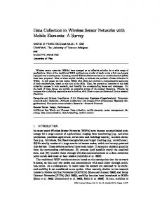
FIG. 3. Accuracy of the automatic hole-centering procedure. (A) An image (upper left) of a Quantifoil grid (R1.2/1.3) under conditions used to select positions for imaging (indicated by Xs) and three actual images recorded in an automated data collection session. (B) Quantitation of the positional accuracy of centering the hole in the field of view with (closed circles) and without (open circles) use of our automatic hole-centering algorithm. The three panels show the extent of the displacement as a net radial value (top) and along two orthogonal directions that are perpendicular (middle) and parallel (bottom) to the axis of the specimen stage.
Evaluation of the Accuracy of the Automated Procedures Figure 3A provides a graphical illustration of the effectiveness of the hole-centering algorithm by displaying representative images recorded in a typical automated data collection session. It is clear that a majority of the hole area is included in each of the recorded images. A more quantitative assessment of the accuracy of stage positioning with and without the use of the hole-centering algorithm is shown in Fig. 3B. In the absence of compensation, the mechanical “wobble” of the goniometer results in hole displacements that are greater than 0.6 m even when great care is exercised to manually center holes before they are picked in the Search mode. At 52 000⫻ magnification, this level of inaccuracy is not acceptable because it can result in the majority of the hole being moved out of the imaged area in the micrograph. Inclusion of the hole-centering algorithm results in the lowering of the positional errors
to an average displacement of 0.07 m, which corresponds to the inclusion, on average, of about 90% of the hole in the area on photographic film. Analysis of the direction of the displacements reveals that they arise predominantly from errors in positioning along, rather than perpendicular to, the long axis of the specimen stage. Figure 4 illustrates the accuracy of the automated focus-determination procedure. Figure 4A shows the intrinsic accuracy of the algorithm that we employ to calculate the deviation from focus. The plot compares the value returned by automated determination with the value manually set at the same magnification (220 000⫻) over a range of defocus values. All points on this plot fall close to the line with a slope of 1, establishing the reliability of the focusdetermination procedure. In a normal low-dose imaging session, however, a lower level of accuracy is expected because the focus is usually set at a higher magnification, while the image is recorded at a lower
AUTOMATED ELECTRON MICROSCOPY
257
and it should be possible to translate these into tests that can be automatically carried out by the microscope computer. As a starting point, we have implemented the simplest of such tests into AutoEM by incorporating an automated measurement of the optical density of each hole. Figure 5 shows the effectiveness of the program in assessing the thickness of the vitreous ice layer in each hole by plotting the optical density values measured on the CCD at low magnification before recording the image with the values experimentally determined from an image of the same region recorded on film at 52 000⫻. There is an approximately linear correlation between these two sets of values, suggesting that it is possible to select, with some reliability, for holes of the right thickness based on the optical density measured at low magnification. The range of variation in intensities for empty holes is ⬍0.8% for CCD measurements and ⬍1.2% for film measurements. This variation is well below the optical density difference (typically 5–10%) between an empty hole and one with a suitable thickness of ice. Assessment of Image Quality
FIG. 4. Accuracy of automatic focus determination and setting. (A) Correlation between the defocus value manually set at 220 000⫻ and the defocus value determined by the program, also at 220 000⫻. The solid line corresponds to a 1:1 correlation. (B) (‚) Underfocus values experimentally measured from film images recorded at 52 000⫻ and plotted against the values set manually at 220 000⫻. This plot serves a microscope-specific focus calibration curve. (F) Underfocus values measured experimentally from film images recorded at 52 000⫻ in a completely automated session and plotted against the values requested at the beginning of data acquisition through the user interface. The plots show that the automated focusing procedure is very reliable.
magnification. The extent of the change in focus between the different magnifications is different for each microscope and can sometimes be significant. Figure 4B shows a plot of the experimentally measured values from micrographs recorded (at 52 000⫻) vs the values set automatically (at 220 000⫻) in the course of automated data acquisition. The experimentally determined values are well described by a straight line with a slope of 0.81 and an offset of 0.11 m and closely correspond to the manual calibration curve recorded for the same set of magnifications. The selection of holes that are suitable for obtaining the best images is frequently considered to be subjective. However, any or all of the criteria used by an experienced operator should be quantifiable,
Figure 6A shows a digitized micrograph of an image recorded from a frozen-hydrated specimen using the automated procedure. Visual inspection suggests that it is comparable to micrographs recorded manually on our microscope (data not shown). To obtain a quantitative assessment of image quality,
FIG. 5. Assessment of the ice thickness in the holes. The plot shows measurements of the percentage reduction in the optical density of an ice-covered hole compared to those of an empty hole measured with a CCD at 2700⫻ before imaging ( x axis) and in the image recorded on photographic film at 52 000⫻ ( y axis). The different symbols represent data collected from different grid preparations.
258
ZHANG ET AL.
FIG. 6. Comparison of image quality between a manually collected data set and by AutoEM. (A) A cryoelectron micrograph of the one catalytic domain of pyruvate dehydrogenase from B. stearothermophilus taken at 52 000⫻ magnification. (B) Power spectra from 1000 molecular images collected using either manual or automated methods. One thousand images that roughly correspond to a fivefold view were selected. Both sets of micrographs were collected using identical electron optical conditions from the same grid square and in the same session at underfocus values of ⬃2.4 microns. (C) The average of each of these sets of 1000 images, after an initial round of self-alignment. The upper average is from automated data collection.
we recorded a series of micrographs by using manual and automated procedures on the same frozenhydrated grid containing molecules of the catalytic domain of pyruvate dehydrogenase. Both sets of images were recorded under identical electron optical conditions and with very closely matched underfocus values. One thousand molecular images from each set (five micrographs, ⬃200 particles each) were then analyzed with the IMAGIC-5 image processing package (van Heel et al., 1996). Figure 6B shows that the power spectrum from the images
recorded in the automated mode is at least as good, if not better, at most spatial frequencies as that obtained from images recorded manually, while Fig. 6C shows that the averaged images from each set are also closely comparable. Speed of Data Collection One of the motivations for implementing automation is to increase the throughput of data acquisition. Table I shows the times involved in the various steps involved in recording an image during a typi-
259
AUTOMATED ELECTRON MICROSCOPY
TABLE I Timing on Automation Steps
Remote Operation
Automation step
Seconds
Move to location Center a hole Measure ice thickness Switch to focus mode Center focus beam Burn ice at focus area Monitor specimen drifta Auto focus Take a film picture Center exposure beamb Burn off a holeb
1 6 5 3 4 11 9*n 26 33 15/5 40/5
Total
109
Note. The average timing in seconds for each of the steps executed by the program in an automated data collection session starts from the movement of the stage to the location of interest picked manually. The time to determine the drift rate is about 9 s for each measurement. Since the drift rate is continually measured, it takes 18 s for two measurements, 27 s for three measurements, and so on. The drift rate is usually within acceptable limits (set here to be 1 Å/s) after one or two measurements. Note that the drift measurement is only initiated about 30 s after the stage is moved to the area, providing sufficient time for the drift to be slowed down. The centering of the exposure beam is carried out every five exposures, thus contributing an average of 3 s per exposure. The recalibration of optical density of an empty hole is carried out by creating a hole with strong irradiation every five exposures, contributing an average of 8 s per exposure. The speed of execution of some of the steps, such as hole centering, drift monitoring, and automated focus determination, depends on the speed of the computer and could be improved with faster processors. a n, number of drift measurements. b Once every five exposures.
cal high-resolution imaging session (such as the one used to collect the data shown in Fig. 6). For the case in which the holes to be imaged have been selected by the user, the average time required per image is under 2 min, suggesting that it should be possible to collect about 30 images every hour. The actual number of images that could be collected, depends on the fraction of holes that are deemed suitable for recording a high-resolution image and the thermal and mechanical stability of the cold stage. An important limitation also arises from the degradation of the specimen over time due to contamination with ice, which results in a corresponding decline in the quality of the recorded images over several hours. In the fully automated mode, or the mode in which the user specifies the best grid squares, the time per image depends, of course, on the fraction of holes that are judged to be suitable for imaging. The time lost for every hole that is evaluated, but not used, is about 6 s, and the time lost for every grid square that is evaluated but not used is about 10 s.
Except for the steps involved in preparation of the specimen and insertion of the cold stage into the microscope, it should be possible, in principle, to carry out all other aspects of microscope control and data acquisition without requiring the user to be present in the immediate vicinity. We have successfully implemented remote operation of the microscope using a commercially available program, PC Anywhere, that hands over the control of the microscope computer to the remote computer and mirrors the display to the remote monitor. The use of a remote monitoring computer provides an excellent and convenient tool in situations in which the microscope is not situated in the immediate vicinity of either the operator or any interested observers controlling or monitoring data collection. Perhaps the most significant immediate value of the remote interface is the elimination of the thermal and acoustic interference generated by a human operator sitting at the microscope console during the recording of high-resolution images. DISCUSSION
In the process of three-dimensional structure determination of a molecular assembly by electron microscopy, one can think of three distinct stages: (i) specimen preparation, which encompasses the steps required to obtain purified protein and transfer it onto a specimen holder and into the electron microscope; (ii) data collection, which is the process of recording images at the required electron optical settings onto either film or a CCD camera; and (iii) image analysis and three-dimensional reconstruction, a step in which the information contained in a collection of images is processed computationally to arrive at the three-dimensional structure of the imaged object. In the most ambitious and futuristic implementation of automation, one could envision the construction of a microscope “machine” with which the interaction of the operator with the microscope would be limited to the injection of an aqueous solution of a suitable specimen into a port on the machine, with all of the remaining steps including preparation of a suitable specimen, data collection, and image analysis and reconstruction of the three-dimensional structure being totally automated. Although it appears unlikely that such an advanced level of automation will be available in the immediate future, there are no fundamental limitations that prevent individual steps in the process from being automated. The target of our present work is to achieve the first and simplest level of automation that would
260
ZHANG ET AL.
be useful both to regular and novice users of the microscope. Although many of the features in AutoEM bear a similarity to those available in the automated routines described by Carragher et al. (2000), there are some significant differences. First, AutoEM is specifically designed for the new Tecnai series of microscopes, while the programs described by Carragher et al. (2000) are specifically designed for the CM series of microscopes previously manufactured by FEI/Philips. Second, AutoEM can be implemented on any Tecnai microscope without additional computer requirements or changes in microscope hardware. Third, the algorithms for recording high-resolution images are completely independent of the mechanical properties of the particular microscope and specimen stage used, and they therefore do not require specialized calibration, as described for the CM series of microscopes (Pulokas et al., 1999). Finally, because of the very simplified set of criteria used for evaluating grid squares and holes suitable for imaging and the fast-focus determination procedure, the set-up time before data collection begins is minimal. Once a satisfactory vacuum has been achieved in the column, the set-up time to invoke a semiautomated data collection session is about 10 –15 min, while the set-up time to invoke a fully automated data collection is about 5 min. The level of automation embodied in AutoEM has been useful in our laboratory both for experienced electron microscopists who choose to manually select regions to be imaged and for users who choose to have all decisions about data collection be carried out automatically. At the present level of implementation, the automated collection of many hundreds of high-quality images a day is possible, but we are not yet at a stage at which we can take full advantage of this capability. One limitation arises from the fact that the cold stages we currently use maintain the specimen at liquid nitrogen temperatures for a duration of 6 h in the best case. Thus, a 24-h data collection would require four to five refills of the dewar. Installation of an automated dewar-filling robot may circumvent this problem, but may not be the best solution to the problem. Cold stages with dewars that have greater capacity would be an alternative solution, but these are not yet available for the side-entry cold stages marketed currently. While the capacity of the dewar is potentially a limitation for collection of large numbers of images, it is not the most significant issue for our present purposes. One technical limitation to the collection of large data sets of images arises from the contamination of the cold specimen from the deposition of ice originating from water molecules in the microscope column (Henderson, 1992). The vacuum that
is realized in the columns of many present-generation microscopes is sufficiently poor to result in a substantial degradation of image quality after the specimen is exposed to the column for a few hours. Our experience with the Tecnai 12 microscope is that there is significant degradation in image quality about 5– 6 h after the specimen is inserted into the microscope. A further limitation arises from the fact that images recorded digitally with the best available CCD cameras are still inferior to those recorded on photographic film because of the decay of the CCD modulation transfer function at high spatial frequencies (Downing and Hendrickson, 1999; Sherman et al., 1996). Thus, to obtain the highest possible resolutions in molecular microscopy, photographic film continues to be the recording medium of choice. Only 56 films are presently accommodated in a Tecnai microscope cassette, requiring the presence of the operator every 2–3 h to exchange the cassette in a typical automated data collection session. Since no refilling of liquid nitrogen is required over this short time period, equipment for automated refilling of the cold stage is unnecessary for this mode of data collection. With the continuing improvements in CCD detectors, it will not be long before the quality of digitally recorded images becomes comparable to those recorded on photographic film (Faruqi and Subramaniam, 2000). High-throughput digital data collection will then become the norm, rather than the exception. Future developments in AutoEM will be aimed at increasing the ease of processing digitally collected or digitized images, introducing more sophisticated criteria for selecting regions to be imaged, and providing the remote user with improved, instantaneous, and quantitative measures of the quality of the data that are being collected. This work was supported by funds from the intramural program at the National Cancer Institute. We thank Drs. Richard Perham and Gonzalo Domingo for the gift of the purified preparation of the catalytic domain of pyruvate dehydrogenase from B. stearothermophilus. We thank Drs. M. Kessel, D. Shi, T. Hirai, J. Heymann, and M. Borgnia for helpful discussions. REFERENCES Allen, M. D., and Perham, R. N. (1997) The catalytic domain of dihydrolipoyl acetyltransferase from the pyruvate dehydrogenase multienzyme complex of Bacillus stearothermophilus. Expression, purification and reversible denaturation. FEBS Lett. 413, 339 –343. Carragher, B., Kisseberth, N., Kriegman, D., Milligan, R. A., Potter, C. S., Pulokas, J., and Reilein, A. (2000) Leginon: An automated system for acquisition of images from vitreous ice specimens. J. Struct. Biol. 132, 33– 45. Downing, K. H., and Hendrickson, F. M. (1999) Performance of a
AUTOMATED ELECTRON MICROSCOPY 2k CCD camera designed for electron crystallography at 400 kV. Ultramicroscopy 75, 215–233. Faruqi, A. R., and Subramaniam, S. (2000) CCD detectors in high-resolution biological electron microscopy. Q. Rev. Biophys. 33, 1–27. Henderson, R. (1992) Image contrast in high-resolution electron microscopy of biological macromolecules: TMV in ice. Ultramicroscopy 46, 1–18. Koster, A. J., Chen, H., Sedat, J. W., and Agard, D. A. (1992) Automated microscopy for electron tomography. Ultramicroscopy 46, 207–227. Lepault, J., Booy, F. P., and Dubochet, J. (1983) Electron microscopy of frozen biological suspensions. J. Microsc. 129(Pt. 1), 89 –102. McDowall, A. W., Chang, J. J., Freeman, R., Lepault, J., Walter,
261
C. A., and Dubochet, J. (1983) Electron microscopy of frozen hydrated sections of vitreous ice and vitrified biological samples. J. Microsc. 131, 1–9. Oostergetel, G. T., Keegstra, W., and Brisson, A. (1998) Automation of specimen selection and data acquisition for protein electron crystallography. Ultramicroscopy 74, 47–59. Pulokas, J., Green, C., Kisseberth, N., Potter, C. S., and Carragher, B. (1999) Improving the positional accuracy of the goniometer on the Philips CM series TEM. J. Struct. Biol. 128, 250 –256. Sherman, M. B., Brink, J., and Chiu, W. (1996) Performance of a slow-scan CCD camera for macromolecular imaging in a 400 kV electron cryomicroscope. Micron 27, 129 –139. van Heel, M., Harauz, G., and Orlova, E. V. (1996) A new generation of the IMAGIC image processing system. J. Struct. Biol. 116, 17–24.