The goal of performance regression testing is to check for performance ..... In large software systems, e.g., Google search engine or large web server farms, there ...
Automated Detection of Performance Regressions Using Statistical Process Control Techniques Thanh H. D. Nguyen, Bram Adams, Zhen Ming Jiang, Ahmed E. Hassan
Mohamed Nasser, Parminder Flora Performance Engineering Research In Motion (RIM) Waterloo, Ontario, Canada
Software Analysis and Intelligence Lab (SAIL) School of Computing, Queen’s University Kingston, Ontario, Canada {thanhnguyen,bram,zmjiang,ahmed}@cs.queensu.ca
ABSTRACT
hour of a typical test run can produce millions of samples for hundreds of performance counters, which require a large amount of time to analyze. Unfortunately, performance regression testing is usually performed at the end of the development cycle, right before a tight release deadline; allowing very little time for performance engineers to conduct and analyze the tests.
The goal of performance regression testing is to check for performance regressions in a new version of a software system. Performance regression testing is an important phase in the software development process. Performance regression testing is very time consuming yet there is usually little time assigned for it. A typical test run would output thousands of performance counters. Testers usually have to manually inspect these counters to identify performance regressions. In this paper, we propose an approach to analyze performance counters across test runs using a statistical process control technique called control charts. We evaluate our approach using historical data of a large software team as well as an open-source software project. The results show that our approach can accurately identify performance regressions in both software systems. Feedback from practitioners is very promising due to the simplicity and ease of explanation of the results.
1.
Control charts is a statistical control technique that has been widely used in manufacturing processes [16] where quality control is essential. A manufacturing process has inputs, i.e., raw materials, and output, i.e., products. Control charts can detect deviations in the output due to variations in the process or inputs across different manufacturing runs. If there is a high deviation, an operator is alerted.
INTRODUCTION
Performance regression testing is an important task in the software engineering process. The main goal of performance regression testing is to detect performance regressions. A performance regression means that a new version of a software system has worse performance than prior versions. After a development iteration of bug fixes and new features, code changes might degrade the software’s performance. Hence, performance engineers must perform regression tests to make sure that the software still performs as good as previous versions. Performance regression testing is very important to large software systems where a large number of field problems are performance related [19]. Performance regression testing is very time consuming yet there is usually little time allocated for it. A typical test run puts the software through a field-like load for an extended period of time, during which performance counters are collected. The number of counters is usually very large. One
A software system is similar to a manufacturing process. There are data inputs, e.g., the load inputs, and data outputs, e.g., the performance counters. When performance regressions occur, the output performance counters deviate. A control chart can potentially be applied to compare performance regression tests where the process inputs are the load, e.g., page requests on a web server, and the process outputs are performance counters, e.g., CPU utilization or disk IO activities. Unfortunately, control charts have two assumptions about the data that are hard to meet in a performance regression test. First, control charts assume that the outputs, i.e., performance counters, have a uni-modal normal distribution, since deviations are defined from the mean of such a distribution. Second, control charts assume that the load inputs do not vary across runs. If the inputs are different, the counters would fluctuate according to the inputs. Since both assumptions do not hold for performance load tests, it seems that control charts cannot be applied to this domain as is. In this paper, we propose an approach that customizes control charts to automatically detect performance regressions. It addresses the two issues with the assumptions mentioned above. To evaluate our approach, we conduct a case study on a large enterprise software system and an open-source software system. Feedback from practitioners indicates that the simplicity of our approach is a very important factor, which encourages adoption because it is easy to communicate the results to others. The contributions of this paper are:
1
• We propose an approach based on control charts to identify performance regressions.
limit. The LCL and the UCL can be defined in several ways. A common choice is three standard deviations from the CL. Another choice would be the 1th , 5th , or 10th percentiles for the LCL and 90th , 95th , or 99th percentiles for the UCL. For example: there are eleven response time readings of 3, 4, 5, 6, 7, 8, 9, 10, 11, 12, and 13 milliseconds in the baseline set. If we use the 10th and the 90th percentile as control limits, the LCL, CL, and UCL would be 4, 8, and 12 respectively.
• We derive effective solutions to satisfy the two assumptions of control charts about non-varying load and normality of the performance counters. • We show that our approach can automatically identify performance regressions by evaluating its accuracy on a large enterprise system and an open-source software system.
The target dataset is then scored against the control limits of the baseline dataset. In Figure 1(a) and 1(b), the target data are the crosses. Those would be the response time of the current operating periods, e.g., the current hour or day.
The paper is organized as follows. In the next section, we introduce control charts. Section 3 provides the background on performance regression testing and the challenges in practice. Section 4 describes our control charts based approach, which addresses the challenges. In Section 5, we present the two case studies, which evaluate our approach. Section 6 summarizes the related work and the feedback from practitioners on our approach. We conclude in Section 7.
The result of an analysis using control charts is the violation ratio. The violation ratio is the percentage of the target dataset that is outside the control limits. For example, if the LCL and the UCL is 4 and 12 respectively, and there are ten readings of 4, 2, 6, 2, 7, 9, 11, 13, 8, and 6, then the violation ratio is 30% (3/10). The violation ratio represents the degree to which the current operation is out-of-control. A threshold is chosen by the operator to indicate when an alert should be raised. A suitable threshold must be greater than the normally expected violation ratio. For example, if we choose the 10th and the 90th percentile as control limits, the expected violation ratio is 20%, because that is the violation ratio when scoring the baseline dataset against the control chart built using itself. So, the operator probably wants to set a threshold of 25% or 30%.
2. CONTROL CHARTS 2.1 What Are Control Charts? Control charts were first introduced by Shewhart [16] at Bell Labs, formerly known as Western Electric, in the early 1920s. The goal of control charts is to automatically determine if a deviation in a process is due to common causes, e.g., input fluctuation, or due to special causes, e.g., defects. Control charts were originally used to monitor deviation on telephone switches.
2.3
Assumptions of Control Charts
There are two basic assumptions of control charts: Control charts have since become a common tool in statistical quality control. Control charts are commonly used to detect problems in manufacturing processes where raw materials are inputs and the completed products are outputs. We note that, despite the name, control charts is not just a visualization technique. It is a statistical technique that outputs a measurement index called violation ratio.
Non-varying process input. Process output usually fluctuates with the process input. If the process input rate increases, the violation ratio will increase and an alert will be raised independent of how the system reacts to the fluctuation input. Such alert would be a false positive because it does not correspond to a problem. So, the first condition for applying control charts is the stability of the process input.
Figure 1(a) and 1(b) show two example control charts. The x-axis represents time, e.g., minutes. The y-axis is the process output data. For this example, we are monitoring the response rate of a web server. The two solid lines are the Upper Control Limits (UCL) and Lower Control Limit (LCL) in between which the dashed line in the middle is the Centre Line (CL). Figure 1(a) is an example where a process output is within its control limits. This should be the normal operation of the web server. Figure 1(b), on the other hand, is an example where a process output is out-of-control. In this case, operators should be alerted for further investigation.
2.2
Normality of process output. Process output usually has a linear relationship with the process input. This linear relation leads to a normal distribution of the process output which is the main underlying statistical foundation of control charts. However, some manufacture processes take multiple types of input, each of which individually still output a normal distribution. However, the combination of these inputs would have a multi-modal distribution, which is impossible to compare using control charts. In the following section, we explain in details why these two assumptions are hard to meet in performance regression testing. We will give examples for each condition and propose solutions to adapt the performance counters such that we can apply control charts to detect performance regressions.
Construction of Control Charts
A control chart is typically built using two datasets: a baseline dataset and a target dataset. The baseline dataset is used to create the control limits, i.e., LCL, CL, and UCL. In the example of Figure 1(a) and 1(b), the baseline set would be the response time of the web server in the previous hour, previous day, or any past operation periods. The CL is the median of all samples in the baseline dataset during a particular period. The LCL is the lower limit of the normal behaviour range. The UCL is the upper
3.
PERFORMANCE REGRESSION TESTING
Performance regression test is a kind of load test that aims to detect performance regressions in the new version of a software system. A performance regression means that the new version uses more resources or has less throughput than prior versions. We note the difference between performance 2
x
x x x x x
x
x x x x x x x xx x x xx x
x
Response time
Response time
x
Baseline LCL,UCL Baseline CL x Target
x x x x x xxx xx x x x x x x x x x x x x x x x x x x xxx x
Baseline LCL,UCL Baseline CL x Target
x x x x x x x x xx x x x x xx xx x x x x x x x x xx x x xx x x x x x x xx x xx x xx xx xx x x x
Time
Time
(a) Normal operation
(b) Out-of-control
Figure 1: Example of a control chart, which detects deviation in process output. Apply standard load on an existing software version e.g. v1.0
Baseline perf. counters e.g. % CPU usage
Apply the same the load on a new software version e.g. v1.1
Target perf. counters e.g. % CPU usage
Detect performance regression
Regression Report e.g. pass or failed
Figure 2: Conceptual diagram of performance regression testing. • Disk IO: the amount of disk input and output.
regression testing and stress testing (which is not the focus of this paper). The goal of stress testing is to benchmark the maximum load a software system can handle. The goal of a performance regression testing, on the other hand, is to determine if there is a performance regression between software versions at a normal field-like load. Figure 2 shows a conceptual diagram of a performance regression testing process which is very similar to other regression testing (e.g, functional regression testing).
Detect performance regressions. After the tests are done, the test engineers have to analyze the performance counters. They compare the counters of the new version with the existing version. The runs/counters of the existing version are called the baseline runs/counters. The runs/counters of the new version are called the target runs/counters. If the target counters are similar to the baseline counters, the test will pass, i.e., there is no performance regression. Otherwise, the test engineers will alert the developers about the potential of performance regression in the new version. For example, if the baseline run uses 40% of CPU on average and the target run uses 39% of CPU on average, the new version should be acceptable. However, if the target run uses 55% of CPU on average, there is likely a performance problem with the new version.
Apply the load. Both the existing version and the new version are put through the same load input. The load input is usually called a load profile which describes the expected workload of the system once it is operational in the field [1]. A load profile consists of the use case scenarios and the rate of these scenarios. For example, a commercial website should process 100 page requests/sec. So the test engineers would use a load generator to create 100 pages requests/sec which are directed to the web server under test. This rate is maintained for several hours or even a few days. To mimic real life, the rate is applied using a randomizer instead of applying it in a constant fashion.
3.1
Challenges in Detecting Performance Regressions
There is already good commercial support for executing performance regression test and recording performance counters. HP has the LoadRunner software [9], which can automatically simulate the work load of many network protocols. Microsoft also has a load test tool, which can simulate load on web sites or web services. The tool is offered as part of the Visual Studio suite [14]. On the other hand, detecting performance regression is usually done manually.
During the test, the application is monitored to record the execution logs and performance counters data. In our case, we are only interested in performance counters. A load test typically collects four main types of performance counters: • CPU utilization: the percentage of utilized CPU per thread (in percentage).
Challenge 1: Many performance counters to analyze.
• Memory utilization: the used memory (in megabytes). • Network IO: the amount of network transfer (in and out - in megabytes).
In large software systems, e.g., Google search engine or large web server farms, there are many components across several 3
machines. The total number of counters are in the thousands with each counter being sampled at a high rate leading to millions of data samples to analyze. Comparing the counters to find performance regressions is very time consuming.
counters in all the baseline runs, i.e., the runs of prior versions, to determine the control limits for the control chart. Then, we score the target run using those limits. The resulted violation ratio is an indicator of performance regressions in the new software version. If the violation ratio is high, the chance of a regression is high as well. If the violation ratio is low, the chance of a regression is low.
Challenge 2: Inconsistent performance counters across test runs. A big assumption in performance regression testing, as conceptualized in Figure 2, is that the performance counters will be the same if the software does not change. Thus, if the baseline run uses X% of CPU and target run also uses X%, then there is no change in the performance, i.e., there are no performance regressions. On the opposite side, if the target run uses >X% of CPU, then there is likely a performance regression. The assumption here is that X% is a fixed number.
An approach based on control charts would address the two challenges of performance regression testing. Control charts provide an automated and efficient way to use previous baseline runs to compare against a new test run without having to perform more baseline runs (i.e., with minimal human intervention). However, to apply control charts to detect performance regressions, we have to satisfy the two assumptions of control charts explained in Section 2: non-varying process input and normality of the output. Unfortunately, these two assumptions are difficult to meet if we use the performance counters as is. Hence we propose two preprocessing steps on the counter data before constructing the control chart. These steps are represented as the Scale and Filter processing boxes in Figure 3). In the next two subsections, we describe in detail each of the proposed solutions and evaluate their effectiveness.
In a large software system, the output performance counters might be different due to the nondeterministic nature of the system. For example, a web server would cache the recently accessed web pages to improve performance. If there is a high burst of page requests at the beginning of a test run, the performance of the rest of the run will be remarkably better than if the high burst happens at the end of the run, because the cache would be filled faster in the former case. Hence, five different baseline runs can yield 57%, 65%, 62%, 56%, and 60% of CPU utilization. Although all the runs average at about 60%, it is not clear if 60% should be the baseline to compare against when a new version of the software is tested. If the new version’s run yields a 65% CPU utilization, can we be certain that there is a performance regression? After all, there is one baseline run that uses 65% CPU.
4.1
To eliminate uncertainty, every time a new test run is performed, the testers usually have to rerun the old version test right after so they can compare between the two runs. The extra run is very time consuming.
4.
A CONTROL CHARTS BASED APPROACH TO DETECT PERFORMANCE REGRESSIONS
A good approach to detect performance regressions should address the two aforementioned challenges from the previous section.
Satisfying the Non-Varying Input Assumption
In performance regression testing (Figure 2), the same load is applied to both the baseline and target version. For example if the load profile specifies a rate of 5,000 requests per hour, the load generator will aim for 5,000 requests per hour in total using a randomizer. The randomization of the load is essential to trigger possible race conditions and to ensure a realistic test run. However, the randomization leads to varying inputs throughout the different time periods of a test run. The impact of randomization on the input load and the output counters increases as the system becomes more complex with many subcomponents having their own processing threads and timers. Even in the Dell DVD Store system [5] (see Section 5), which is a relatively small and simple system, the load driver employs a randomizer. This randomizer makes it impossible to get two similar test runs with the same effective load input. If the input load are different between runs, it is difficult to identify performance regressions since the difference in the counters can be caused by the different in the input load instead of performance related changes in the code. Figure 5 shows a performance counter of two different runs coming from two successive versions of a software system (see Section 5 for more details). We divide the runs into eight equal periods of time (x-axis). The y-axis shows the median of the performance counter during that period. The red line with round points is the baseline, which is from an earlier build. The blue line with triangular points is the target, which is from the new build. According to documentation, the fixes between the two builds should not affect the performance of the system. Hence, the performance counters should be very similar. Yet, it turns out that they are different because of the variation in the effective input load due to randomization of the load. The smallest difference is 2% in the eighth
Trubin et al. [18] proposed the use of control charts for infield monitoring of software systems where performance counters fluctuate according to the input load. Control charts can automatically learn if the deviation is out of a control limit, at which time, the operator can be alerted. The use of control charts for monitoring inspires us to explore them for the study of performance counters in performance regression tests. A control chart from the counters of previous test runs, may be able to detect “out of control” behaviours, i.e., deviations, in the new test run. The difficulty though is that we want to detect deviations of the process, i.e., the software system, not the deviations of the input, i.e., the load. Figure 3 shows a conceptual overview of our proposed control charts based approach. For each counter, we use the 4
Scale
Filter
Baseline test 1 Counter 1
Repository of load test results
Create Control Chart
●
Performance Counter
Target test Counter 1
Run new target test
● ●
●
1
2
●
●
●
●
●
3
4
5
6
Baseline LCL Baseline CL Baseline UCL Target 7
8
Time periods
Scale
Filter
Baseline test 2 Counter 1
Violation ratio
Figure 3: Outline of our approach to detect performance regression.
4.1.2
period. The highest difference is 30% in the first period. On average, the difference is about 20%. The actual load inputs are about 14% different between the two runs.
4.1.1
Proposed Solution
Our proposal is to scale the performance counter according to the load. Under normal load and for well designed systems, we can expect that performance counters are proportionally linear to the load intensity. The higher the load, the higher the performance counters are. Thus, the relationship between counter values and the input load can be described with the following linear equation:
c=α∗l+β
We run a set of controlled test runs to build the linear model as in (1). The control runs use the same stable version. We pick a different target load for each test. For example, if the first three runs have actual loads of 1,000, 1,200, and 1,000, we will aim for a load of 1,200 for the fourth run. This choice ensures that we have enough data samples for each load level, i.e., two runs with 1,000 and two runs with 1,200 in this example.
(1)
For each test run, we extract the total amount of load l and the mean performance counter c for each period of the runs. Then we train a linear model to determine α and β using part of the data. Then we can test the accuracy of the model using the rest of the data. This technique is used commonly to evaluate linear models. A common ratio for train and testing data is 2:1. We randomly sample two-thirds of the periods to train the linear model. Then we use the remaining one-third to test the model. We repeat this process 50 times to eliminate possible sampling bias.
In this equation, c is the average value of the performance counter samples in a particular period of a run. l is the actual input load in that period. α and β are the coefficients of the linear model. To minimize the effect of load differences on the counters, we derive the following technique to scale each counter of the target run: • We collect the counter samples (cb ) and corresponding loads (lb ) in the baseline runs. For example, in third minute the CPU utilization is 30% when the load is 4,000 requests per minute. In the next minute, the load increases to 4,100 so the CPU utilization increases to 32%.
Results. Figure 4 shows the result of our evaluation. The graph on the left is the box plot of the Spearman correlation between the predicted and the actual counter values. If the Spearman correlation nears zero, the model is a bad one. If the Spearman correlation nears one, then the model fits well. As we can see, all 50 random splits yield very high correlations. The graph on the right is the box plot of the mean error between the predicted and the actual counter values. As we can see, the errors, which are less than 2% in most cases, are very small. These results show that the linear model used to scale the performance counters based on the actual load is very accurate.
• We determine α and β by fitting counter samples, e.g. the CPU utilization, and the corresponding load, e.g. the number of requests per second, into the linear model: cb = α ∗ lb + β as in (1). The baseline runs usually have thousands of samples, which is enough to fit the linear model. • Using the fitted α and β, we can then scale the corresponding counter of the target run (ct ) using the corresponding load value (lt ) as in (2).
ct = cb ∗
α ∗ lt + β α ∗ lb + β
Evaluation
Evaluation Approach. The accuracy of the scaling technique depends on the accuracy of the linear model in (1). To evaluate the accuracy of the linear model, we need to use the test runs of a software system. Hence, we evaluate the accuracy on an industrial software system (see Section 5 for more information).
Example. Figure 6 shows the performance counters of the two runs in Figure 5 after our scaling. The counters of the two tests are now very similar. As we can see, after scaling, the target runs fluctuate closer to the baseline test. The difference between the two runs is about 9% (between 2% to 15%) after scaling compared to 20% (between 2% to 30%) without scaling (Figure 5).
(2)
5
Error
1.0
Correlation
●
●
●
−2
0
●
●
●
1 2
●
−4
CPU utilization
0.6 0.4 0.2
Spearman's rho
0.8
Performance Counter
2
● ●
1
2
3
4
5
6
7
8
−6
0.0
Time period
Figure 5: The performance counters of two test runs. The difference in performance is not a performance regression since both runs are of very similar builds. The difference (20% average) is due to differences in the actual load.
Figure 4: The accuracy of the linear model in (1). Left: The Spearman correlations between the predicted and actual performance counter values of 50 random splits. Right: The errors between the predict and actual value in percentage.
4.2
Satisfying the Normality of Output Assumption
Process output is usually proportional to the input. So the counter samples’ distribution should be a uni-modal normal distribution (unless the load is pushed to the maximum, as in stress testing, the counter distribution will skew to the right). However, the assumption here is that there is only one kind of effective load input. If there are many kinds of input, the distribution of counters would be multi-modal as we explained in Section 2.3. Figure 9 shows the normal QQ plot of a performance counter of a software under test (the Enterprise system in Section 5). If the counter is uni-modal, its samples should form a diagonal straight line. As we can see, the upper part of the data fluctuates around a diagonal straight line. However, the lower end does not. Unfortunately, the data points at the lower end are not outliers; they appear in all test runs of the software. As such, the overall distribution is not uni-modal. A Shapiro-Wilk normality test on the data confirms that with p < 0.05.
When the system is under a load, the performance counters respond to the according load in a normal distribution. However, in between periods of high load, the performance counter is zero since there is no load input. The first point on the density plot for both runs is about 4%. Hence, the performance counter is at zero for about 4% of the time during both test runs. The target run spent 5% of its time at semi-idle state (the second point from the left on the red curve). We discover that, when there is no load, the system performs book keeping tasks. These tasks require only small amounts of resources. We can consider these tasks as a different kind a load input. These secondary tasks create a second peak in the distribution curve, which explains the long tail in the QQ plot of Figure 9. Unfortunately, this is a common behaviour. For example, on a web server, a web page would contain images. When a web page is requested by the client, the web server has to process and serve the page itself and the attached images. The CPU cycles required to process an image are almost minimal. Web pages, on the other hand, require much more processing since there might be server side scripts on them. Thus the distribution of the CPU utilization would be a bi-modal distribution. The main peak would correspond to processing the web pages. The secondary peak would correspond to processing the images. In the software system we study, only 16% of the studied test runs are uni-modal. We confirm that these runs are, in fact, normal as confirmed by Shapiro-Wilk tests (p > 0.05). The majority of the runs, which is about 84%, have a bi-modal distribution similar to that of the target run in Figure 7. In the bi-modal runs, the left peak corresponds to the idle-time spent on book-keeping tasks. The right peak corresponds to the actual task of handling the load. The relative scale of the two peaks depends on how fast the hardware is. The faster the hardware, the more time the system idles, i.e.,
Figure 7 shows a density plot of a performance counter of two test runs of the same software under test. These two runs come from two successive versions. The green line with round points is the baseline run, which is based on an older version. The red line with triangles is the target, which is from a new version. As we can see in the graph, the distribution of the performance counters resembles a normal distribution. However, the left tail of the distribution always stays up instead of decreasing to zero. 6
40 35 ● ●
25
●
●
10
Performance Counter
Density %
●
20
●
●
15
●
●
30
●
●
●
5 0 2
3
4
5
6
7
20 15
●
Baseline Target LCL,UCL
●
5
●
●
●
●
●
0
●
●
●
●
●
●
●
●
●
An alternative solution is to increase the load as the server hardware becomes more powerful. The increased load will make sure that the system spends less time idling and more time processing the load, thus, removing the left peak. However, artificially increase the load for the sake of normality defeats the purpose of performance regression testing and compromises the ability to compare new tests to old tests. ●
4.2.2 Performance counter
Evaluation
Evaluation Approach. To evaluate the effectiveness of our filtering technique, we pick three major versions of the software system (the Enterprise system in Section 5) that we are most familiar with. For each run of the three versions, we generate a QQ plot and run the Shapiro-Wilk normality test to determine if the runs’ performance counters are normal. Then, we apply our filtering technique and check for normality again.
Figure 7: Density plot of two test runs.
the left peak will be higher. The slower the hardware, the less time the system has to idle because it has to use more resource to process the load. The right peak will be higher and the left peak might not be there. The two runs shown in Figure 7 are on relatively standard equipment. Figure 8 shows another two test runs that are performed on better hardware configurations. As we can see, the left peaks in the density plots are more prominent in the runs with better hardware.
4.2.1
●
To implement the filtering solution, we derive a simple algorithm to detect the local minima, i.e., the lowest point between the two peaks of a bi-modal distribution. Then, we simply remove the data points on the left of the local minima. The algorithm is similar to a high pass filter in an audio system. For example, after the filtering is applied, the first three points on the target run’s density plot in Figure 7 (the red line with triangles) would become zeros.
●
●
●
Figure 8: Density plot of another two different test runs. These two runs are on a better hardware system so the left peak is much higher than the two runs in Figure 7.
10
Density %
●
●
●
8
Figure 6: The scaled performance counters of two test runs in Figure 5. We scale the performance counter according to the load to minimize the effect of load differences between test runs. The average difference between the two runs is only 9% as compared to 20% before scaling.
●
●
Performance counter
Time period
●
●
●
1 2
●
1
Baseline Target LCL,UCL
●
Results. We first manually inspect the density plots of each run in the three versions. About 88% of the runs have a bi-modal distribution. About 66% do not have a normal distribution, i.e., the Shapiro-Wilk tests on these runs return p < 0.05. If the left peak is small enough, it will pass the normality test. After filtering, 91% of the non-normal runs become normal. We believe this demonstrates the effectiveness of our filtering solution.
Proposed Solution
Our proposed solution is to filter out the counters’ samples that correspond to the secondary task. The solution works because performance regression testing is interested in the performance of the system when it is under load, i.e., when performance counters record relatively high values. Small deviations are of no interest.
Example. Figure 10 shows the QQ plot of the same data as in Figure 9 after our filtering solution. As we can see, the data points are clustered more around the diagonal line. This means that the distribution is more normal. We perform the Shapiro-Wilk normality test on the data to confirm. 7
●
●
●
12
12
●
●
●
●
●
10 4
10 8 6
Sample Quantiles
8 6
Sample Quantiles
● ●● ●
4
● ● ●● ●
2
● ● ● ●●● ● ● ●●
●
−2
−1
0
1
2
Case Study Design
To measure the accuracy of our approach: a) We need to pick a software system with a repository of good and bad tests. b) For each test in the repository we use the rest of the tests in the repository as baseline tests. We build a control chart using these tests to create the control limits. These control limits are, then, used to score the picked test. c) We measure the violation ratio and determine whether a test has passed or failed. d) We measure the precision and recall of our approach using the following formulas by comparing against the correct classification of a test:
|classif ied bad runs ∩ actual bad runs| |actual bad runs|
1
2
Table 1: Properties of the two case studies Factor Enterprise DS2 Functionality Telecommu- Enication Commerce Vendor’s business model Commercial Open-source Size Large Small Complexity Complex Simple Known counter to ana- Yes, use No, use all lyze CPU Determining kinds of Unknown Known performance Source of performance re- Real Injection gression
In this section, we describe the two case studies that we conduct to evaluate the effectiveness of our control charts based approach for detecting performance regressions.
recall =
0
Figure 10: Normal QQ plot of the performance counters after our filtering process. The data is the same as in the QQ plot of Figure 9. After we remove the data that corresponds to the idle-time tasks, the distribution becomes normal.
CASE STUDIES
|classif ied bad runs ∩ actual bad runs| |classif ied bad runs|
−1
Theoretical Quantiles
The test confirms that the data is normal (p > 0.05). We can now use the counter data to build a control chart.
precision =
●
−2
Figure 9: Normal QQ plot of CPU utilization counters. We show only 100 random samples of CPU utilization from the run to improve readability.
5.1
●● ● ● ●● ●● ● ●●● ● ●●●● ●●●● ● ●●●●● ●●● ●●● ● ● ●●●● ●●●● ●●●● ●●●● ●● ● ●●●●● ● ● ●● ●● ●●●●● ●●●● ●●● ● ●● ●●● ●● ●●
●
Theoretical Quantiles
5.
●
●
●● ●●● ●● ● ● ●● ●● ● ● ● ●● ●●●●● ●●● ● ●● ●● ● ●●●● ●●●●●● ●●●● ●●●●● ●●● ●●●● ●● ● ● ●●●● ●●●●●● ●●●● ●●●
●
●
●
●
sion tests is to keep the CPU utilization low because the engineers already know that CPU is the most performance sensitive resource. On the other hand, the DS2 system is new. We do not know much about its performance characteristic. Thus, we have to analyze all performance counters.
(3)
What kind of performance regression problems can we detect? In the Enterprise system, the testers’ classification of the test results is available. Hence, we can calculate the precision and recall of our approach on real-life performance problems. However, we do not know what kind of performance regression problems our approach can detect since we cannot access the code. On the other hand, we have the code for DS2. Thus, we inject performance problems, which are well known in practice [8], into the code of DS2 and run our own test runs.
(4)
There are three criteria that we considered in picking the case studies. We pick two case studies that fit these criteria. The first case study is a large and complex enterprise software system (denoted as Enterprise system). The second one is a small and simple open-source software (denoted as DS2). Table 1 shows a summary of the differences between the two case studies.
What is the threshold for the violation ratio? For the enterprise system, we study the impact of different violation ratios. For the DS2 system, we show an automated technique to determine the threshold. The technique can be used for the enterprise system as well.
Which performance counters should be analyzed? In the Enterprise system, the focus of the performance regres8
●
80
0.8
●
1
100
●
Table 2: Dell DVD store configuration Property Value Database size Medium (1GB) Number of threads 50 Ramp rate 25 Warm up time 1 minutes Run duration 60 minutes Customer think time 0 seconds Percentage of new customers 20% Average number of searches per order 3 Average number of items returned in 5 each search Average number of items purchased per 5 order
●
0.4 0.6 F−measure
●
●
0.2
●
20
Recall Precision 40 60
● ●
0
●
Precision Recall F−measure
Threshold
When the threshold increases, our classifier marks more runs as bad, in which case the precision (blue with circles) will increase but the recall (red with triangles) will decrease. The f-measure (brown with pluses) is maximized when both the precision and recall are at the optimum balance. The higher the f-measure, the better the accuracy. The f-measure is highest when the precision is 75% precision and the recall is 100%.
Figure 11: The accuracy of our automated approach compared the engineers’ evaluation in the Enterprise case study.
5.2
Case study 1: Enterprise system
The system is a typical multiple-tier server client architecture. The performance engineers perform performance regression tests at the end of each development iteration. The tests that we use in this study exercise load on multiple subsystems residing on different servers. The behaviour of the subsystems and the hardware servers is recorded during the test run. The test engineers then analyze the performance counters. After the runs are analyzed, they are saved to a repository so test engineers can compare future test runs with these runs.
�
�
Case study 2: Dell DVD store
The Dell DVD store (DS2) is an open-source three-tier web application [5] that simulates an electronic commerce system. DS2 is typically used to benchmark new hardware system installations. We inject performance regressions into the DS2 code. Using the original code, we can produce good runs. Using the injected code, we can produce bad runs. We set up DS2 in a lab environment and perform our own tests. The lab setup includes three Pentium III servers running Windows XP and Windows 2008 with 512MB of RAM. The first machine is the MySQL 5.5 database server [15], the second machine the Apache Tomcat web application server [17]. The third machine is used to run the load driver. All test runs use the same configuration as in Table 2. During each run, all performance counters associated with the Apache Tomcat and MySQL database processes are recorded.
Evaluation Approach
We first establish the baseline for our comparison. We do this with the help of the engineers. For each test run, we ask the engineers to determine if the run contains performance regressions, i.e., it is a bad run, or not, i.e., it is a good run. We used the engineers’ evaluation instead of ours because we lack domain knowledge and may be biased. We compare our classifications with the engineers’ classification and report the accuracy. However, we need to decide on a threshold, t, such that if the violation ratio Vx > t, run x is marked as bad. For this study we explore a range of values for t, to understand the sensitivity of our approach to the choice of t.
5.2.2
Our approach can identify test runs having performance regressions with 75% precision and 100% recall in a real software project.
5.3
We pick a few versions of the software that we are most familiar with for our case study. There are about 110 runs in total. These runs include past passed runs without performance regressions and failed runs with performance regressions. We note that we also used this dataset to evaluate the effectiveness of the scale and the filter processing in Section 4.1 and Section 4.2.
5.2.1
�
�
5.3.1
Evaluation Approach
Create data. We perform the baseline runs with the original code from Dell. We note, though, that one particular database connection was not closed properly in the original code. So we fix this bug before running the tests. Then, we perform the bad runs with injected problems. In each of these bad runs, we modify the JSP code to simulate common inefficient programming mistakes that are committed by junior developers [8]. Table 3 shows the scenarios we simulate. Each of these scenarios would cause a performance regression in a test run.
Results
Figure 11 shows the precision, recall, and F-measure of our approach. The threshold increases from left to right. We hide the actual threshold values for confidentiality reasons. 9
Table 3: Common inefficient programming scenarios Scenario Good Bad Query Limit the number of Get everything then limit rows returned by the filter on the web database to what will server be displayed System Remove unnecessary Leave debug log print debug log printouts printouts in the code DB con- Reuse database con- Create new connecnection nections when possi- tions for every query ble Key in- Create database Forget to create index dex index for frequently for frequently used used queries queries Text in- Create full-text index Forget to create fulldex for text columns text index for text columns
Table 4: Target run: System print, Baseline: Good runs 1, 2, 3, 4, and 5 Counter Threshold Violation Ratio MySQL IO read bytes/s 8.3% 9.7% Tomcat pool paged bytes 19.4% 83.3% Tomcat IO data bytes/s 9.7% 98.6% Tomcat IO write bytes/s 9.7% 98.6% Tomcat IO data operations/s 8.3% 100% Tomcat IO write operations/s 8.3% 100%
The last column is the violation ratio. As we can see, since the Tomcat process has to write more to the disk in the bad run, the top four out-of-control counters are Tomcat IO related.
5.3.2
Results
Table 5 shows the results of our test runs with the five inefficient programming scenarios as described in Table 3. We performed ten good runs and three runs for each scenario. Due to space constraints, we show the number of out-ofcontrol counters and the average violation ratio for five good runs and one run for each scenario. We note that for the DS2 system, most of the performance counters are already normally distributed. So only scaling, as described in Section 4.1 is required.
Procedure. We derive a procedure that use control charts to decide if a test run has performance regressions given the good baseline runs. The input of this procedure would be the counters of the new test runs and the counters of the baseline runs. • Step 1 - Determining violation ratio thresholds for each counter: In this step, we only use the baseline runs to determine a suitable threshold for each counter. For each counter and for each baseline run, we create a control chart using the that run as a target test and the remaining runs as baseline. Then we measure the violation ratio of that counter on that run. We define the threshold for that counter as the maximum violation ratio for all baseline runs. For example, we have five baseline runs. The violation ratios of the Tomcat’s page faults per second counter of each run are 2.5%, 4.2%, 1.4%, 4.2%, and 12.5%. The threshold of the page faults counter of this baseline set is 12.5%.
As we can see from the first five rows of Table 5, when we use one of the good runs as the target against other good runs as baseline, the number of out-of-control counters and the average violation ratios are low. Two out of the five runs do not have any out-of-control counters. The other three runs have average violation ratios of 13.15%, 13.6%, and 27.7%. Since we pick the 5th and 95th percentiles as the lower and upper limits, a 10% violation is expected for any counter. Thus 13% violation ratio is considered low. The bottom five rows of Table 5 show the results for the problematic runs using the good runs as baseline. The number of out-of-control counters and the average violation ratios are high except for the DB connection scenario (DC). In summary, our proposed approach can detect performance regressions in four out of the five scenarios.
• Step 2 - Identifying out-of-control counters: For each counter in the target test run, we calculate the violation ratio on the control chart built from the same counter in the baseline runs. If the violation ratio is higher than the threshold in Step 1, we record the counter and the violation ratio. For example, if the Tomcat’s page faults per second counter’s violation ratio is greater than 12.5%, we consider the page faults counter as out-of-control. We present the counters ordered in the amount of violation relative to the threshold.
We later find that, for the DC scenario, the new version of the MySQL client library has optimizations that automatically reuse existing connections instead of creating extra connections. So even though we injected extra connections to the JSP code, no new connection is created to the MySQL server. This false negative case further validates the accuracy of our approach.
�
�
The result of the procedure for each target run on a set of baseline runs is a list of out-of-control counters and the corresponding violation ratio. For example, Table 4 shows the result of the analysis where the target is one run with the system print problem (see Table 3) using five good runs as baseline. The first column is the counter name. The next column is the threshold. For example, the threshold for MySQL IO read bytes/s is 8.3% which means that the highest violation ratios among the five good runs is 8.3%.
�
6.
Our approach can identify four out of five common inefficient programming scenarios.
�
RELATED WORK
To the best of our knowledge, there are only three other approaches that aim to detect regressions in a load test. Foo et al. [7, 6] detect the change in behaviour among the 10
Table 5: Analysis results for Dell DVD Store Target Baseline runs # out-of- Average run control violation counters ratio GO 1 GO 2, 3, 4, 5 2 13.15% GO 2 GO 1, 3, 4, 5 0 NA GO 3 GO 1, 2, 4, 5 3 27.7% GO 4 GO 1, 2, 3, 5 5 13.6% GO 5 GO 1, 2, 3, 4 0 NA QL GO 1, 2, 3, 4, 5 14 81.2% SP GO 1, 2, 3, 4, 5 6 81.7% DC GO 1, 2, 3, 4, 5 2 12.5% KI GO 1, 2, 3, 4, 5 2 100% TI GO 1, 2, 3, 4, 5 17 71.2%
Table 6: Practitioners’ feedback on the three approaches Approach Strength Weakness Foo et Provide support for Complicated to exal. [7] root cause analysis plain of bad runs Malik et Compresses coun- Complicated to comal. [13] ters into a small municate findings due number of impor- to the use of comtant indices pressed counters Control Simple and easy to No support for root charts communicate cause analysis
lematic subsystems. Cherkasova et al. [3] develop regressionbased transaction models from the counters. Then they use the model to identify runtime problems.
GO - Good, QL - Query limit, SP - System print, DC - DB connection, KI - Key index, TI - Text index (See Table 3 for description of the problematic test runs)
7.
FEEDBACK FROM PRACTITIONERS
To better understand the differences and similarities between our, Foo et al. [7]’s, and Malik et al. [13]’s approach. We sought feedback from performance engineers who have used all three approaches.
performance counters using association rules. If the differences are higher than a threshold, the run is marked as a bad run for further analysis. Malik et al. [13] use a factor analysis technique called principal component analysis to transform all the counters into a small set of more distinct vectors. Then, they compare the pairwise correlations between the vectors in the new run with those of the baseline run. They were able to identify possible problems in the new run. Other approaches analyze the execution logs. For example, Jiang et al. [11, 12] introduced approaches to automatically detect anomalies in performance load tests by detecting out-of-order sequences in the software’s execution logs produced during a test run. If the frequency of the outof-order sequences is higher in a test run, the run is marked as bad. Our evaluation shows that the accuracy of control charts based approach is comparable to previous studies that also automatically verify load tests. Foo et al. [7]’s association rules approach, which also uses performance counters, achieved 75% to 100% precision and 52% to 67% recall. Jiang et al. [11]’s approach, which uses execution logs, achieved around 77% precision. Our approach reaches comparable precision (75%) and recall (100%) on the Enterprise system. However, it is probably not wise to compare precision and recall across studies since the study settings and the evaluation methods are different. There are also other approaches to detect anomalies during performance motoring of production systems. Many of these techniques could be modified to detect performance regressions. However, such work has not been done to date. For example, Cohen et al. [4] proposed the use of a supervised machine learning technique called Tree-Augmented Bayesian Networks to identify combinations of related metrics that are highly correlated with faults. This technique might be able to identify counters that are highly correlated with bad runs. Jiang et al. [10] used Normalized Mutual Information to cluster correlated metrics. Then, they used the Wilcoxon Rank-Sum test on the metrics to identify faulty components. This approach can be used to identify problematic subsystems during a load test. Chen et al. [2] also suggest an approach that analyzes the execution logs to identify prob-
The feedback is summarized in Table 6. In general, the strength of our approach compared to the other two approaches is the simplicity and intuitiveness. Control charts quantify the performance quality of a software into a measurable and easy to explain quantity, i.e., the violation ratio. Thus performance engineers can easily communicate the test results with others. It is much harder to convince the developers that some statistical model determined the failure of a test than to say that some counters have many more violations than before. Because of that, practitioners felt that our control charts approach has a high chance of adoption in practice. The practitioners noted that a weakness of our approach is that it does not provide support for root cause analysis of the performance regressions. Foo et al. [7], through their association rules, can give a probable cause to the performance regressions. With that feedback, we are currently investigating the relationship between different performance counters when a performance regression occurs. We conjecture that we can also use control charts to support root cause analysis. The practitioners also noted that our approach to scale the load using a linear model might not work for systems with complex queuing. Instead, it might be worthwhile exploring the use of Queuing Network models to do the scaling for such systems. We are currently trying to find a software system that would exhibit such a queuing profile to better understand the negative impact of such a profile on our assumptions about the linear relation between load inputs and load outputs.
8.
CONCLUSION
In this study, we propose an approach that uses control charts to automated detect performance regressions in software system. We suggest two techniques that overcome the two challenges of using control charts. We evaluate our approach using test runs of a large commercial software system 11
and an open-source software system.
[4] I. Cohen, M. Goldszmidt, T. Kelly, J. Symons, and J. S. Chase. Correlating instrumentation data to system states: a building block for automated diagnosis and control. In Symposium on Opearting Systems Design Implementation, pages 231–244, San Francisco, CA, 2004. USENIX Association. [5] Dell Inc. DVD Store Test Application, 2010. Ver. 2.1. [6] K. C. Foo. Automated discovery of performance regressions in enterprise applications. Master’s thesis, 2011. [7] K. C. Foo, J. Zhen Ming, B. Adams, A. E. Hassan, Z. Ying, and P. Flora. Mining performance regression testing repositories for automated performance analysis. In International Conference on Quality Software (QSIC), pages 32–41, 2010. [8] H. W. Gunther. Websphere application server development best practices for performance and scalability. IBM WebSphere Application Server Standard and Advanced Editions - White paper, 2000. [9] Hewlett Packard. Loadrunner, 2010. [10] M. Jiang, M. A. Munawar, T. Reidemeister, and P. A. S. Ward. Automatic fault detection and diagnosis in complex software systems by information-theoretic monitoring. In International Conference on Dependable Systems Networks (DSN), pages 285–294, 2009. [11] Z. M. Jiang, A. E. Hassan, G. Hamann, and P. Flora. Automatic identification of load testing problems. In International Conference on Software Maintenance (ICSM), pages 307–316, 2008. [12] Z. M. Jiang, A. E. Hassan, G. Hamann, and P. Flora. Automatic performance analysis of load tests. In International Conference in Software Maintenance (ICSM), pages 125–134, Edmonton, 2009. [13] H. Malik. A methodology to support load test analysis. In International Conference on Software Engineering (ICSE), pages 421–424, Cape Town, South Africa, 2010. ACM. [14] Microsoft Corp. Windows reliability and performance monitor, 2011. [15] MySQL AB. Mysql community server, 2011. Ver. 5.5. [16] W. Shewhart. Economic Control of Quality of Manufactured Product. American Society for Quality Control, 1931. [17] The Apache Software Foundation. Tomcat, 2010. Ver. 5.5. [18] I. Trubin. Capturing workload pathology by statistical exception detection system. In Computer Measurement Group (CMG), 2005. [19] E. J. Weyuker and F. I. Vokolos. Experience with performance testing of software systems: Issues, an approach, and case study. IEEE Transactions on Software Engineering (TSE), 26(12):1147–1156, 2000.
The results in both case studies are promising. The classification by our automated approach can achieve about 75% precision and 100% recall compared to the real evaluation in the Enterprise system. On the DS2 system, we can correctly identify four out of the five inefficient programming scenarios. This is especially good considered that the other scenario is actually a false negative. We believe that our results warrant further studies to apply statistical process control techniques such as control charts, into software testing. For instance, the scaling technique that we suggested in Section 4.1 might not be suitable for other software systems where performance counters are not linearly proportional to the load. Similarly, the filtering technique in Section 4.2 might not be suitable for other software system where the secondary load should also be considered. Different scaling and filtering techniques should be derived for such cases. Statistical process control has been used in many fields such as business and manufacturing. Hence, researchers in those fields already have a broad and solid knowledge on how to leverage these techniques in their operation. If we can leverage these statistical process control techniques into software testing we might be able to reduce the cost of running and analyzing tests and improve software quality overall.
9.
ACKNOWLEDGEMENT
We would like to thank Research in Motion (RIM) for providing support and data access for this study. The findings and opinions expressed in this paper are those of the authors and do not necessarily represent or reflect those of RIM and/or its subsidiaries and affiliates. Moreover, our results do not in any way reflect the quality of RIM’s products.
10.
REFERENCES
[1] A. Avritzer and E. R. Weyuker. The automatic generation of load test suites and the assessment of the resulting software. IEEE Transactions on Software Engineering (TSE), 21(9):705–716, 1995. [2] M. Y. Chen, E. Kiciman, E. Fratkin, A. Fox, and E. Brewer. Pinpoint: Problem determination in large, dynamic internet services. In International Conference on Dependable Systems and Networks (DSN), pages 595–604, 2002. [3] L. Cherkasova, K. Ozonat, M. Ningfang, J. Symons, and E. Smirni. Anomaly? application change? or workload change? towards automated detection of application performance anomaly and change. In International Conference on Dependable Systems and Networks (DSN), pages 452–461, 2008.
12