The Journal of Technology, Learning, and Assessment Volume 1, Number 2 · June 2002
Automated Essay Scoring Using Bayes’ Theorem Lawrence M. Rudner & Tahung Liang
www.jtla.org A publication of the Technology and Assessment Study Collaborative Caroline A. & Peter S. Lynch School of Education, Boston College
Volume 1, Number 2
Automated Essay Scoring Using Bayes’ Theorem Lawrence M. Rudner and Tahung Liang Editor: Michael Russell
[email protected] Technology and Assessment Study Collaborative Lynch School of Education, Boston College Chestnut Hill, MA 02467 JTLA is a free on-line journal, published by the Technology and Assessment Study Collaborative, Caroline A. and Peter S. Lynch School of Education, Boston College. Copyright ©2002 by the Journal of Technology, Learning, and Assessment (issn ı540-2525). Permission is hereby granted to copy any article provided that the Journal of Technology, Learning, and Assessment is credited and copies are not sold.
Preferred citation: Rudner, L.M. & Liang, T. (2002). Automated essay scoring using Bayes’ theorem. Journal of Technology, Learning, and Assessment, ı(2). Available from http://www.jtla.org. Abstract: Two Bayesian models for text classification from the information science field were extended and applied to student produced essays. Both models were calibrated using 462 essays with two score points. The calibrated systems were applied to 80 new, pre-scored essays with 40 essays in each score group. Manipulated variables included the two models; the use of words, phrases and arguments; two approaches to trimming; stemming; and the use of stopwords. While the text classification literature suggests the need to calibrate on thousands of cases per score group, accuracy of over 80% was achieved with the sparse dataset used in this study.
Automated Essay Scoring Using Bayes’ Theorem Lawrence M. Rudner and Tahung Liang University of Maryland, College Park
It is not surprising that extended response items, typically short essays, are now an integral part of most large scale assessments. Extended response items provide an opportunity for students to demonstrate a wide range of skills and knowledge including higher-order thinking skills such as synthesis and analysis. Yet assessing students’ writing is one of the most expensive and time consuming activities for assessment programs. Prompts need to be designed, rubrics created, multiple raters need to be trained and then the extended responses need to be scored, typically by multiple raters. With different people evaluating different essays, interrater reliability becomes an additional concern in the assessment process. Even with rigorous training, differences in the background training and experience of the raters can lead to subtle but important differences in grading (Blok & de Glopper, 1992). Computers and artificial intelligence have been proposed as tools to facilitate the evaluation of student essays. In theory, computer scoring can be faster, reduce costs, increase accuracy, and eliminate concerns about rater consistency and fatigue. Further, the computer can quickly rescore materials should the scoring rubric be redefined. Using different methods, Page (1966, 1994), Landauer, Holtz, and Laham (1998), and Burstein (1999) report very high correlations between human judgment and computer generated scores. Page uses a regression model with surface features of the text (document length, word length, and punctuation) as the independent variables and the essay score as the dependent variable. The approach by Landauer et al. (1998) is a factor-analytic model of word cooccurrences which emphasizes essay content. Burstein (1999) uses an eclectic model with different content features. This paper presents an approach to essay scoring that builds on the text classification literature in the information science field and incorporates Bayesian Networks.1 In recent years, Bayesian Networks have become widely accepted and increasingly used in the statistics, medical, and business communities. The most visible Bayesian Networks are undoubtedly the ones embedded in Microsoft products, including the Answer Wizard of Office 95, the Office Assistant (the bouncy paperclip guy) of Office 97, and over 30 Technical Support Troubleshooters. Other prominent applications include risk assessment, medical diagnosis, data mining, and interactive troubleshooting. In education, Bayesian techniques have been applied to adaptive testing and intelligent learning systems (Welch and Frick, 1993) and are described in Rudner (2002).
Automated Essay Scoring Using Bayes’ Theorem
Rudner & Liang 4
Related Literature Computer Grading Using Bayesian Networks Several studies have reported favorably on computer grading of essays. The current systems have returned grades that correlated significantly and meaningfully with human raters. A review of the research on Landauer’s approach, Latent Semantic Analysis(LSA), found that its scores typically correlate as well with human raters as the raters do with each other, occasionally correlating less well, but occasionally correlating better (Chung & O’Neil, 1997). Research on Page’s approach, Project Essay Grade (PEG), consistently reports superior correlations between PEG and human graders relative to correlations between human graders (e.g., Page, Poggio, & Keith, 1997). E-rater was deemed so impressive it is now operational and is used in scoring the General Management Aptitude Test (GMAT).2 Our approach to computer grading of essays can be viewed as an extension of Bayesian computer adaptive testing which has been described by Welch and Frick (1993), and Madigan, Hunt, Levidow, and Donnell (1995). With Bayesian CAT, the goal is to determine the most likely classification for the examinee, typically master/non-master based on optimally selected items. With Bayesian essay scoring, we extend the desired classification to a three- or four-point categorical or nominal scale (e.g., extensive, essential, partial, unsatisfactory) and use a large set of items. The items in our Bayesian essay scoring approach are a broad set of essay features including content features (specific words, phrases), and other essay characteristics such as the order certain concepts are presented and the occurrence of specific noun-verb pairs. To explain Bayesian essay scoring, we will provide a simple example where the goal is to classify an examinee’s response as being either complete, partially complete, or incomplete. As givens, we will have a collection of essay features for which we have determined the following three probabilities: ı) Probability that the feature is included in the essay given that the examinee has provided an appropriate response, 2) probability that the feature is included in the essay given that the examinee has provided a partially-appropriate response, and 3) probability that the feature is included in the essay given that the examinee has provided an inappropriate response. We will denote these as Pi (ui =1|A), Pi (ui =1|R), and Pi (ui =1|I), respectively; the subscript i denotes that we have different probabilities for each feature i, ui=1 denotes that the essay included feature i, and A, R, and I denote the essay score as Appropriate, Partial, and Inappropriate, respectively. Here, these conditional probabilities will be determined from a large collection of essays scored by expert-trained human raters.
J·T·L·A
Automated Essay Scoring Using Bayes’ Theorem
Rudner & Liang 5
As an example, consider an essay feature with the following conditional probabilities: Appropriate Pi (ui =1|A)
Partial Pi (ui =1|R)
Inappropriate Pi (ui =1|I)
.7
.6
.1
The goal is to classify the examinee essay as most likely being Appropriate, Partial, or Inappropriate based on essay features. Lacking any other information about the examinee’s ability, we will assume equal prior probabilities (i.e., P(A)=.33, P(R)=.33 and P(I)=.33). After examining each feature, we will update P(A), P(R), and P(I) based on whether the feature was included in the student’s essay. The updated values for P(A), P(R), and P(I) are referred to as the posterior probabilities. The process for computing these updated probabilities is referred to as Bayesian updating, belief updating (probabilities being a statement of belief), or evaluating the Bayesian network. The algorithm for updating comes directly from Bayes Theorem: P(A|B) * P(B) = P(B|A) * P(A). Let us suppose our examinee essay contains the sample feature. By Bayes Theorem, the new probability that the essay is Appropriate is P(A|ui=1) = P(ui=1|A) * P(A) / P(ui=1) We know that the examinee responded correctly, so P(ui=1)=1.00 and P(A|ui=1) = .7 * .33 = .233. Similarly, P(R|ui=1) = P(ui=1|R) * P(R) = .6 * .33 = .200, and P(I|ui=1) = P(ui=1|I) * P(I) = .1 * .33 = .033. We can then divide by the sum of these joint probabilities to obtain posterior probabilities (i.e., P’(A) = .233 / (.233+.200+.033) = .500, P’(R) = .200 / (.233+.200+.033) = .429, and P’(I) = .033 / (.233+.200+.033) = .071). At this point, it appears unlikely that the essay is Inappropriate. We next use these posterior probabilities as the new prior probabilities, examine the next feature and again update our estimates for P(A), P(R), and P(I) by computing new posterior probabilities. Under one model, we iterate the process until all calibrated features are examined. In practice, one would expect lower prior probabilities for each feature and the software would examine the presence of a large number of features. In theory, this approach to computer grading can incorporate the best features of PEG, LSA, and e-rater plus it has several crucial advantages of its own. It can be employed on short essays, is simple to implement, can be applied to a wide range of content areas, can be used to yield diagnostic results, can be adapted to yield classifications on multiple skills, and is easy to explain to non-statisticians.
J·T·L·A
Automated Essay Scoring Using Bayes’ Theorem
Rudner & Liang 6
Models of Test Classification Two Bayesian models are commonly used in the text classification literature (McCallum & Nigam, 1998). With the multivariate Bernoulli model, each essay is viewed as a special case of all the calibrated features. As in the example illustrated above, the presence or non-presence of all calibrated features is examined. A typical Bayesian Network application, this approach has been used in text classification by Lewis (1992), Kalt and Croft (1996) and others. Under the multivariate Bernoulli model, the probability essay di should receive score classification cj is
(1)
where V is the number of features in the vocabulary, Bit∈(0,1) indicates whether feature t appears in essay i and P(wt|cj) indicates the probability that feature wt appears in a document whose score is cj. For the multivariate Bernoulli model, P(wt|cj) is the probability of feature wt appearing at least once in an essay whose score is cj. It is calculated from the training sample as
(2)
where Dj is the number of essays in the training group scored cj, and J is the number of score groups. The 1 in the numerator and J in the denominator are Laplacian values to adjust for the fact that this is a sample probability and to prevent P(wt|cj) from equaling zero or unity. A zero value for P(wt|cj) would dominate Equation ı and render the rest of the features useless. To score the trial essays, the probabilities that essay di should receive score classification cj given by Equation ı is multiplied by the prior probabilities and then normalized to yield the posterior probabilities. The score with the highest posterior probability is then assigned to the essay. With the multinomial model, each essay is viewed as a sample of all the calibrated terms. The probability of each score for a given essay is computed as the product of the probabilities of the features contained in the essay.
J·T·L·A
Automated Essay Scoring Using Bayes’ Theorem
Rudner & Liang 7
(3)
where Nit is the number of times feature wt appears in essay i. For the multinomial model, P(wt |cj) is the probability of feature wt being used in an essay whose score is cj. It is calculated from the training sample as:
(4)
where D. is the total number of documents. Often used in speech recognition where it is called a “unigram language model,” this approach has been used in text classification by Mitchell (1997), McCallum, Rosenfeld, and Mitchell (1998), and others. The key difference in the models is the computation of P(wt|cj). The Bernoulli checks for the presence or absence of the feature in each essay. The multinomial accounts for multiple uses of the feature within an essay. After calibration, when scoring new essays, the multinomial model is computationally much quicker as only the features in a given essay need to be examined. For the multivariate Bernoulli model, all the features in the vocabulary need to be examined. McCallum and Nigam (1998) suggests that with a large vocabulary the multinomial model is more accurate than the Bernoulli model for many classification tasks. That finding, however, may not hold for essays which are typically graded based on the presence or absence of key concepts.
Stemming Stemming refers to the process of removing suffixes to obtain word roots or stems. For example, educ is the common stem for educate, education, educates, educating, educational, and educated. Because terms with a common stem will often have similar meanings, one might expect a stemmed vocabulary to out perform an unstemmed vocabulary, especially when the number of terms and calibration documents is relatively small. This study incorporated Porter’s (1980) widely used stemming algorithm.3
J·T·L·A
Automated Essay Scoring Using Bayes’ Theorem
Rudner & Liang 8
Stopwords There are large numbers of common articles, pronouns, adjectives, adverbs, and prepositions, such as the, are, in, and, and of, in the English language. Search engines typically do not index these stopwords as they result in the retrieval of extraneous records. Some text classification studies have reported improved accuracy with trimmed stopwords (Mitchell, 1997).
Feature Selection Vocabulary size can be manipulated to potentially improve classification accuracy. One approach is to select the items with the highest potential information gain (Cover & Thomas, 1991). The commonly used measure of information from information theory is entropy (Cover & Thomas, 1991; Shannon, 1948). Entropy is defined as:
(5)
where pj is the probability of belonging to class j. Entropy can be viewed as a measure of the uniformness of a distribution and has a maximum value when pj = 1/J for all j. The goal is to have a peaked distribution of pj. The potential information gain then is the reduction in entropy (i.e.,
(6) where H(S0) is the initial entropy based on the prior probabilities and H(Si) is the expected entropy after scoring feature t.) A second approach is to select features with more stable estimates of P(wt|cj). Since many features will only appear in one or two essays, this can be accomplished by trimming features based on prevalence as measured by the number of occurrences per ı000 essays.
Research Design Two Bayesian models for essay scoring were examined, a multivariate Bernoulli model and a multinomial model, using words, two-word phrases, and arguments as the calibrated features. Arguments are defined here as the occurrences of one term before another. For example, a good essay on ecology might use the term poison or toxin before using the word fish. We let the computer identify all such word pairs with one constraint. To eliminate large numbers of word pairs that were likely to be poorly calibrated and non-informative and to improve calibration time, each word within an argument had to occur in at least 2% of the calibrated essays. J·T·L·A
Automated Essay Scoring Using Bayes’ Theorem
Rudner & Liang 9
This preliminary investigation analyzed responses to a biology item piloted for the upcoming Maryland High School Assessment (HSA). The typical response was about 75 words. Essays were professionally scored by two raters using a carefully constructed rubric. Rater agreement was 70% and we only examined essays for which the raters agreed. The initial sample had only 542 useable essays across four score levels—a value vastly smaller than the size suggested by the literature. Because the cell sizes of the top and bottom groups were extremely small, the lower two and top two categories were collapsed to two score groups. Forty essays from the lower group and 40 from the top group were randomly selected to be used as the trial sample. The remaining 385 essays from the lower group and 77 essays from the top group were then used as the training or calibration sample. With the cells combined, the equivalent IRT parameters are a=.77, b=.89. If we integrate the probability of a correct response and the Gaussian distribution over theta and use b=.89 as a cut score, then we would expect 76 percent of the essays to receive the correct score. Using this one essay item and a small sample size, we compared the two models; evaluated accuracy for words, phrases and arguments; and examined unstemmed vocabularies, stemmed vocabularies, and vocabularies without stopwords. The text classification literature typically calibrates based on thousands of training passages for each category. Recognizing that this literature suggests that our calibration sample is extremely small, we tried two approaches toward feature selection. First we selected features (words, phrases, and arguments) based on the number of times the token appeared per ı000 essays. The higher the frequency the more stable the estimates of P(wt|cj), the probability of the token given the essay score. The second approach was to select features based on information gain. The higher the information gain, the better the token is able to discriminate between scores.
J·T·L·A
Automated Essay Scoring Using Bayes’ Theorem
Rudner & Liang 10
Results The analysis of the 462 calibration essays produced ı,208 unique words and 8,326 unique phrases. In order to reduce the number of infrequent arguments, we identified ı5,640 unique arguments that incorporated words that occurred at least 20 times per thousand essays. The vast majority of these words, phrases, and arguments occur infrequently and the associated probabilities of their occurring with specific score categories are not well estimated. There are also terms that are so common, they contribute little to the classification prediction. Figure ı shows the relation between feature prevalence as measured by occurrences per ı000 essays, ability to contribute to the prediction as measured by average information gain (thin lines), and the frequency of feature prevalence for words, phrases and arguments (heavy lines). For example, from the middle graph, there are approximately 400 phrases that occur ı0 times per ı000 (i.e., in about ı% of the essays). Their average information gain is about .ı. The figure shows ı) that the number of terms at each prevalence level drops dramatically as prevalence increases and 2) information gain also decreases as prevalence increases and typically peaks somewhere along the continuum.
Figure 1
��������� �� ������� ���������� ������� ����������� ����
��������� ����
���
����
���
����
���
����
���
����
���
����
���
����
���
����
���
����
���
����
���
����
���
����
�
����
�
���
���
����������� ��� ���� ������
���
����
�
����
�
���
���
����������� ��� ���� ������
������ �� �����
���
����������� ����
����
������ �� �����
���
�
�
���
���
����������� ��� ���� ������
Figure 1. Number of words, phrases, and arguments and average information gain as a function of the term frequency per 1000 essays.
Using two approaches to feature selection, we next present and discuss graphs showing the accuracy of a)Bernoulli versus multinomial model using unstemmed word frequencies; b) words, phrases, and arguments using the Bernoulli model with unstemmed features; and c) stemmed, unstemmed, and trimmed stopwords using arguments and the Bernoulli model. The appendix shows the underlying resultant data for all trials.
J·T·L·A
����
����������� ����
������� ����
����������� ����
������ �� �����
����� ���
Automated Essay Scoring Using Bayes’ Theorem
Rudner & Liang 11
Feature Selection Based on Prevalence First we selected features based on prevalence. The more selective we were, the better the estimates of P(wt|cj). However, as we trimmed features, we would expect to be trimming out features that do an excellent job of predicting group membership. As we trim unstable estimates on unstemmed words, the multivariate Bernoulli model consistently outperforms the multinomial model as shown in Figure 2. The accuracy of both models tends to increase as words are selected based on prevalence. The multivariate Bernoulli model reaches a maximum accuracy of 80% at a vocabulary size of 200 words. The multinomial model reaches a maximum of 74% accuracy at a vocabulary size of 500 words. Both models show that accuracy improves as we gradually trim out unstable estimates to some degree and it falls again.
Figure 2
����� ��������� �� ��������� �����������
�������� ���
��
��
��
��
�� ����
����
���
���
���
���
�
���������� ���� ����� �� ������� ����� ��������� Figure 2. A comparison of multinomial and Bernoulli models for different vocabulary size based on minimum token frequency on unstemmed words feature for the HSA biology item data set.
Figure 3 compares the accuracy of predicting group membership based on words, phrases, and arguments using the multivariate Bernoulli model with unstemmed feature as we trim based on minimum word frequency. As more unstable estimates are trimmed out, arguments perform better between minimum word frequency of ı0 and ı25 times per thousand and maintain about 80% accuracy. Phrases are a more accurate predictor than words or arguments when minimum word frequency is less than .0ı (ı0 times per one thousand) and reach a maximum of 8ı% accuracy at the minimum word frequency of .0ı which is equivalent to a vocabulary size of 2000.
J·T·L·A
Automated Essay Scoring Using Bayes’ Theorem
Rudner & Liang 12
Figure 3
��������� ��������� �������� ����� ���������� ��
�������� ���
��
��
��
����� ��
������� ���������
�� �
��
���
���
���
������� ����� ��������� Figure 3. A comparison of Bernoulli unstemmed on words, phrases, and arguments for different minimum token frequency.
In the text classification literature, stemming and the elimination of stopwords often improves classification accuracy. Figure 4 shows results of stemming and eliminating stopwords for multivariate Bernoulli arguments using minimum word frequency. Unstemmed words have better accuracy than no stopwords and much better accuracy than stemmed words. Unstemmed words reach a maximum of 8ı% accuracy at a vocabulary size between ı000 and ı00. There is a sharp drop in accuracy when the vocabulary size is trimmed to less than ı00 arguments.
Figure 4
��������� ��������� ��
�������� ���
��
��
��
���������
��
������� �� ���������
�� ����
����
���
���
���
���
�
���������� ���� ����� �� ������� ����� ���������
J·T·L·A
Figure 4. A comparison of Bernoulli arguments on unstemmed, stemmed, and no stopwords features for different vocabulary size based on minimum token frequency.
Automated Essay Scoring Using Bayes’ Theorem
Rudner & Liang 13
In Figure 5, we compared the accuracy of the two models using the product of equally weighted classification probabilities based on words, phrases, and arguments as a function of feature selection based on prevalence. With slight trimming, both models yield relatively high accuracy. The Bernoulli model initially out-performs the multinomial model and the curves cross at about 25 occurrences per ı000 essays.
Figure 5
��
�������� ���
��
��
��
�����������
��
���������
�� �
��
��
��
��
���
������� ������� ��������� Figure 5. A comparison of the multinomial and Bernoulli models using equally weighted words, phrases, and arguments with features selected based on minimum word frequency.
Feature Selection Based on Information Gain We next selected features based on information gain. The more selective we were, the better the features were in terms of predicting group membership. However, as we trimmed features, we would expect to be selecting terms with the less accurate estimates of P(wt|cj). In comparing the multivariate Bernoulli to the multinomial model for unstemmed words (Figure 6), the multivariate Bernoulli model has higher accuracy than the multinomial model when vocabulary size is greater than 500 words (corresponding to an information gain of .05). However, multinomial model works better in performance when trimming out words that contain less information and when smaller vocabulary size is used. The multinomial model reaches a maximum of 80% accuracy at 400 words, where the multivariate Bernoulli model performs more evenly across vocabulary size at about 70% accuracy.
J·T·L·A
Automated Essay Scoring Using Bayes’ Theorem
Rudner & Liang 14
Figure 6
����� ��������� �� ����������� ���������
�������� ���
��
��
��
��
�� ����
����
���
���
���
���
���������� ���� ����� �� ����������� ���� Figure 6. A comparison of multinomial and Bernoulli models on words unstemmed feature for different vocabulary size based on information gain.
Figure 7 compares the accuracy of predicting group membership based on words, phrases and arguments using the multivariate Bernoulli model with unstemmed feature as we trim based on information gain. Arguments consistently perform better than phrases or words across information gain or vocabulary size and reach a maximum of 79% accuracy. Phrases performance is typically better than words. As information gain reaches the level of .ı3, phrases perform better than words but still somewhat behind arguments performance.
Figure 7
��������� ��������� �� ����� ������� ���������
�������� ���
��
��
��
��
�� ����
����
����
����
����
����
����
����
����
����
����������� ����
J·T·L·A
Figure 7. A comparison of Bernoulli unstemmed on words, phrases, and arguments for different information gain.
Automated Essay Scoring Using Bayes’ Theorem
Rudner & Liang 15
Looking at trimming stopwords and stemming for the multivariate Bernoulli arguments using information gain in Figure 8, unstemmed words’ performance is better than that of stemmed words or no stopwords for most levels of information gain. Unstemmed words have a maximum of 79% accuracy at 9000 words and the accuracy drops a little as vocabulary size decreases. No pattern can be drawn among stemmed words and no stopwords. They perform interchangeably better than each other until the level of information gain is reached to approximately .ı0.
Figure 8
��������� ��������� ��
�������� ���
��
��
��
���������
��
������� �� ���������
�� ����
����
����
����
����
����
����
����
����
����
����������� ���� Figure 8. A comparison of unstemmed, stemmed, and no stopwords for different information gain using Bernoulli arguments.
Discussion We presented a Bayesian approach to essay scoring based on the well developed text classification literature. Our preliminary evaluation of the approach based on one item, a sparse dataset and only two classifications is quite promising. With the right mix of feature selection, we were able to achieve 80% accuracy. For this item, the Bernoulli model tended to out-perform the multinomial model, arguments tended to out perform words and phrases, and unstemmed features tended to out perform stemming and the elimination of stopwords. Slight trimming based on feature prevalence tended to improve accuracy. Our results are consistent with the findings of McCallum and Nigam (1998) who found that, with vocabulary sizes less than ı000, classification based on words using the Bernoulli model was more accurate than classification based on the multinomial model, although the differences in our case were much larger. Also consistent with McCallum and Nigam, we found peak accuracies of around 80%. J·T·L·A
Automated Essay Scoring Using Bayes’ Theorem
Rudner & Liang 16
We are encouraged by our observation that scoring based on arguments tends to outperform scoring based on key words or key phrases. In our study, arguments were identified by the computer using brute force. We defined an argument as an ordered word pair of every word with a prevalence greater than 20 occurrences per ı000 essays that preceded another word with that prevalence. The computer found all such pairs. In our next study, we intend to have humans trim this dataset to only include arguments that make sense. We do not claim that this system replicates the process used by human beings. Rather we view this as an alternate approach to scoring, one that can be accomplished by a computer, that seeks to replicate the scores obtained by humans. We emphasize that this is a preliminary investigation. We would like to see studies examining accuracy using multiple score categories, different essays, larger calibration samples, and different typical response lengths.
J·T·L·A
Automated Essay Scoring Using Bayes’ Theorem
Rudner & Liang 17
Appendix—Data summary Table 1
Comparison of Multinomial and Bernoulli Models for Different Vocabulary Size Based on Minimum Information Gain—HSA Biology Item Words Stemmed Multinomial accuracy
Words Stemmed
N
Multinomial accuracy
N
70.0
710
58.8
71.2
490
57.5
1040
70.0
475
62.5
1010
70.0
615
67.5
489
0.03
576
70.0
0.05
530
0.075
N
Multinomial accuracy
N
Bernoulli accuracy
76.2
1066
65.0
1066
72.5
73.8`
701
63.8
938
72.5
75.0
678
67.5
932
72.5
597
76.2
662
67.5
908
72.5
61.2
281
73.8
515
70.0
422
73.8
345
61.2
276
78.8
507
68.8
416
73.8
67.5
320
66.2
256
71.2
471
73.8
393
70.0
371
67.5
268
70.0
215
70.0
380
78.8
334
68.8
80.0
341
68.8
251
73.8
202
72.5
314
76.2
313
68.8
77.5
215
66.2
157
67.5
125
78.8
237
75.0
202
66.2
Info Gain
N
0
1208
61.2
0.0025
1140
63.8
0.005
797
0.01
Bernoulli accuracy
Bernoulli accuracy
1208 1069
710 624
62.5
57.5
615
767
463
58.8
0.025
71.2
366
482
70.0
68.8
453
425
78.8
0.1
407
0.2
243
N
Phrases Stemmed
Phrases Stemmed
Multinomial accuracy
Bernoulli accuracy
N
Multinomial accuracy
8326
70.0
4240
8219
70.0
4131
57.5
7650
70.0
3644
60.0
7637
0.025
3580
58.8
0.03
3570
0.05
Phrases Unstemmed (No Stopwords) N
Multinomial accuracy
N
Bernoulli accuracy
78.8
3551
55.0
3551
76.2
78.8
3492
55.0
3516
76.2
4173
78.8
3481
55.0
3515
76.2
63.8
1657
80.0
3473
55.0
1295
75.0
1833
62.5
1623
78.8
1460
60.0
1278
75.0
72.5
1828
62.5
1601
80.0
1452
58.8
1265
76.2
2722
72.5
1578
66.2
1430
80.0
1274
61.2
1156
72.5
60.0
2667
71.2
1292
63.8
1393
80.0
1060
60.0
1136
73.8
2433
62.5
2567
67.5
1267
67.5
1358
80.0
1051
63.8
1108
73.8
2024
68.8
2066
70.0
1082
73.8
1100
80.0
930
63.8
929
68.8
Info Gain
N
0
8326
57.5
0.0025
8109
57.5
0.005
8092
0.01
N
Bernoulli accuracy
62.5
4240
62.5
4182
4119
61.2
70.0
1862
3102
72.5
58.8
3094
3079
57.5
0.075
2487
0.1 0.2
N
Arguments Stemmed
N
Multinomial accuracy
0
15640
0.0025
14126
0.005
Arguments Stemmed
N
Multinomial accuracy
77.5
4507
77.5
4072
10966
72.2
62.0
10723
9759
63.8
0.03
9656
0.05
Info Gain
J·T·L·A
Words Unstemmed (No Stopwords)
Arguments Unstemmed (No Stopwords) N
Multinomial accuracy
N
Bernoulli accuracy
71.2
7329
68.8
7329
71.2
71.2
5498
68.8
6624
71.2
4046
71.2
6405
70.0
6592
72.5
67.5
3028
72.5
6236
67.5
4902
72.5
2322
66.2
2846
73.8
4652
70.0
4579
71.2
78.8
2310
67.5
2806
73.8
3718
71.2
4419
72.5
8931
76.2
2193
67.5
2143
73.8
3466
73.8
3414
73.8
65.0
5521
77.5
1955
70.0
1725
72.5
3254
70.0
2735
75.0
4950
68.8
5203
77.5
1439
68.8
1589
75.0
2511
68.8
2565
73.8
1589
71.2
3072
75.0
475
71.2
1131
76.2
825
75.0
1611
75.0
N
Bernoulli accuracy
N
Bernoulli accuracy
62.0
15640
62.0
14881
63.8
4507
63.8
4105
13538
62.0
3953
63.8
0.01
13915
77.5
3830
0.025
9362
77.5
63.8
9255
7125
63.8
0.075
6652
0.1 0.2
Automated Essay Scoring Using Bayes’ Theorem
Rudner & Liang 18
Table 2
Comparison of Multinomial and Bernoulli Models for Different Vocabulary Size Based on Minimum Token Frequency(MTF)—HSA Biology Item Words Stemmed
MTF
Multinomial accuracy
N
N
Words Stemmed
Bernoulli accuracy
N
Multinomial accuracy
Words Unstemmed (No Stopwords)
N
Bernoulli accuracy
N
Multinomial accuracy
N
Bernoulli accuracy
0
1208
61.2
1208
70.0
710
58.8
710
76.2
1066
65.0
1066
72.5
2
794
68.8
662
73.8
469
62.5
381
71.2
669
76.2
540
76.2
5
504
73.8
411
77.5
294
68.8
220
67.5
404
73.8
319
76.2
10
334
72.5
267
80.0
193
65.0
143
68.8
253
75.0
190
75.0
20
209
71.2
153
80.0
118
67.5
83
71.2
143
73.8
102
81.2
30
148
67.5
115
76.2
78
70.0
60
76.2
96
71.2
71
76.2
50
104
68.8
73
78.8
52
73.8
39
77.5
63
72.5
47
73.8
100
59
70.0
46
77.5
32
71.2
23
77.5
36
73.8
29
73.8
200
34
71.2
21
76.2
MTF
N
Phrases Stemmed
Phrases Stemmed
Multinomial accuracy
N
Bernoulli accuracy
N
Multinomial accuracy
Phrases Unstemmed (No Stopwords)
N
Bernoulli accuracy
N
Multinomial accuracy
N
Bernoulli accuracy
0
8326
57.5
8326
70.0
4240
62.5
4240
78.8
3551
55.0
3551
76.2
2
2276
62.5
2219
81.2
1123
72.5
1103
77.5
784
67.5
765
81.2
5
887
75.0
856
80.0
444
77.5
434
76.2
288
78.8
279
72.5
10
361
73.8
344
81.2
218
75.0
214
77.5
108
71.2
105
68.8
20
155
78.8
147
76.2
109
80.0
102
78.8
46
70.0
44
71.2
30
99
72.5
85
76.2
69
75.0
67
76.2
28
68.8
24
71.2
50
51
73.8
43
72.5
41
72.5
34
71.2
16
68.8
14
76.2
100
26
70.0
21
73.8
15
73.8
13
75.0
8
76.2
8
78.8
200
8
65.0
5
62.5
5
77.5
3
53.8
3
62.5
3
60.0
Arguments Stemmed
N
Multinomial accuracy
0
15640
2
11880
5
Arguments Stemmed
N
Multinomial accuracy
N
Multinomial accuracy
N
Bernoulli accuracy
76.2
4507
77.5
3186
72.5
7329
68.8
7329
73.8
73.8
3352
68.8
3352
7593
77.5
73.8
1934
73.8
3352
68.8
3352
75.0
4041
73.8
70.0
1010
71.2
1761
73.8
1761
1641
77.5
77.5
411
77.5
411
76.2
686
81.2
686
30
928
82.5
81.2
210
75.0
210
77.5
392
78.8
392
50
78.8
441
81.2
101
77.5
101
77.5
193
77.5
193
78.8
82.5
132
81.2
43
73.8
43
73.8
65
80.0
65
78.8
67.5
20
68.8
8
72.5
8
72.5
12
71.2
12
71.2
N
Bernoulli accuracy
N
Bernoulli accuracy
65.8
15640
67.1
11880
66.2
4507
67.5
3186
7593
67.1
1934
70.0
10
4042
77.5
1010
20
1641
80.0
78.8
927
441
80.0
100
132
200
20
MTF
Arguments Unstemmed (No Stopwords)
Words * Phrases * Arguments Unstemmed
Unstemmed (No Stopwords)
Multinomial accuracy
Bernoulli accuracy
Multinomial accuracy
Bernoulli accuracy
Multinomial accuracy
Bernoulli accuracy
0
64.6
73.8
68.8
72.5
71.2
75.0
2
69.6
77.5
68.8
70.0
73.8
76.2
5
72.2
78.8
75.0
71.2
72.5
75.0
10
75.0
80.0
72.5
70.0
77.5
76.2
20
78.8
81.2
78.8
71.2
82.5
78.8
30
80.0
76.2
80.0
75.0
80.0
76.2
40
85.0
78.8
80.0
78.8
80.0
77.5
50
81.2
78.8
77.5
77.5
77.5
75.0
100
81.2
77.5
78.8
77.5
77.5
73.8
MTF
J·T·L·A
Stemmed
Automated Essay Scoring Using Bayes’ Theorem
Rudner & Liang 19
Notes This analysis was made possible with grants from the U.S. Department of Education (NAEP Secondary Data Analysis Program), and the Maryland State Department of Education. The opinions are those of the authors and do not necessarily reflect those of either funding agency. This article is based on a paper presented at the annual meeting of the National Council on Measurement in Education, April 2002, New Orleans, LA. The windows based software developed for this analysis, BETSY- the Bayesian Essay Test Scoring sYstem, is available on-line at http://ericae.net/betsy/. There is no charge for non-commercial research use. ı See McCallum and Nigam, 1998, for a highly relevant paper on Bayesian Networks. 2 Good discussions of computerized essay scoring can be found in Whittington and Hunt (1999) and Wrench (1993). 3 An interactive, on-line, java-script stemmer using Porter’s algorithm can be found at http://www.ils.unc.edu/keyes/java/porter/.
References Blok, H., & de Glopper, K. (1992). Large scale writing assessment. In L. Verhoeven & J. H. A. L. De Jong (Eds.), The construct of language proficiency: Applications of psychological models to language assessment (pp. ı0ı–ııı). Amsterdam, Netherlands: John Benjamins Publishing Company. Burstein, J., Kukich, K., Wolff, S., Lu, C., Chodorow, M., Braden-Harder, L., et al.(ı998, August). Automated scoring using a hybrid feature identification technique. Proceedings of the Annual Meeting of the Association of Computational Linguistics, Montreal, Canada. Available on-line: http://www.ets.org/research/aclfinal.pdf Burstein, J. (1999). Quoted in Ott, C. (May 25, 1999). Essay questions. Salon. Available online: http://www.salonmag.com/tech/feature/1999/05/25/ computer_grading/ Chung, G. K. W. K., & O’Neil, H. F., Jr. (1997). Methodological approaches to online scoring of essays. (ERIC Document Reproduction Service No. ED 4ı8 ı0ı), 39pp. Cover, T.M. & Thomas, J.A. Elements of information theory. New York: Wiley, 1991. Fix Kalt, T. & Croft, W.B. (1996). A new probabilistic model of text classification and retrieval. Technical Report IR-78, University of Massachusetts Center for Intelligent Information Retrieval, Available online: http://ciir.cs.umass.edu/ publications/index.shtml. Landauer, T. K., & Dumais, S. T. (1997). A solution to Plato’s problem: The Latent Semantic Analysis theory of the acquisition, induction, and representation of knowledge. Psychological Review, 104, 2ıı–240. Landauer, T. K., Holtz, P. W, & Laham, D. (1998). Introduction to Latent Semantic Analysis. Discourse Processes, 25, 259–284.
J·T·L·A
Automated Essay Scoring Using Bayes’ Theorem
Rudner & Liang 20
Lewis, D.D. (1992). An evaluation of phrasal and clustered representations on a text categorization task. In Fifteenth Annual International ACM SIGIR Conference on Research and Development in Information Retrieval, pages 37–50, 1992. Available online: http://www.research.att.com/~lewis/papers/ lewis92b.ps. Madigan, D., Hunt, E., Levidow, B., & Donnell, D. (1995). Bayesian graphical modeling for intelligent tutoring systems. Technical Report. University of Washington. McCallum, A. & Nigam, K (1998). A comparison of event models for Naive Bayes Text Classification. AAAI-98 Workshop on “Learning for Text Categorization”. Available on-line http://citeseer.nj.nec.com/mccallum98co mparison.html. McCallum, A., Rosenfeld, R., & Mitchell, T. (1998). Improving text classification by shrinkage in a hierarchy of classes. In ICML-98, 1998. Avialable on-line: http://citeseer.nj.nec.com/mccallum98improving.html. Mitchell, T. (1997). Machine Learning. WCB/McGraw-Hill. Page, E. B. (1966). Grading essays by computer: Progress report. Notes from the 1966 Invitational Conference on Testing Problems, 87–ı00. Page, E.B. (1994). Computer grading of student prose: Using modern concepts and software. Journal of Experimental Education, 62(2), ı27–42. Page, E. B., Poggio, J. P., & Keith, T. Z. (1997). Computer analysis of student essays: Finding trait differences in the student profile. AERA/NCME Symposium on Grading Essays by Computer. Porter, M.F., 1980, An algorithm for suffix stripping, Program, 14(3), ı30–ı37. Reprinted in Sparck Jones, Karen, and Peter Willet (ı997). Readings in Information Retrieval, San Francisco: Morgan Kaufmann. Rudner, L.M. (2002). Measurement decision theory. Manuscript submitted for publication. Available online: http://ericae.net/mdt/. Shannon, C.E. (1948). A mathematical theory of communication, Bell System Technical Journal, 27, 379–423 and 623–656, July and October. Available online: http://cm.bell-labs.com/cm/ms/what/shannonday/paper.html. Welch, R.E. and T. Frick (1993) Computerized adaptive testing in instructional settings. Educational Training Research and Development, 4ı(3), 47–62. Whittington, D., & Hunt, H. (1999). Approaches to the computerized assessment of free text responses. Proceedings of the Third Annual Computer Assisted Assessment Conference, 207–2ı9. Available online: http://cvu.strath.ac.uk/ dave/publications/caa99.html.
J·T·L·A
Automated Essay Scoring Using Bayes’ Theorem
Rudner & Liang 21
Wrench, W. (1993). The imminence of grading essays by computer—25 years later. Computers and Composition, ı0(2), 45–58. Available online: http:// corax.cwrl.utexas.edu/cac/archiveas/vı0/ı0_2_html/ı0_2_5_Wresch.html.
About the Authors Lawrence Rudner is the Director of the ERIC Clearinghouse on Assessment and Evaluation. His current research interests are automated essay scoring and measurement decision theory. Tahung (Peter) Liang is a graduate student in the Department of Educational Measurement, Statistics and Evaluation at the University of Maryland, College Park. His current interests are teaching and data analysis. The authors can be contacted at: ıı29 Shriver Lab (Bldg 075) University of Maryland College Park, MD, 20742 E-mail:
[email protected]
J·T·L·A
The Journal of Technology, Learning, and Assessment
Editorial Board Michael Russell, Editor Boston College
Mark R. Wilson UC Berkeley
Allan Collins Northwestern University
Marshall S. Smith Stanford University
Cathleen Norris University of North Texas
Paul Holland ETS
Edys S. Quellmalz SRI International
Randy Elliot Bennett ETS
Elliot Soloway University of Michigan
Robert J. Mislevy University of Maryland
George Madaus Boston College
Ronald H. Stevens UCLA
Gerald A. Tindal University of Oregon
Seymour A. Papert MIT
James Pellegrino University of Illinois at Chicago
Terry P. Vendlinski UCLA
Katerine Bielaczyc Harvard University
Walt Haney Boston College
Larry Cuban Stanford University
Walter F. Heinecke University of Virginia
Lawrence M. Rudner University of Maryland
www.jtla.org Technology and Assessment Study Collaborative Caroline A. & Peter S. Lynch School of Education, Boston College