Teaching Bayes' Theorem Using Natural Frequencies - ICELW

June 8th-10th, New York, NY, USA

ICELW 2011

Teaching Bayes’ Theorem Using Natural Frequencies Joel Oberstone University of San Francisco/School of Business and Professional Studies, San Francisco, CA., USA Abstract—Bayes’ Theorem is not for the faint of heart. This is especially true if you are a student seeing the less-thanintuitive equation for the first time or the teacher faced with conveying its concept. An alternate approach is presented that replaces the probabilistic properties of chance events in favor of natural frequencies. This twist on the standard teaching approach to Bayes’ Theorem allows the student to more easily grasp the concepts of revising information with measures of dimension and scale—properties that probabilities lack and that are also more amenable to conceptually embrace. A hypothetical example of a Google smart phone operating system aimed at capturing part of the highly competitive smart phone market currently dominated by Apple’s iPhone and Research in Motion’s Blackberry phones is used to illustrate the process. The example illustrates how to use the natural frequency method to revise experiential data so that the information is current and readily usable. Index Terms—Confidence interval estimates, probability revision, natural frequencies, sensitivity analysis

INTRODUCTION Introducing undergraduate students to Bayes’ Theorem and the revision of probabilities can be a daunting process if traditional methods are used. Generally, an overview of decision tree basics precedes this challenging step that usually includes how to structure, label, identify the different kinds of probabilities encountered (marginal, conditional, and joint/path probabilities), and fold or roll back to evaluate the competing strategies using methods such as expected values. Sometime after that, the subject of probability revision is addressed along with the introduction of Bayes’ Theorem—more often than not, using a mathematical approach as evidenced from its menacing general form in. (1):

P !" Ai / B #$ =

P !" Ai / B #$ • P !" B / Ai #$

n

% P !" Ai / B #$ • P !" B / Ai #$

(1)

j =1

where P[Ai/B] = probability that the i th event will actually occur given that prediction B has already occurred. This term is also referred to as a posterior probability.

P[Ai] = probability that the i th event will actually occur without the results of a earlier predictive event, B. This is commonly called a prior probability. P[B/Ai] = probability that prediction B will occur given that the i th event has already occurred. This information is usually historical (accumulated experiences) data. n

% P !" A j =1

i

/ B #$ • P !" B / Ai #$ = sum of the probabilities of all the

ways in which the prediction, B, can occur and there are n different outcome or terminal events. The denominator term in Bayes’ equation is also the marginal probability of prediction, B. For most students, the Bayesian revision process is intimidating and may take considerable effort to grasp and, unfortunately, for others, may be never clearly understood. An alternative approach is proposed that greatly simplifies this important tool of decision analysis that initially replaces the customary use of probabilities with measures of natural frequency. Natural frequencies Probabilities cannot provide a sense of scale: natural frequencies do [Dehaene (1997), Yudkowsky (2003)]. Extensive research in business, law, and medical diagnostics have shown that presenting information in terms of natural frequencies rather than as probabilities not only improves both the insight of the analyst but also the ease of accurately communicating information to others, e.g., physicians not only accelerate their understanding of complex procedures but also improve their ability to convey the procedural risk to patients [Hoffrage and Gigerenzer (1998), Dawid (2002), Kaye and Koehler (1991), Casscells, Schoenberger, and Grayboys (1978)]. As an example, learning that Stanford’s Law School acceptance rate is 0.040 holds considerably less information than if you knew that 160 out of 4,000 applicants are accepted each year. The former information in terms of a probability is dimensionless, a ratio— while the latter measure of natural frequency of this same event provides a description of how many successful applicants there were along with the size of the applicant pool in question.

The International Conference on E-Learning in the Workplace 2011, www.icelw.org

1


ICELW 2011

The Key: Cultivate an Engaging Example If the example is not interesting, if there is no “hook,” teaching anything is just that more difficult. Unfortunately, it is quite common to see the usual introduction of Bayes’ Theorem using subjects that will almost surely provide a cure for insomnia. Here are the first sentences of a few actual Bayes’ examples that illustrate how not to engage a student’s interest in teaching these materials: • A box is filled with 70 percent red marbles and 30 percent black marbles … • A deck of cards is divided into face cards and numbered cards … • An umbrella salesperson is trying to decide if it is going to rain tomorrow or not … • A priest and a rabbi walk into a bar (oh, wait, this one might work) … Using a hypothetical example that incorporates elements of real world implications and similar product familiarity will provide a much improved entree to Bayes’ application to business problems than the more sterile, analytically staged examples just mentioned. A hypothetical example is used to illustrate how Google might handle a decision to assess a new internet product using the accumulated knowledge from its history of past, similar product launches. METHODOLOGY Robot Google’s Product Development team is considering launching Robot—a new software operating system (OS) primarily designed for “smart” mobile devices and positioned to compete with the tens of millions of Apple iPhone users and Research In Motion’s BlackBerry cell phones. Google will provide third party developers the operating system, key tools, and libraries necessary to develop applications for Robot similar to Apple’s approach to encourage application development for its iPhone. Google is currently investigating the potential of the market for Robot to see if there is a sufficiently large audience to gravitate to the prestige associated with Google products. The preliminary, in-house Robot screening has already received a strong review— Robot has passed with flying colors—and now Google has its choice of either plunging directly into the development of the product or to send it to the outside consultant group that specializes in new technology product market analysis and evaluation. Because the development costs are very significant for most of the products considered, Google has always paid for a consultant to provide “fresh eyes” to conduct a thorough market analysis prior to deciding what to do. After the market study is finished, Google will receive a report with supporting information that will indicate if de-

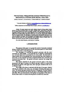
veloping the product is a prudent idea (favorable report) or unwise (unfavorable report). After the report, Google must make its own in-house decision to either invest the resources to develop the product or “kill it.” It may, in some instances, depending upon the potential upside of a highrisk investment, decide to go against the wisdom of the consultant’s findings and market the product. Conversely, on rare occasions, Google may also decide to drop a product even if it receives a favorable report. Organizing the Empirical Data Google wishes to design a decision tree to help organize and display the logical sequence of options and risky events that it faces with Robot. Additionally, the valuable experience gained over the years with similar, web-based products they have marketed will also be used in the current product assessment. The cost for the project, should Google decide develop it, is estimated at $100 million, however the likely revenues it could generate is estimated to be over $300 million within the first few years, based on the multitude of worldwide users they envision in their market. Consultant fees to conduct this extensive analysis is $7.5 million and will take approximately a 1-2 month time period to complete. Google reasons that this delay will also likely decrease the market share and corresponding revenue by approximately 10 percent but that it might be worth it to have a better idea of the risk involved provided by the consultant assessment. A summary of the cash flows is shown in Table 1. Next, Google digs into the details of the risk experiences with their past efforts to gain greater insight on how to

TABLE 1.

GOOGLE'S CASH FLOW ESTIMATES FOR ROBOT

proceed with this new product. A decision tree using Excel add-in TreePlan® that incorporates these cash flows is shown in Figure 1. Next, information needs to be gathered that will allow filling in the missing probabilities.


2


ICELW 2011

Google’s “Probability Tree” of Past Experiences During its relatively short, historically successful existence, Google has launched forty new products that fall into the same general arena as Robot. These products have been judged as successful if a minimum return on investment of at least 10 percent is realized—or unsuccessful if not realized. Google has never carefully analyzed these experiences including how accurately the consultant group has forecasted the product outcome, i.e., did their favorable reports usually result in a successful product or was it closer to hit and miss? Google discovers the following facts:

2.

return on investment. However, they correctly reason that one successful product pays for the unintended folly of several unsuccessful products. Of the 8 products that ultimately turned out to be successful, 7 of the 8 received favorable reviews, as did 3 of the ultimately unsuccessful products—29 out of the 32 unsuccessful products were correctly assessed with unfavorable reports.

Standard Introduction to Bayes’ Theorem: Using Event Probabilities

Figure 1. Google's Decision Tree for Robot Using TreePlan.

1.

There were 40 previous products, but only 8 were deemed successful, i.e., achieved at least a 10 percent

At this point, the empirical findings are translated into a probability tree, e.g., 8 of the 40 projects are successful so


3


ICELW 2011

P(S) is equal to 8/40 or 0.200; 7 of the 8 successful products were assessed favorably so P(F/S) is 7/8 or 0.875; and 29 of 32 unsuccessful products were given unfavorable reports by the consultant so P(S’/F’) equals 29/32 or 0.906, etc. The completed probability tree is shown in Figure 2. It is essential to point out the discrepancy between the probabilities needed to solve Robot’s decision tree of Figure 1 and the non-chronological probabilities in the probability tree of Figure 2. Although the path probabilities include the same combination of events, the sequence is not. This incongruity is corrected using Bayes’ Theorem. As an example of the procedure, suppose we want to determine the probability that a product will be successful if it receives a favorable report, P(S/F). Using Bayes’ Theorem, you would need to calculate the following intimidating relationship to revise the probability tree values using

It is also important to clarify the meaning of the numerator and denominator to further enlighten the student, e.g., the ratio represents the portion of favorable forecasts that are ultimately successful (numerator) while all the ways in which favorable forecasts can occur—both the successful as well as unsuccessful components—are represented in the denominator. This is, arguably, not an intuitive approach for most, and is often met with a restrained response from most student audiences. An alternative, far more simple method is offered next that retains the natural frequencies of the past experiences originally available to construct the

probability tree. Alternative Introduction to Bayes’ Theorem: Using Natural Frequencies From the information provided from Google’s previous 40 product launches, a probability tree identical in structure to Figure 2 is developed except this approach preserves and uses only the natural frequencies of the described historical events without converting the information into probabilities (Figure 3). Only three steps are used in this simplifying approach to the revision of probabilities using Bayes’ Theorem: Step 1.Choose any one of the two events at each chance node to revise, e.g., P(S), P(F), P(S/F), and P(S/F’). Step 2. For each event selected, identify and highlight the key natural frequencies that define the desired revised probability. Step 3. Form the appropriate fraction and convert it into the desired, revised probability. Voila! You’ve just used Bayes’ Theorem. Illustrated examples of the natural frequency method is applied to the four probabilities discussed in Step 2: EXAMPLE #1. What proportion of past product launches were successful, P(S)? BAYES REVISION: The only relevant event is the outcome of “success.” There were a total 8 successful products out of 40, so P(S) is 0.200 or 20 percent (Figure 4). EXAMPLE #2. What proportion of times did the consultant write a favorable report, P(F)? BAYES REVISION: Again, only a single event to focus on here except you must be careful to make sure you have looked at all the ways it can occur. The consultant wrote a total of 10 favorable reports—7 times for successful products, and another 3 for unsuccessful products. So, P(F) occurs 10 out of 40 or 0.250—25 percent (Figure 5). EXAMPLE #3. When a favorable report was written, what proportion of times was the consultant correct, i.e., the product was ultimately successful, P(S/F)? BAYES REVISION: Although 10 favorable reports were written, only the 7 of the 10 that were for successful outcomes are of interest, i.e., P(S/F) is 0.700 or 70 percent (Figure 6).

Figure 2. Standard Probability Tree for Google's Previous Product Launches.


4


ICELW 2011

!

Figure 3. Google Probability Tree for Past Launches Using Natural Frequencies.

Figure 5. Highlighting Key P(F) Components in Probability Tree.

Figure 4. Highlighting Key P(S) Components in Probability Tree.

EXAMPLE #4. What is the chance that the consultant would write an unfavorable report and, if the product is developed, it beats the odds to become successful, P(S/F’)? BAYES REVISION: There were a total of 30 unfavorable reports written but only 1 out of 30 were associated with a successful product, i.e., the chance of P(S/F’) occurring is only 0.033—3.3 percent (Figure 7).

Figure 6. Highlighting Key P(S/F) Components in Probability Tree.

Solution to Google’s Robot Project These four, revised probabilities are easily substituted into the decision tree in Figure 1, the complementary values added completing the missing information, and the problem is solved (Figure 8). The solution shown in the bolded paths reveals that the best strategy for Google to employ is: (1) Hire the consultant, C. Then, (2) if the consultant predicts a favorable outcome for the product, P(F)—which only has a 25 percent chance of happening—develop the product, D or (3) if the consultant report is unfavorable, P(F’)— 3 times as likely

Figure 7. Highlighting Key P(S/F’) Components in Probability Tree.


5


ICELW 2011

to occur as not—do not develop the product, D’. So the assessment is to follow the advice of the consultant findings in any event and will result in an average profit of $26.00 million (compared to only $9.99 million) if they decide to face the decision setting without the consultant. It also shows that the accuracy of the consultant is 70.0 percent when they write favorable reports (70% successful projects) and almost 97 percent when they write unfavorable reports (96.7% unsuccessful projects) with an overall accuracy of 90.0 percent.

ADDENDUM: DOVETAILING BAYES’ THEOREM WITH SENSITIVITY ANALYSIS In addition to the Bayes’ probability revision, it is also possible to link the use of the prior probabilities of success, P(S), with the likelihood of this point estimate being insufficient for thoughtful business analysis. The opportunity of refining our information to establish confidence intervals provides the manager with greater insight of how resilient the strategy is to variations in this key parameter and adds a richer context of understanding to the overall study. It also provides a logical extension to embrace sensitivity analysis

Figure 8. Solved Decision Tree for Baseline Google Robot Project* *Note: Bolded path defines most desirable strategy.


6


ICELW 2011

in refining the use of decision trees with the probabilities established using Bayes’ Theorem. As an illustration, suppose the chance of success, P(S), is presented to the student as an approximate value, i.e., there is concern that in assessing the outcomes of Google’s previous projects, there might have been possible judgment errors of “success.” If that is a reasonable assumption, then what is the bandwidth around the point estimate value of success that would establish the most optimistic and pessimistic limits and, most importantly, how does this affect our ultimate strategy that used the consultant group to guide Google. Can we determine, in using the extreme values established by the 95% confidence interval, if we would change this strategy? Google originally experienced 8 successful product launches out of a total of 40. This 20 percent success rate is merely a point estimate, as suggested previously. What is needed now is to establish the error tolerance associated with this information. Assume that Google is comfortable using a 95 percent confidence interval—the most common value used in business analysis. If so, the maximum and minimum values of the chance for success, P(S), can be found. For proportions, let P(S)= and the confidence interval for our problem is determined by solving (2)

p = pˆ ± Z95%

( pˆ )(1 ! pˆ ) n

(2)

where Z95%=1.960 for the 95% confidence interval, n= sample size of 40, and = Google’s point estimate of product success, P(S)=0.200. The confidence interval is easily calculated

This is a very wide interval. Based on the experience of 40 previous projects, the estimate of P(S) shows an extremely volatile number, i.e., the ± 0.124 exceeds a 60% variation in the original point estimate value of 0.200. The Robot decision tree must now be resolved between the maximum (optimistic) and minimum (pessimistic) values for P(S) of 0.076 and 0.324, respectively to see if the optimal strategy shifts between C and C’. If not—if the strategy of selecting the consultant, C’, remains the preferred selection and the problem is not sensitive across the confidence interval range. Resolving Robot Using the Lower 95% Confidence Interval Value of P(S)=0.076

For the 40 projects, this would mean that the interpretation for success would be approximately 3 out of the 40 product launches (0.075 ! 0.076). If the forecast accuracies remain about the same then we need to adjust the historical data. There are 7 favorable reports written (3 are associated with successful products and 4, with unsuccessful products); 33 unfavorable reports (none with successful projects, all 33 with unsuccessful projects). Now we can revise our original decision tree to accommodate out minimum chance for success. We know that: P(F)=7/40=0.175 P(F’)=1-P(F)=0.825 P(S/F)=3/7=0.429 P(S’/F)=1-P(S/F)=0.571 P(S/F’)=0/33=0.000 P(S’/F’)=33/33 =1.000 The results using the minimal value for P(S) shows that we would still hire the consultant, C, even though the EV(C) has decreased to only $3.13 Million from the original $31.38 Million (Figure 10). The key finding is that the strategy is unchanged from our original decision. Resolving Robot Using the Upper 95% Confidence Interval Value of P(S)=0.324 If P(S)=0.324 we would logically assume that a little less than one-third of the original projects were successful or about 13 out of the 40. This would yield a P(S)=0.325— not precisely the upper limit value but close enough to represent a reasonably level of interpretational variation. The decision tree can now be updated since we know that:

Figure 9. Monster Past Project Outcomes and Predictions Adjusted for Lower Confidence Limit of P(S)= 0.076.

If P(S)=0.076 the decision tree probabilities need to be adjusted starting with our previous experience (Figure 9).


7


ICELW 2011

P(S)=0.325 P(S’)=1-P(S)= 0.675 P(F)=16/40=0.400 P(F’)=1-P(F)=0.600; P(S/F)=13/16=0.813 P(S’/F)=1-P(S/F)=3/16=0.187 P(S/F’)=3/27= 0.111 P(S’/F’)=1-P(S/F’)=24/27=0.889 The solution, using the maximum confidence interval value for P(S), shows that the strategy of selecting the consultant, C, is still preferred (Figure 11). A plot of EV(C) and EV(C’) in Figure 12 shows that the hire consultant strategy, C, dominates C’ across the 95 percent confidence interval range of P(S) . CONCLUSIONS

The comparative ease of replacing probabilities with the natural frequency of the event simplifies the use and understandability of probability trees and the application of Bayes’ Theorem for both student and teacher. A sense of scale, not present with the traditional use of probabilities, lends an illuminating and clarifying perspective to the usefulness of Bayes’ Theorem. Simplicity can be elegant—and size does matter in the application of this methodology. In addition, the opportunity to connect the application of Bayes’ Theorem with an often-overlooked need to establish the fact that many “calculations” of probabilities are often subject to human interpretation is established. The subsequent ease of linking Bayes’ teaching with the use of sensitivity analysis lends a additional layer of realism that sets aside the assumption that the information is adequately represented by point estimates alone.

Figure 10. Robot Decision Tree Using Lower Confidence Limit Value of P(S)=0.076.


8


ICELW 2011

Figure 11. Robot Decision Tree Upper Confidence Limit Value of P(S)=0.324.

Figure 12. Effect of P(S) on the Expected Values of Strategies C and C’.


9


ICELW 2011

REFERENCES [1]

[2]

[3] [4] [5]

[6]

Brown, R. (2005), The operation was a success but the patient died: Aider priorities influence decision analysis usefulness, Interfaces, Volume 35, Issue 6 (November-December), pp. 511-521. Casscells, W., Schoenberger, A., and Grayboys, T. (1978): "Interpretation by physicians of clinical laboratory results." New England Journal of Medicine, 299:999-1001. Dehaene, Stanislas (1997): The number sense: How the mind creates mathematics. Oxford University Press. Dawid, A. P. (2002): Bayes’s Theorem and Weighing Evidence by Juries, Proceedings of the British Academy, Volume 113: 71-90. Edwards, Ward (1982): "Conservatism in human information processing." In D. Kahneman, P. Slovic, and A. Tversky, eds, Judgment under uncertainty: Heuristics and biases. Cambridge University Press, Cambridge, UK. Gigerenzer, Gerd and Hoffrage, Ulrich (1995): "How

to improve Bayesian reasoning without instruction: Frequency formats." Psychological Review. 102: 684-704. [7] Hoffrage, Ulrich and Gigerenzer, Gerd (1998): “Using natural frequencies to improve diagnostic inferences.” Academy of Medicine: 73(5): 538-40. [8] Kaye, D. H. and Koehler, J. J (1991): Can Jurors Understand Probabilistic Evidence? Journal of the Royal Statistical Society (Series A), 154, Part 1, pp. 75-81. [9] TreePlan® Excel add-in software, http://www.treeplan.com/treeplan.htm [10] Yudkowsky, Eliezer S., An Intuitive Explanation of Bayesian Reasoning, ©2003. http://yudkowsky.net/rational/bayes AUTHOR Joel Oberstone, University of San Francisco, School of Business and Professional Studies, Professor of Business Analytics, 2130 Fulton Street, San Francisco, CA 94117, Email: [email protected]


10