Name=queuen. Tokens = 1. Name=Machine ... Name=queuen. Name=Machine
.... Electronic Notes in Theoretical Computer Science 72(2). 2. Bottoni, P., Koch ...
Automated Model Transformation and its Validation using AToM3 and AGG Juan de Lara1 and Gabriele Taentzer 2 1
Escuela Polit´ecnica Superior Ingenier´ıa Inform´atica Universidad Aut´onoma de Madrid
[email protected] 2 Computer Science Department Technische Universitat Berlin Berlin, Germany
[email protected]
Abstract. Complex Systems are characterized by components that may have to be described using different notations. For the analysis of such a system, our approach is to transform each component (preserving behaviour) into a single common formalism with appropriate analysis methods. Both source and target notations are described by means of meta-modelling whereas the translation is modelled by means of graph transformation. During the transformation process, the intermediate models can be a blend of elements of the source and target notations, but at the end the resulting model should be expressed in the target notation alone. In this work we propose defining also a meta-model for the intermediate process, in such a way that we can apply some validation methods to the transformation. In particular, we show how to proof functional behaviour (confluence and termination) via critical pair analysis and layering conditions, and discuss other desirable properties of the transformation, namely: syntactic consistency and behaviour preservation. The automation of these concepts has been carried out by combining the AToM3 and AGG tools.
Keywords: Meta-Modelling, Graph Transformation, Multi-Formalism Modelling.
1 Introduction The motivation of this work is the modelling, analysis and simulation of multi-formalism systems. These have components that may have to be described using different notations, due to their different characteristics. For the analysis of certain properties of the whole system, or for its simulation, we transform each component into a common single formalism, where appropriate analysis or simulation techniques are available. The formalism transformation graph (FTG) [4] may help in finding such formalism. It depicts a small part of the “formalism space”, in which formalisms are shown as nodes in the graph and the arrows between them denote a homomorphic relationship “can be mapped onto”, using symbolic transformations between formalisms. These transformations may lead to a loss of information. Nonetheless, by performing the transformation
we are able to solve questions that were harder or impossible to answer in the source formalism. Other arrows depict simulation and optimization (arrows starting and arriving to the same formalism). Our approach is to define the syntax of the formalisms via meta-modelling, and to formally express transformations between formalisms by means of graph transformation. That is, starting with a graph G 1 in formalism F1 , applying a formalism transformation we obtain a graph G 2 expressed in formalism F 2 . Some work regarding model transformation in the context of multi-formalism modelling and simulation has already been done (see for example [5] and [4]) where not only formalism transformation, but simulation and optimization arrows have been modelled as graph transformation rules. Thus a number of model transformations have already been modelled using the AToM 3 tool [4]. The main contribution of the present work is proposing the creation of meta-models also for the intermediate models during the transformation (that is, for the transformation arrows in the FTG), and showing fundamental properties of the transformation process. In particular we proof confluence (proving that the result of the transformation is deterministic), termination (by modifying the layering conditions proposed in [3]), consistency (the resulting models should be valid instances of the target formalism meta-model) and behavioural equivalence of source and target models. In addition, a prototype for the automation of the whole process has been realized by combining the AToM3 [4] and AGG [19] tools. Although using graph transformation has been widely used for expressing model transformations, there are not many attempts to formally validate the transformation process. For example, in [1] an environment is presented to define Function Block Diagrams models. They can be executed by transforming them into High Level Timed Petri Nets using graph grammar rules but no proofs are given for the properties of the transformation. In [11] critical pair analysis was used to proof confluence of a transformation from Statecharts into CSP (a textual formalism). The present work is a step further, as here the target formalism is also graphical, we provide a meta-model for the intermediate models arising during the transformation and proof further transformation properties.
2 A Meta-Model for the Transformation Process During the process of transforming a model from formalism F 1 into formalism F2 , the intermediate models can have elements of both formalisms, as well as extra elements. These are typically new links between elements of both formalisms, and auxiliary entities. In a correct formalism transformation, at the end of the transformation process the resulting model should be expressed in formalism F 2 alone. If we formalize the syntax of both source and target formalisms using type graphs (a concept similar to a metatypeF
tra
∗
typeF
F 12 model, see below), this can be expressed as: T G F1 ←−1 G1 =⇒ G2 −→2 F2 . That is, there is a typing morphism type F1 from G1 to the type graph of formalism F1 (T GF1 ). At the end of the transformation (expressed as the set of production rules traF 12 = {p1 , ..., pn }), there is a typing morphism type F2 from G2 to the type graph of formalism F2 (T GF2 ).
2
In order to formalize the kind of manipulations that can be performed during the process, a type graph T G F12 should be defined for the graphs derived during the transformation process. Both T G F1 and T GF2 should have injective morphisms to T G F12 . By enforcing these morphisms, we make sure that if graph G 1 is typed over T GF1 it is also typed over T G F12 , and the same for graph G 2 . This can be sketched in the diagram in Figure 1.
F2 / T GF12 o T GF2 ; O cHH O v v H HH vv v H HH type v typeF12 vv HH F12 typeF1 typeF12 typeF2 vv HH v HH v v H v HH v HH vv vv pi pj pk pl / ... / G12 / ... / G2 G1
T GF1
O
F1
Fig. 1. Typing in the Formalism Transformation Process.
For a graph G 1 typed on T GF1 , the typing should be the same on type F12 , that is F1 ◦ typeF1 = typeF12 . A similar situation happens with a graph G 2 typed on T GF2 (F2 ◦ typeF2 = typeF12 .) Usually, the type graph T G F12 is the disjoint union of T G F1 and T GF2 , and possibly some auxiliary nodes and connections that may be used during the transformation process. In practice, in order to define a formalism, one sets additional constraints on type graphs. Typically, these include constraints on the multiplicities of relationships as well as additional constraints expressed either textually (in the form of OCL formulae for example) or graphically (as visual OCL constraints [2] for example). Throughout the paper we refer to the type graph with additional constraints as “meta-model”. Thus, the meta-model for formalism F 12 is formed by a type graph T G F12 as described before, together with the constraints of both source and target meta-models, plus additional constraints on the new elements in T G F12 − (T GF1 ∪ T GF2 ). For this approach to be easier to apply, we can make the constraints coming from the meta-model of formalism F1 less restrictive. If a model M 1 meets the constraints of the meta-model for F 1 , it will meet the constraints of meta-model for formalism F 12 , as they are less restrictive. On the contrary, we cannot relax the constraints coming from the meta-model of formalism F2 as then we cannot be sure that at the end of the transformation the resulting model will meet the constraints of formalism F 2 . We give an example of these concepts in the following section.
3 An Example: From Process Interaction to TTPN Suppose we want to transform a certain discrete event formalism [8] (in the ProcessInteraction style [10]) into Timed Transition Petri Nets (TTPN) [15], as the latter formalism has analysis methods not usually available for Process-Interaction, such as the 3
ones based on the reachability graph or structural analysis. The Process Interaction notation we consider here is specially tailored to the manufacturing domain. Models are composed of a number of machines interconnected via queues in which pieces can be stored. Machines can be in state Idle or Busy and take a number of time steps (attribute Tproc) to process each piece. They are also provided with attribute Tend which signals the time at which they will finish the processing of the current piece. Pieces are produced by generators at certain rates (given by the Inter Arrival Time IAT). Generators are also provided with an additional attribute (Tnext) which signals the time of the next piece generation. A global timer controls the current simulation time (Time attribute) and the final time (FinalTime attribute). This meta-model is shown to the left of Figure 2, enclosed in the dotted rectangle labelled as “Process Interaction Meta-Model”. The direction of connections is shown as small arrows near the connection name. Timed Transition Petri nets (TTPN) are like regular black and white Petri nets, but transitions are associated a delay (“Time” attribute), in such a way that, before firing, they have to be enabled for a number of units of time equal to the delay. In this work we assume atomic firing (tokens remain in places until transitions fire), age memory (each transition keeps the actual value of its timer when a transition fires), and single server semantics (each transition has only one timer). We have also added attribute Tleft to transitions, which controls the time it remains for the transition to be fired (in case the transition is enabled). Its value should be in the interval [0..Time]. The TTPN meta-model has been depicted to the right of Figure 2 enclosed in the dotted rectangle labelled as “TTPN Meta-Model”. generator2transition > 0..1
Transition Timer nextPiece >
0..*
0..1
Name: string
0..1 Tcreation: float
0..*
0..1
first >
generator2queue
0..1
0..1
pieceInMachine
>
>
postDomain >
Piece
IAT: float Tnext: float
0..1
last > 0..1
0..1
Queue Name: string 0..1
0..1
Machine
0..* < preDomain
0..1
Generator
Name: string Time: float Tleft: float
Time: float FinalTime: float
0..*
0..*
< output 0..* 0..* Name: string State: enum={idle, busy} input >
0..1
< busy
0..1
0..*
0..1
< idle
0..1 Tokens: integer
Tproc: float
0..* Tend: float
Place Name: string
0..1 < place2queue
Process Interaction Meta−Model
TTPN Meta−Model
Meta−Model for Transformation from Process Interaction into TTPN
Fig. 2. Meta-model for the Transformation from Process Interaction into TTPN.
The meta-model for the transformation process is also depicted in Figure 2, and is the disjoint union of the elements of both meta-models together with some extra links (shown in bold) that show how elements of both notations are related during the trans4
formation process. We have relaxed some multiplicity constraints, in such a way that relationships “output” and “input” between machines and queues have been assigned multiplicity “0..*” in the side of the queues. In the original Process Interaction metamodel, this multiplicity was “1..*” (each machine should have at least one input queue and at least one output queue). We have performed this relaxation in order to make the overall transformation process easier (as during the transformation process, machines will become unconnected). In the TTPN formalism we represent pieces as tokens. The latter are represented as attributes of places. Pieces are generated by transitions (generators in the process interaction notation). A queue is represented by a place, and machines by two places representing the Busy and the Idle states. Once this meta-model is defined, we can model the formalism transformation. This can be applied to any process interaction model, as they are also typed over the metamodel for the transformation as stated in the previous section. Figures 3, 4, 5 and 6 show the rules for the transformation. Nodes and edges in the left hand side (LHS), right hand side (RHS) and negative application condition (NAC) are assigned the same number if they represent the same object in the matching. The idea of the transformation is to provide each Process Interaction element with its corresponding Petri net element, transfer the connectivity of the Process Interaction elements to the Petri net, and then erase the Process Interaction elements. Rule 1 is applied to a generator not processed before (this is expressed with the NAC), and attaches a Petri net transition to it. The delay of this transition is set to the Inter Arrival Time (IAT) specified in the generator. The time it remains for firing is set to the time of the next generation event (signalled by Tnext attribute of the generator) minus the current simulation time (attribute Time of the timer.) In this way, the transition will fire at the same intervals (each IAT units of time) in which the generator produces a piece, including the first time (in Tleft units of time). Rule 2 attaches a Petri net place to each queue. Rules 4 and 5 will assign to this place as many tokens as pieces are connected to the queue. The third rule attaches two Petri net places to each machine. They represent the machine states Idle and Busy. The rule puts a token in the place representing the Idle state, although this can be changed later by rule 6. As the machine can be in only one state at the same time, later we will make sure that the number of tokens in both places is exactly one, using a well known structural property of Petri nets for capacity constraint. As stated before, rules 4 and 5 (in Figure 4) convert the pieces stored in the queues into tokens for the place associated with the queue. Rule 4 is used when the queue has more than one stored piece, while rule number 5 is used to delete the last piece in the queue. By converting pieces into tokens we are losing information, as pieces have information about their creation time (attribute Tcreation). This information loss is acceptable if we are not interested in using that information in the target formalism. Rule 6 is applied when a machine is Busy, that is, it is processing a piece. In this case, the piece is removed and the token is passed from the place representing the Idle state to the place representing that the machine is Busy. We simply erase the piece inside the machine, rule 12 will configure the remaining time for firing the Petri net transitions associated with the end of processing of the machine. 5
Rule 1: Convert Generators
NAC
LHS
Name= Time=
1 g2t
IAT= Tnext= Generator
1
g2t
Time=sTime FinalTime=sFinal
IAT=vIAT Tnext=vTnext Transition
Name="Gen"+vIAT Time=vIAT Tleft=vTnext−sTime 2
RHS 2
1
Generator
Time=sTime FinalTime=sFinal
IAT=vIAT Tnext=vTnext
Timer
Generator
Transition
Timer
Rule 2: Convert Queues
NAC
LHS
Name= Tokens=
Name=
RHS
Name=vName
Name=vName Tokens=0
Name=vName
p2q Queue
1
p2q Queue
1
Place
Queue
1
Place
Rule 3: Convert Machines
NAC
LHS
Name= Tokens=
1 Name= State= Tproc= Tend=
Place busy
Name= Tokens=
Machine
Name=vName+" busy" Tokens=0
RHS
1
1
Name=vName State=vState Tproc=vTproc Tend=vTend
Name=vName State=vState Tproc=vTproc Tend=vTend
Machine
busy
Place
idle
Place
Name=vName+" idle" Tokens=1
Machine
idle
Place
Fig. 3. First three rules in the Transformation from Process Interaction into TTPN. Rule 4: Delete Pieces
Rule 5: Delete Last Piece
LHS Queue
RHS Name=pName Tokens=pTokens
Name=qName
LHS Name=pName Tokens=pTokens+1
Name=qName
Queue
p2q Place
1
Name= Tcreation= nextPiece
Place
1
Piece
Name=piName Tcreation=piCr
1
3
Place
First
Name= Tcreation=
4
2 Place
3
Last
Name=pName Tokens=pTokens+1
Name=qName
p2q
2 3
Last
Piece
Queue
p2q
2 3
Last
RHS Name=pName Tokens=pTokens
Name=qName
p2q
2 1
Queue
Piece
Piece
Name=piName Tcreation=piCr
4
Rule 6: Delete Piece in Machine
LHS
Machine
1
Name=vName State=Busy Tproc=vTproc Tend=vTend 2 idle Place
busy
4
RHS Tcreation=
Piece
2 idle
3 Place
Place
5 Name=iName Tokens=iTokens
Machine
1
Name=vName State=Busy Tproc=vTproc Tend=vTend
piecInMac Name=
busy
4
3 Place
5
Name=bName Tokens=bTokens
Name=iName Tokens=0
Name=bName Tokens=1
Fig. 4. Second set of Rules in the Transformation from Process Interaction into TTPN.
The third set of rules (depicted in Figure 5) is used to connect the Petri net elements according to the connectivity of the attached Process Interaction elements. Rule 7 connects the transition attached to each generator with the place attached to the connected queues. This rule is applied once for each queue attached to each generator. The connection between the generator and the queue is deleted to avoid multiple processing of the same generator and queue. Rule 8 connects (through a transition) the associated place of an incoming queue to a machine with the places associated with it. For the transition to be enabled, at least one token is needed in both the place associated with the queue (which represents an incoming piece), and the place representing the Idle state of the machine. When the transition fires, it changes the machine state to Busy and removes a token from the place representing the queue. If the rule is executed, then the queue is also disconnected from 6
the machine to avoid multiple processing of the same queue and machine, but this rule is applied for each queue attached to each machine. A similar situation (but for output queues) is modelled by rule 9. It connects (through a transition) the places associated with the machine to the place associated with an output queue. For this transition to be enabled, the place representing the Busy state should have at least one token. When the transition fires, it changes the machine state back to Idle and puts a token in the place representing the queue (modelling the fact that a piece has been processed by the machine). If this rule is executed, the queue is also disconnected from the machine, in the same way as the previous rule. Finally, rule 10 models a similar situation to the previous one, but in this case the machine is busy. The only change with respect to the previous rule is that we have to configure the Petri net transition with the units of time remaining for firing. This is calculated as the time at which the machine finishes the processing of the piece minus the current simulation time. Rule 9: Connect Output Queues Idle
Rule 7: Connect Generators Name=tName Time=tTime Tleft=tTleft 3
LHS 1 2
1
g2t
IAT=gIAT Tnext=gTnext Generator
Name=tName Time=tTime Tleft=tTleft 3 2
RHS
Generator
RHS Machine
2
g2t
IAT=gIAT Tnext=gTnext Transition
LHS
post Transition
5 idle
g2q
Name=pName Tokens=pTokens
Queue
Name=pName Tokens=pTokens
Queue
Place
busy
3 p2q
5 idle
7 Place
Place
4
busy
3 p2q 7
4
p2q
5
5 Place
6
Name=qName
4
6
Name=qName
Name=iName Tokens=iTokens
Place
Name=pqName Tokens=pqTokens
Name=bName Tokens=bTokens
Name=iName Tokens=iTokens
post
Machine
2
5 idle
Place
Place
4
busy
6
Name=vName State=vState Tproc=vTproc Tend=vTend
3 p2q
7 Place
Machine
2
Name=qName
1
Name=vName State=vState Tproc=vTproc Tend=vTend
3 p2q
5 idle
Place
Place
4
busy
6
8
Rule 10: Connect Output Queues Busy
LHS
Name=iName Tokens=iTokens
Name=bName Tokens=bTokens
pre Name=iName
Name="inp "+vName Time = 0 Tleft = 0 Transition
Tokens=iTokens
Name=bName Tokens=bTokens
5 idle Place
busy
6
Name=qName
1
Name=vName State=Busy Tproc=vTproc Tend=vTend
Place
8 Name=pqName Tokens=pqTokens
RHS Machine
2
7
pre
Name=pqName Tokens=pqTokens
pre
Name="out "+qName Time = Tproc Tleft=Tproc
RHS inp
Name=pqName Tokens=pqTokens
Name=bName Tokens=bTokens
post
LHS Name=qName
4
8
Rule 8: Connect Input Queues
1
Place
Place
6
8 p2q
Name=qName
1
Name=vName State=Idle Tproc=vTproc Tend=vTend
out
Place
6
Machine
2
Name=qName
1
Name=vName State=Idle Tproc=vTproc Tend=vTend
Machine
2
Name=qName
1
Name=vName State=Busy Tproc=vTproc Tend=vTend
out
9 3 p2q
Time=sTime FinalTime=sFinal
7 Place
Place
4
post
5 idle Place
busy
6
3 p2q 7 Place
Place
Timer
4
8
8 Name=iName Tokens=iTokens
Name=bName Tokens=bTokens
Name=pqName Tokens=pqTokens
Name=iName Tokens=iTokens post
Name=bName Tokens=bTokens pre
Name=pqName Tokens=pqTokens 9
post
Name="out "+qName Time = Tproc Tleft=vTend−sTime
Time=sTime FinalTime=sFinal
Fig. 5. Third set of Rules in the Transformation from Process Interaction into TTPN.
The last set of rules (shown in Figure 6) simply removes the Process Interaction elements, once the connectivity between these elements has been transfer to the Petri net elements. We want rules 11 - 13 to be applied once the Process Interaction elements are unconnected. We take advantage of the dangling edge condition of the Double Pushout Approach [17] for this. In this way, if any Process Interaction element has some connection, the rules cannot be applied, and we make sure that rules 7-10 have been applied as many times as possible. The timer can only be deleted once we have processed all generators and pieces, otherwise we may need it in rules 1 and 10. With the NACs, we make sure that the timer is deleted once machines and generators have been processed and thus deleted. The transformation has four well-defined phases: creation of the target formalism elements (Figure 3), deletion of pieces (Figure 4), connection of the target formalism 7
Timer
Rule 13: Delete Machines
Rule 11: Delete Generators
LHS
Name=tName Time=tTime
RHS
LHS
Name=tName Time=tTime
1
Generator
Transition
Transition
idle
Rule 12: Delete Queues
Place
Name=
2 Name=bName Tokens=bTokens
busy Place
1
2 1
1
Name=iName Tokens=iTokens
p2q
Name=pqName Tokens=pqTokens
Place
1
Name=iName Tokens=iTokens
RHS
LHS
Place
Name=vName State=vState Tproc=vTproc Tend=vTend
g2t
IAT= Tnext=
RHS Machine
1
Name=pqName Tokens=pqTokens
Name=bName Tokens=bTokens
Rule 14: Delete Timer
NAC
NAC
Name= State= Tproc= Tend=
LHS
RHS
Time= FinalTime=
IAT= Tnext=
Timer
Generator
Machine
Fig. 6. Fourth set of Rules in the Transformation from Process Interaction into TTPN.
elements (Figure 5) and finally deletion of the source formalism elements (Figure 6). Although not strictly necessary, we can use a simple control structure for rule execution based on layers. Thus, we assign rules in each phase to different layers (numbered from 0 to 3, this numbering will be used later in the validation process). Rules in each layer are applied as long as possible. When none of the rules of layer n is applicable, then rules of layer n + 1 are considered. The graph grammar execution ends when none of the rules of the highest layer is applicable. As an example, Figure 7 shows the transformation into TTPN of a model representing a machine which can produce defective pieces, which then should be fixed by another machine and sent back for their processing by the first machine.
Process Interaction Model
Time=24 FinalTime=30
IAT=12 Tnext=36
Name=Piece1 Tcreation=0.0 Name=Input
first Name=Process State=Busy Tproc=10.0 Tend=34
Name=Rework
last
Name=Piece2 Tcreation=12.0
Name=Good Pieces
Name=Piece3 Tcreation=24.0
Name=Defect
Name=Fix State=Busy Tproc=5.0 Tend=27
Graph Transformation
Name=Gen12 Name=Input Time=12 Tokens=0
Name=inp Process Time=0 Tleft=0
TTPN Model Name=Process IdleName=out Process Tokens=0 Time=10 Tleft=10
Name=Rework Tokens=0
Name=inp Process Name=Process busy Tokens=1 Time=0 Tleft=0
Name=out Process Time=10 Tleft=10
Name=Good Pieces Tokens=1 Name=inp Fix Time=0 Tleft=0
Name=Fix Idle Tokens=0 Name=out Fix Time=5 Tleft=3
Name=Defect Tokens=0 Name=Fix Busy Tokens=1
Fig. 7. Transforming a Process Interaction Model into an equivalent TTPN model.
8
4 Validating the Transformation Process For a formalism transformation to be useful one needs to ensure that it has certain properties. The first one is functional behaviour, which can be further decomposed in confluency and termination, and assures that the same output is obtained from equal inputs. The second one is consistency, that is, ensuring that models resulting from the transformation are valid instances of the target meta-model. Finally, usually one would like the source and target formalisms to be equivalent in behaviour. These properties are examined in the following sections. 4.1 Functional Behaviour Critical pair analysis is known from term rewriting and is usually used to check if a term rewriting system has a functional behaviour, i.e. is confluent. Critical pair analysis has been generalized to graph rewriting [14], and formalizes the idea of a minimal example of a conflicting situation. From the set of all critical pairs we can extract the objects and links that cause conflicts or dependencies. A system is locally confluent if all conflicting pairs are confluent, that is, they are extendible by transformation sequences leading to a common successor graph. In [11], critical pair analysis was extended to attributed graph transformation. In the area of formalism transformation, we are interested in transformations that are confluent, in the sense that a given model in the source formalism should be deterministically transformed into a unique model in the target formalism. For that purpose, we can use critical pair analysis, which was automated in the AGG tool. For the example we are dealing with, AGG finds two pairs of rules in conflict: rule 1 with itself, and rule 10 and itself. In both cases, the conflict could arise in multiple matchings in two common graphs but with two different timers. As in valid Process Interaction models one cannot have two timers, these critical pairs cannot happen in practice, and the transformation is confluent. However as this restriction on the multiplicity of timers could not be explicitly conveyed in the type graph, AGG found this situation as a potential conflict. Note also that only rules in the same layer have to be checked for conflicts. Termination is undecidable in general, but for the concrete example we are dealing with, we can show that the transformation terminates. Starting from finite, correct models in the Process Interaction formalism, the rules can only be applied finitely many times. Rules 1-3, which associate Petri net elements with the Process Interaction blocks, can only be applied once for each block. This is controlled by the NACs. Rules in Figure 4 erase pieces, so their application terminates if there are a finite number of them in the initial model (which is true since the model is finite). Rules 7-9 can be applied only a finite number of times, since they are applied once for each relationship generator2queue, input and output in the original Process Interaction model. Finally, rules 10-12 also terminate, as they remove Process Interaction elements, and there are a finite number of them. Note also, that we do not have cycles: no new Process Interaction nodes or relationships are created, which could trigger the iterative execution of the rules. 9
In [16] termination is proved by defining a layering conditions, which all rules must fulfil. This concept was further refined in [3], where the following layering functions are defined: 1. cl, dl : L → N are total functions which assign each label (that is, each element) a unique creation and a unique deletion layer such that ∀l ∈ L : 0 ≤ cl(l) ≤ dl(l) ≤ n. 2. rl : R → N is a total function which assigns each rule a unique layer. The execution of a graph grammar terminates if all rules r ∈ R with rl(r) = k fulfil the following layering conditions: 1. 2. 3. 4. 5.
The host graph is finite, r deletes only nodes and edges with labels l such that dl(l) ≤ k, r creates only nodes and edges with labels l such that cl(l) > k, r deletes at least one node or edge, r uses only N ACs over nodes and edges with labels l such that cl(l) ≤ k.
We cannot apply directly this concept, because we both create elements of the target formalism (in rules 1-3, layer 0), and delete elements of the source formalism and it is not possible to find an appropriate layer order. But still, we can modify the previous concept (which was used for parsing pourposes) to make it suitable for formalism transfomation grammars. We can classify the layers of our grammar either as deletion or creation layers. The former delete elements of the source formalism, while the latter create elements of the target formalism. For the deletion layers we can use the previous layering conditions. In our example, layers 1-3 are deletion layers and we can meet the layering conditions specifying the layering functions as follows: dl(target) = cl(source) = dl(source) = dl(aux) = 1, cl(target) = cl(aux) = 2. Where source and target are the labels of nodes and edges of source (Process Interaction) and target (TTPN) formalisms, while aux refers to the auxiliary nodes and edges included in the meta-model for the transformation (busy, idle, place2queue and generator2transition edges in our example). For the creation layers in which we create new elements of the target formalism (such as layer 0 in the example), we can define new layering conditions: 1. 2. 3. 4.
The host graph is finite, r deletes only nodes and edges with labels l such that dl(l) ≤ k, r creates nodes or edges with labels l such that cl(l) > k, ∃m : N → R with m(x) = y ∀x ∈ N − n(L) and y ∈ R − r(K),
where N is the NAC, L is the LHS, R is the RHS and we have the usual morphisms n l r in the Double Pushout Approach N ←− L ←− K −→ R. The new conditions 1, 2 and 3 do not change with respect to the previous ones. Deletion of at least one edge or node is not required, but we must ensure that the application of rules is still bounded. This is expressed with condition 4, which states that if a rule creates any element y, this element should explictly appear in the part of the N AC which is not in the LHS (N −n(L)). Moreover, there should be a morphism between the newly created elements 10
and that part of the NAC. This ensures that the rule can be applied only once. That is, these new layering condition state sufficient conditions for termination. In our example, rules 1-3 belong to layer 0, which is a creation layer, for which we should check the new layering conditions. These are satisfied, as rules create elements of the target and aux layers (cl(target) = cl(aux) = 2) and there is a morphism from each N AC to the newly created elements, in such a way that the rules can be applied only once for each element of the source formalism. This concept of creation and deletion layers is not only applicable to the specific example proposed in this paper, but is also applicable to any other graph grammar. 4.2 Consistency With respect to consistency (that is, the final models are correct instances of the TTPN meta-model alone), all rules produce model elements correctly typed according to the target meta-model. Note that if the transformation terminates, it means that rules 11-13, which delete Process Interaction elements connected to TTPN elements are no longer applicable. This means that either we do not have Process Interaction elements or they are not connected to the TTPN elements (so that rules 11-13 cannot be applied). The latter is not possible, as we connect each Process Interaction element with a TTPN element by the application of rules 1-3. Finally, the TTPN elements are correctly connected, as the only rules that connect them are rules 7-10, and these connections are not modified later. 4.3 Behavioural Equivalence With respect to behavioural equivalence, Figure 8 shows how the Process Interaction constructs are translated into TTPN. We (informally) show that this is their intended meaning. The situation shown in Figure 8 (a) shows the conversion of a queue with a number of attached generators. In the meta-model it is specified that a queue can receive connections from zero or more generators. In a TTPN model, this is equivalent to having a place connected to one transition for each generator connected to the original queue. This is exactly what we obtain when transforming the left hand side of Figure 8 (a), by means of the rules indicated on top of the arrow. Figure 8 (b) shows the conversion of a number of queues incoming to a machine. A machine can have one or many incoming queues connected to it. What we want to express in an equivalent TTPN model is that we have a connection from each place representing each queue to the places representing the machine through independent transitions. Each transition connecting the places representing the queues are in conflict when the machine is idle. This means that only one of the queues can put a piece in the machine. That is, we have modelled mutual exclusion of the machine. In a similar way, figures 8 (c) and (d) model the translation of the output queues connected to a machine. Machines can have one or more output queues. What we want to model here is that only one queue receives the processed piece. This is achieved by creating an independent transition for each queue, and making them synchronized (same associated time) and in conflict, so all of them will be enabled at the same time, but only one of them will fire. 11
n
(a)
IAT=gIAT1 Tnext=gTnext1
n
...
Rule 1 (n times) Rule 2 Rule 7 (n times) Rule 11 (n times) Rule 12 Rule 14
IAT=gIATn Tnext=gTnextn
Time=sTime FinalTime=sFinal
Name="Gen "+gIAT1 Time=gIAT1 Tleft=gTnext1−sTime
...
Name=queue1
Name=queue1
(b)
Name=queue1 Tokens = 0
Name=queue1
...
n
Rule 3 Rule 2 (n times) Rule 8 (n times) Rule 12 (n times) Rule 13
Name=Machine State=Idle Tproc=t1 Tend=tend
Name=queuen
... Name=Machine Busy Tokens = 0
(c)
Name=Machine State=Idle Tproc=t1 Tend=busy
Name=queue1
n
... Name=queuen
Rule 3 Name=Machine Idle Rule 2 (n times) Tokens = 0 Rule 10 (n times) Rule 12 (n times) Rule 6 Rule 13 Rule 14
Name=inp Machine Time = 0 Tleft = 0 Name=out Machine Time = t1 Tleft = tend−sTime Name=queue1 Tokens = 0
...
n Name=queuen Tokens = 0
Name=Machine Busy Name=out Machine Tokens = 1 Time = t1 Tleft = tend−sTime
Name= Tcreation=
(d) Name=Machine Idle Tokens = 1
Name=queue1
Name=Machine State=Idle Tproc=t1 Tend=tend
Name=inp Machine Time = 0 Tleft = 0 Name=Machine Idle Tokens = 1
n
Name=queuen Tokens = 0
Time=sTime FinalTime=sFinal
Name="Gen "+gIATn Time=gIATn Tleft=gTnextn−sTime
...
n Name=queuen
Rule 3 Rule 2 (n times) Rule 9 (n times) Rule 12 (n times) Rule 13
Name=out Machine Time = t1 Tleft = t1 Name=queue1 Tokens = 0
... n Name=queuen Tokens = 0 Name=Machine Busy Name=out Machine Tokens = 0 Time = t1 Tleft = t1
Fig. 8. Equivalent TTPN constructs and Their Translation.
5 Realization in AToM3 and AGG The previous transformation has been modelled with AToM 3 . As critical pair analysis is available in the AGG tool [19], we extended AToM 3 with the capability to export graph grammars in the XML format of AGG (for the moment this exchange is unidirectional). This was not a straightforward task, as AToM 3 is implemented in Python, whereas AGG is implemented in Java, and (textual) applicability conditions as well as attribute computations are expressed in Python and Java respectively. Additionally, the attribution concept has a different philosophy in both tools. In AGG variables are assigned to attributes (possibly the same variable to more than one attribute, which means that they should have the same value). These variables can be used in RHS nodes’ attributes to calculate new values and in additional applicability conditions, expressed in Java. In AToM3 however, there is an API to access nodes (via labels) and its attributes, and there are applicability conditions at the level of rules. In these conditions we can use the AToM3 API to formulate expressions on combinations of several attributes. In the nodes of the RHS, the value of the same attribute of the mapped node in the LHS can be copied, a concrete value can be specified, or it can be calculated with a Python program. Copying attribute values from LHS to RHS is straightforward to translate into 12
AGG, because it is equivalent to defining a variable and assign it to both attributes in LHS and RHS. For the translation of expressions in Python (using the AToM 3 API) into Java, a small translator was implemented. Other issue to have into account is that in AToM 3 the execution control of rules is different to the one in AGG. In AToM 3 each rule is given a priority (partial order). The graph rewriting engine starts checking the set of rules with the highest priority. If some of them can be executed, then it checks again for the applicability of one of the rules in the set. Otherwise, it tries the set with the next priority. If some of them are applicable, then it goes back to the set of higher priority rules. In AGG, there is the concept of layers, but there is no loop to the highest layer when a rule of a lower layer gets executed. However, if all the rules in AToM 3 are given the same priority, the execution is the same than in AGG if no layers are used. If priorities are used in AToM 3 , only rules with the same priority can be in conflict. Furthermore, one can apply sequences of graph grammars, where we define the start graph for the first graph grammar, and the start graph grammar for the next grammar is the result of the computation of the previous one. This is useful if several phases can be identified in the computations. If all the rules in each graph grammar are given the same priority, it is equivalent to the layering concept of AGG. As stated before, this concept of layers was used in the example: the process has been decomposed in four graph grammars, that should be applied in sequence. This partitioning of the computation in several graph grammars has several practical advantages: the computation can be performed more efficiently, as at each moment less rules have to be considered by the graph rewriting engine. This is due to the fact that the rules that cannot be executed at that moment have been separated in a different graph grammar. The possibility of conflicting rules is also reduced, and thus, computation for critical pairs in AGG can be notably reduced. Demonstration of termination in the style of [16], using the concept of layers could be used for each particular graph grammar.
6 Related Work In addition to the model transformation approaches referred to in the introduction, there is related work that is worth mentioning. In [20] model checking is proposed as a means to validate model transformation specified using graph transformation. A graph transformation system can be expressed as a Kripke structure, thus the properties of interest about the transformation can be modelled using temporal logic formulae. For our approach, one can express behavioural equivalence properties (of both source and target models) using temporal logic, for its validation. For example, one may check whether certain structures in the models of the initial formalism always result in the same kind of structures (that we consider equivalent in behaviour) in the target formalism (see section 4.3 for a discussion about this issue). In [9] a meta-model for the transformations between Entity-Relationship and Relational Data models was defined using the Meta Object Facility (MOF) [13]. The central issue here was the definition of invariants (using OCL) for the transformation process (not specified using graph transformation). These invariants are a means to specify prop13
erties that the transformation should have. The authors suggest that it may be possible to derive transformation classes or operations from these constraints. The graph transformation approach taken in this work resembles transformation units [12] to some extent. These encapsulate a specification of initial graphs (source formalism meta-model in our approach) and terminal graphs (target formalism metamodel in our approach), a set of identifiers referring to other transformation units to be used, a set of graph transformation rules, and a control condition for the rules. Note that this approach only defines conditions to be met by source and target graphs, but not on intermediate graphs. This is one of the key points of the work presented in this paper. Other related approach is the use of triple graph grammars [18]. In this way, one could obtain translators from the source to the target formalism and vice versa with the same grammar. The approach is mostly useful for syntax-directed environments, in which the editing actions are specified by means of graph grammar rules. In AToM 3 this is not the default approach, as the user can create and connect entities of the formalism, and model correctness is guaranteed by constraints (defined in the meta-model) that are evaluated when certain events are triggered. Additionally, in AToM 3 one could define graph grammar rules to model the editing actions, although this is not necessary. With triple graph grammars, while the user is building a model in the source formalism, an equivalent model is created at the same time in the target formalism. It is not straightforward to use this approach to translate an existing model, as in this case the graph grammar rules must be monotonic (that is any production’s left-hand side must be part of its right-hand side [18]).
7 Conclusions In this paper, we have proposed describing by means of a meta-model the kind of intermediate models arising during a formalism transformation. This meta-model contains the meta-models of both source and target formalisms, as well as additional elements. This formalization allows the validation of the confluence of the transformation process and makes easy checking other properties, such as termination, correctness and behavioural equivalence. In particular, we have modified the layering conditions for termination of parsing proposed in [3] to make them sutiable for formalism transformation grammars. We have automated these concepts with AToM 3 and AGG and provided an example where we have validated the transformation of a notation for Discrete Event Simulation in the Process Interaction style into TTPN. In the future, we would like to use this transformation grammar to automatically derive a simulator (expressed as a graph transformation) for the target formalism, given a simulator for the source formalism (also expressed as graph transformation). We could obtain such a simulator by applying the transformation from F source to Ftarget to the rules of the simulator for F source (in the style of [7]). On a more techonolgy-oriented side, we could couple AToM 3 and AGG at the API level. By now, an intermediate XML file is generated from AToM 3 to be processed by AGG. It could also be interesting to completely hide this analysing process by calling the AGG API directly from AToM 3 . On the AGG side, it is planned to improve the accuracy of critical pair analysis in finding potential conflicting rules. Although constraints 14
regarding multiplicities in relationships are already taken into account, it is also planned to take into account additional constraints visually expressed as graphs for critical pair analysis. This would rule out possible conflicting situations that can not happen in valid models, resulting in a finer set of candidate conflicting rules. In the example of the paper, this means that if we express by means of constraints that valid Process Interaction models have only one timer, then both potential conflicts (rule 1 with itself and rule 10 with itself) would have been classified as non-conflicting.
References 1. Baresi, L., Mauri, M., Pezze, M. 2002. PLCTools: Graph Transformation Meets PLC Design Electronic Notes in Theoretical Computer Science 72(2). 2. Bottoni, P., Koch, M., Parisi-Presicce, F., Taentzer, G. 2001. A Visualization of OCL using Collaborations. in UML 2001, M.Gogolla and C.Kobryn (eds.), LNCS 2185. Springer. 3. Bottoni, P., Taentzer, G., Sch¨urr, A. 2000. Efficient Parsing of Visual Languages based on Critical Pair Analysis and Contextual Layered Graph Transformation. In Proc. Visual Languages 2000 IEEE Computer Society. pp.: 59-60. 4. de Lara, J., Vangheluwe, H. 2002 AToM3 : A Tool for Multi-Formalism Modelling and MetaModelling. ETAPS/FASE’02, LNCS 2306, pp.: 174 - 188. Springer. See also the AToM3 home page: http://atom3.cs.mcgill.ca 5. de Lara, J., Vangheluwe, H. 2002 Computer Aided Multi-Paradigm Modelling to process Petri-Nets and Statecharts. In ICGT’2002. LNCS 2505. Pp.: 239-253. Springer. 6. Ehrig, H., Engels, G., Kreowski, H.-J. and Rozenbergs, G. editors. 1999. The Handbook of Graph Grammars and Computing by Graph Transformation. Vol 2 World Scientific. 7. Ermel, C., Bardohl, R. 2002. Scenario Views of Visual Behavior Models in GenGED. Proc. GT-VMT’02, at ICGT’02, pp.:71-83. 8. Fishman, G. S. 2001. Discrete Event Simulation. Modeling, Programming and Analysis. Springer Series in Operations Research. 9. Gogolla, M., Lindow, A. 2003. Transforming Data Models with UML. In Omelayenko, B. and Klein, M. Knowledge Transformation for the Semantic Web, IOS Press. pp.: 18–33. 10. Gordon, G. 1996. System Simulation, Prentice Hall. Second Edition. 11. Heckel, R., K¨uster, J. M., Taentzer, G. 2002. Confluence of Typed Attributed Graph Transformation Systems. In ICGT’2002. LNCS 2505, pp.: 161-176. Springer. 12. Kreowski, H.-J., Kuske, S. 1999. Graph Transformation Units and Modules. In [6]. 13. Meta Object Facility v1.4 Specification at http://www.omg.org. 14. Plump, D. 1993. Hypergraph Rewriting: Critical Pairs and Undecidability of Confluence. In Term Graph Rewriting, 201-214. Wiley. 15. Ramchandani, C. 1973. Performance Evaluation of Asynchronous Concurrent Systems by Timed Petri Nets. Ph.D. Thesis, Massachusetts Inst. of Tech., Cambridge. 16. Rekers, J., Sch¨urr, A. 1997. Defining and parsing visual languages with layered graph grammars. Journal of Visual Languages and Computing, 8(1):27-55. 17. Rozenberg, G. (ed) 1997. Handbook of Graph Grammars and Computing by Graph Transformation. World Scientific. Volume 1. 18. Sch¨urr, A. 1994. Specification of Graph Translators with Triple Graph Grammars. In LNCS 903, pp.: 151-163. Springer. 19. Taentzer G., Ermel C., Rudolf M. 1999 The AGG Approach: Language and Tool Environment, In [6]. See also the AGG Home Page: http://tfs.cs.tu-berlin.de/agg 20. Varro, D. 2002. Towards Formal Verification of Model Transformations. In the PhD Student workshop at Formal Methods for Object Oriented Distributed Systems FMOODS 2002.
15