Automated Multi-Attribute Negotiation with Efficient Use of Incomplete Preference Information Catholijn Jonker Vrije Universiteit Amsterdam De Boolelaan 1081a, 1081 HV Amsterdam
[email protected]
Abstract This paper presents a model for integrative, one-to-one negotiation in which the values across multiple attributes are negotiated simultaneously. We model a mechanism in which agents are able to use any amount of incomplete preference information revealed by the negotiation partner in order to improve the efficiency of the reached agreements. Moreover, we show that the outcome of such a negotiation can be further improved by incorporating a "guessing" heuristic, by which an agent uses the history of the opponent's bids to predict his preferences. Experimental evaluation shows that the combination of these two strategies leads to agreement points close to or on the Pareto-efficient frontier. The main original contribution of this paper is that it shows that it is possible for parties in a cooperative negotiation to reveal only a limited amount of preference information to each other, but still obtain significant joint gains in the outcome.
1. INTRODUCTION Recent years have seen a surge of interest in negotiation technologies, seen as a key coordination mechanism for the interaction of providers and consumers in future electronic markets that transcend the selling of uniform goods [16]. Suggested applications range from modeling interactions between customers and merchants in retail electronic commerce [10], to the online sale of information goods [17], or reducing operational procurement costs of large companies [2]. Such technologies could prove especially useful in the case of multi-attribute negotiations, where the agents have an incentive to cooperate in order to search for an outcome that brings joint gains for both parties. As shown by [15], such negotiations represent a non-zero sum game, where “as *
Valentin Robu* CWI, Center for Mathematics and Computer Science Kruislaan 403, 1098 SJ Amsterdam, The Netherlands
[email protected]
values shift along multiple directions it is possible for both parties to be better off”. In such cases, agents often care about equity and social welfare, and not only about their own individual utility [6]. Examples where such cases may arise are: business process management involving agents within the same organisation [6] or e-commerce negotiations where the seller is interested in having a satisfied buyer [10]. As argued in [10], such an interaction between buyer and seller should no longer be modeled as a “tug-of-war”, but as an exploration of the joint utility space. The main problem that arises is that cooperative game theory generally assumes complete information of both parties is available in order to compute optimal outcomes. This does not hold for many applications, where only a limited degree of trust exists between parties in sharing preference information. The reasons for this may be endogenous to the negotiation (e.g., fear the other may abuse this information to get a better deal) or exogenous (e.g., privacy concerns). In classical multi-attribute-utility theory ([12], [13]), the solution proposed is the use of an independent mediator, which both parties can trust to reveal their preferences. The problem with this approach in an electronic or open system setting is that it can be difficult to establish whether a mediator is indeed impartial or more trustworthy than the negotiation partner himself. For example, an agent may have no way of knowing if the solutions proposed by the mediator are not biased towards the other or that his preference information will not be stored and used for other purposes. By contrast, our approach is to use a distributed design, in which each agent computes its own bids, using the information available about the preferences of the opponent. We take into account two different types of (incomplete) information: • Partial profile information which is communicated by the negotiation partner himself in the beginning of the negotiation. • Profile information which can be deduced (learned) from successive bids during the negotiation itself. Here we
This research was performed at Vrije Universiteit Amsterdam, for the author’s Master Thesis requirements.
start from the assumption that the way the negotiation partner is bidding may reveal something about his preferences. For this mechanism we use the term “guessing” to clearly show it is a heuristic. In our current work we preferred the heuristic approach to designing automated negotiation, since we feel this allows more flexibility. This position is supported, among others, by [5] who clearly show that “what is required are agent architectures that implement different search mechanisms, capable of exploring the set of possible outcomes under both limited information and computation assumptions”. However, this does not mean we ignore the results from game theory: they are present in both measuring the efficiency of reached agreements (e.g., Pareto-efficiency) and in analyzing some properties of our mechanism (incentive compatibility properties). In this paper, in Section 2 we present our multi-attribute negotiation model, in Section 3 we present our experimental set-up and the empirical results obtained, while Section 4 concludes the paper with a discussion.
2.THE MULTI-ATTRIBUTE NEGOTIATION MODEL Our negotiation follows an alternating-offers protocol. A bid in such a negotiation has the form of values assigned to a number of attributes. If the negotiation is about the sale of a car, the relevant attributes considered are, for example: CD player, extra speakers, airco, tow hedge, price and then a bid consists of an indication of which CD player is meant, which extra speakers, airco and tow hedge, and what the price of the offer is. Although the examples given in Section 3 are based on this domain, our negotiation model is a generic one and this Section provides a generic formal description of the model. Instantiations in other domains are possible and have been considered – for example an employer and employee negotiating about work shifts and overtime pay (work performed in collaboration with Almende B.V, Rotterdam). The current model represents an extension of the negotiation model presented in [4]. This paper presents two main directions in which the model was adapted (in [14]), after the publication of the original research: • A mechanism where the agents are allowed to exchange and take into account partial preference information from the negotiation partner was modeled. • A novel “guessing” heuristic by which an agent can estimate the preferences of the other using his past bids was proposed and tested. Both for the original work and the extension, the DESIRE design method and software environment [1] were used to design the agents. Although we also cover some elements of the existing model, we only do so very briefly, to allow more extensive explanations for the parts that were added or adapted from the original research. For further details
readers are asked to consult [4] and [14]. Our negotiation model works by performing computations on two levels: the overall bid level and the attribute level. This involves first evaluating the utility opponent’s previous bid, and then planning the target utility for the own next bid. Finally, the configuration of the next bid will be selected such that it fits this target value. In the design of our agent, these steps are modeled as separate components and our presentation follows this structure.
2.1 Bid Utility Determination and Planning The evaluation for each attribute is computed based on an evaluation function, specified by the agent owner (user) in the beginning of the negotiation. This function takes the generic form eval: VS -> E, where VS is either a finite set of discrete values or an infinite set of discrete or continuous values, while E = [0,1]. For example, in our domain accessories have discrete values (quality levels, assigned an evaluation by the user), while attributes such as mileage or price are continuous, and their utility is computed by a continuous function. Next, the utility of the opponent’s previous bid is computed. The overall utility UB of a bid B is taken as a weighted sum of the attribute evaluation values EB,j for the different attributes (issues) j: UB = Σj w j E B, j. Here all weights w j are normalized importance factors based on the raw importance factors pk for the different attributes (provided by the user through an interface in the beginning of the negotiation): w j = p j / Σk p k Finally a target evaluation is computed for the agent’s next bid. For determination of the next bid’s target utility TU the following formula is used: TU = UBS + CS, with UBS the utility of the agent’s own last bid, and the concession step CS determined as: CS = β (1 - µ / UBS)* (UBO - UBS), where UBO is the utility of the opponent’s last bid, with respect to the agent’s own utility function. Factor β stands for negotiation speed, while factor (1 - µ /UBS) expresses that the concession step will decrease to 0 if the UBS approximates a minimal utility µ. The minimal utility is a measure of how far concessions can be made.
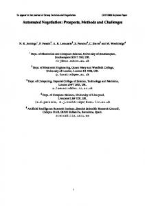
2.2 Attribute Planning This component (whose internal decomposition is shown in Fig. 1) determines the attribute values for the next bid, in such a way that the next bid will always have the target utility as its utility. This is done in two steps: first a target evaluation is computed per attribute, based on the target evaluation planned for the whole bid. Next, attribute values are chosen with the evaluation closest to the target evaluations (for all attributes except price). The configuration of the next bid is then completed by selecting a value for price, such that the utility of the final bid fits exactly its target. In order to make better directed concessions, in planning the target evaluation for each attribute we take into account
not only the own preference weight of the agent, but also the weight of the opponent. If the opponent is not willing to reveal her preference weight for some (or maybe all) attributes, an estimation of these weights is computed in “Estimation of Opponent’s Parameters” component. The role of the “Guess Coefficients” component is to analyze the way the opponent is bidding and to provide some extra information to be used for estimating these private preference weights. In the following we discuss these components in a separate sections. Attribute Planning
Guess Coefficients
Provision of Initial Guess Information
Estimation of Opponent’s Parameters
Target Evaluation Planning
Configuration Planning
Figure 1: Internal composition of Attribute Planning
2.3 Target Evaluation Planning This component outputs a target evaluation for each attribute in the next bid, based on the bid target value. The target attribute evaluation is determined in two steps. First a basic target attribute evaluation for each attribute is computed as: BTE j = EBS, j + (αj / N) (TU - UBS) In the above formula EBS, j represents the evaluation for attribute j in the agent’s own previous bid, UBS the overall evaluation of the agent’s previous bid, while TU represents the target utility for the next bid (as shown in Section 2.1). The parameter αj is chosen as αj = (1 - w j) (1 - EBS, j), where the first parameter expresses the influence of the user’s own importance factor, while the second factor assures that the target evaluation values remain scaled in the interval between 0 and 1. Parameter N is a normalization factor, defined as: N = Σj w j αj. By this choice we ensure that the following relation always holds: Σj w j BTEj = TU (for a full proof of this property we refer the reader to [4]). The Basic Target Evaluation, however only takes into accounts the own preference weights of the agent. Using only this value would work, but tests showed that it leads to sub-optimal results, since the preferences of the other are not considered in any way when making concessions. To improve on this, the following solution was implemented. For each attribute j ∈ A (where A denotes the set of all attributes) a Preference Difference Coefficient δj is computed as:
δ j = (W other, j - W own,j ) / (W other, j + W own,j ) This coefficient (scaled between -1 and 1) expresses how different the preferences of the two parties for each attribute are. Positive values for δj denote a stronger preference of the negotiation partner for attribute j, while negative values denote a stronger own preference for this attribute. The concession to be made in each attribute j ∈ A depends on a parameter called configuration tolerance, denoted as τj ∈ [-1,1]. The tolerance parameter is chosen to be attribute-specific, in order to better differentiate the amount of concessions between attributes. Therefore, for each attribute j∈A, the configuration tolerance depends on the preference difference coefficient of that attribute, according to the following formula: τj = τgen * (1 + δj) Here the parameter τgen represents the general tolerance, used by the agent for all attributes j. The general tolerance is always chosen between 0 and 0.5 and also gives a measure of how fast the agent is willing to make concessions. Values closer to 0 will denote an agent who is less willing to make concessions, while values closer to 0.5 will denote an agent who is interested to reach a deal quickly. Since δj ∈ [-1,1] the tolerance for any attribute j is scaled between 0 and 2*τgen. Finally, the target evaluation for each attribute j is computed. This is done by taking into account both the basic target attribute evaluation (as described above) and a concession to the attribute evaluation from the previous bid of negotiation partner, as follows: TEj = (1 - τj) BTE j + τj EBO, j Here BTE j is the basic attribute evaluation for attribute j and EBO,j is the evaluation for attribute j from the opponent’s previous bid. From the above formula, one can see that values of the configuration tolerance τj close to 0 signify that mostly the user’s own importance factors are taken into account, while values close to 1 shows that maximum possible concession is made towards the other’s value. And since τj depends directly on δj, it is the difference in preference for each attribute that determines how much concession should be made. Because, in our model both the sum of the agent’s own weights and sum of the opponent’s weights are always scaled to 1, the above mechanism leads to a situation where greater concessions in some attributes (more important to the opponent) will always be balanced by smaller concessions in other attributes (more important to me). Such an asymmetric concession system allows both negotiating parties to reach greater utility quicker. In this component we have assumed that the opponent’s preference weights for an attribute are known. However, if the other is not willing to share his weights for some (or all) attributes, then they will need to be estimated.
2.4 Estimation of Opponent’s Parameters This component determines, for those attributes for which the opponent was not willing to reveal his preference
weights, an estimation of those weights. We denote by Aknown the set of attributes for which the opponent was willing to reveal his importance weights in the beginning of the negotiation and by Aunknown the attributes whose preference weights are kept private. Since all preference weights are normalised (see Section 2.1), the sum of weights for the private attributes is computed as: Σj∈Aunknown W j = 1 - Σk∈Aknown W k For attributes with private weights, the remaining weight Σj∈AunknownW j has to be divided between them. For this purpose we assign a parameter called the Remaining Weight Distribution Coefficient Rj to each attribute j ∈ Aunknown. These attributes can be further classified into two subsets: • Attributes for which a reliable guess about the preference of the opponent can be made based on her previous bids (we denote this class by A(G)). These attributes will be assigned a coefficient Rj in the “Guess Coefficients” component (as described in Section 2.5). • Attributes for which no reliable information about the preference weights of the opponent can be made from his previous bids (denoted by A(NG)). These attributes are assigned a default value Rj = 2, which is empirically chosen between the values for attributes for which there is an indication they are important to the opponent (from her past bids) and those attributes which are less important to her (see Table 1). After establishing the value of this parameter, the estimation of the actual weight is computed as follows: Wj = (Rj / Σk∈Aunkown Rk )* Σk∈Aknown W k It is also possible that no reliable information can be obtained from the opponent's past bids for any of the attributes. Then all distribution coefficients will be equal and applying the above formula results in equal distribution of the remaining weight between private attributes, formally expressed as: Aunknown = A(NG) => ∀ j, k ∈ Aunknown, Wj = Wk.
2.5 Guess Coefficients This component analyses the opponent’s bids and, for those attributes for which a trend is reliable detected, returns a value for the remaining weigh distribution coefficient. In the current model the explicit assumption used in guessing (for the Seller's side only) is that, everything else being equal, a human Buyer would prefer a better quality item to a poorer quality one. Otherwise stated there exists a (partial) ordering of the attribute values such as: evaluation(good) > evaluation(fairly good) > evaluation( standard) > evaluation(meager) > evaluation(none). We define the Attribute Value Distance AVTj for each attribute j∈A as the distance between values for an attribute in two successive bids, on an ordinal scale. For example, given the above ordering, the distance between good and fairly good is 1, while the difference between good and standard is 2. It is important to show that this attribute value distance does NOT depend on the exact values the opponent assigns to these labels – since in the current model this information is
private (not disclosed to the other). After running a considerable number of experiments we observed that such a simple ordering information can lead to a reasonably good heuristic. Partial ordering information is usually sufficient to make a good prediction about the opponent's preferences in the negotiation (i.e. if this distance is known only for some labels, this is enough). Next we need a mapping of the detected concession distances to the remaining weight distribution coefficients introduced in Section 2.4 (see Table 1). The values for the above coefficients were determined experimentally as follows: first between each two different labels (representing quality levels) an initial value was computed by subtracting their distance value from 4 (the maximum distance). Then the parameters were adjusted to provide a best linear fit for the results over a large number of tests. This mapping is domain-specific, meaning it lead to good results in the tests we performed, but it may need to be adapted in other domains. Table 1: Remaining Weight Distribution Coefficients assigned to Attribute Value Distances for attrib. j∈ ∈ A(G) Attribute Value Distance(j) 0 1 2 3 4
R (j) 6 4 3 1 0.5
Another issue to be discussed is how many successive bids in the negotiation trace need to be analyzed in order to make a prediction for Rj. From our empirical tests we observed that in most cases it is sufficient to adjust the Rj parameter based only on the first 3 bids. This can be explained by the fact that our model, being cooperative, agreement over the attributes with discrete values occurs in the first rounds of the negotiation – and usually the last rounds can be characterized as “haggling” over the only continuous attribute, the price.
3. EXPERIMENTAL RESULTS In this section, we first discuss the experimental set-up used in testing the proposed model. Then, we illustrate the mathematical model presented in section 2 by means of an example, and summarize the full results from our tests.
3.1 Experimental set-up In order to test the robustness of the above model, we considered the following dimensions: • The number of attribute weights revealed • Whether guessing is used or not • The choice for the attribute importance factors • The evaluations for the attribute value levels Since the test space is very large, we considered 3 cases
of asymmetry in preference. The importance factors used are presented in Table 2. Note that these are raw importance factors, which are then normalised to add up to 1, using the formula presented in Section 2.1. The importance factor for price is kept constant in these tests. The reason for this is that price is the only continuous attribute in the current model (i.e. has a continuous function evaluation) and it is difficult to objectively examine the trade-offs between the other 4 attributes with discrete value labels unless the importance factor of the price is the same. Table 2: Importance factors used for Buyer/Seller, for different levels of preference asymmetry Tow Airco Extra CD Price hedge speakers player Fully asymmetric
90/15
90/15
15/90
15/90
300/300
Partially asymmetric
53/53
90/15
15/90
53/53
300/300
Fully symmetric
53/33
53/53
53/53
53/53
300/300
Furthermore, we must check that these results hold for different possible value configurations. Again the search space here is very large, so we must restrict our attention to a few profiles combinations, which are shown in Table 3. We assume a business model in which the Seller prefers to sell the car for a standard price – and not have to install extra accessories, but he is willing to do so in order to sell it. Other choices are possible, but in order to properly test the model the choice for the values must be asymmetrical – meaning the two parties would like different values for each attribute. Otherwise the parties quickly agree on the configuration (since their interests are convergent) and the negotiation reduces to haggling about the price. Table 3: Value levels Good / Fairly Good/ Standard / Meager / None for each of the 4 attributes
Profile 1
Profile 2
BUYER
100 / 85 / 70 / 30 / 0
100 / 70 / 50 / 35 / 0
SELLER
30 / 65 / 80 / 65 / 100
30 / 50 / 70 / 85 / 100
only a small part of the full mathematical model, but we hope it is enough for the reader to understand the rationale behind some of our design choices. The attribute Tow Hedge has the following normalised preference weights (see Table 2): W BUYER, TowHedge = 90 / (90+90+15+15+300) = 0.1764 WSELLER, TowHedge = 15 / (90+90+15+15+300) = 0.0294 From the perspective of the Seller the preference Difference Coefficient for Tow Hedge will be: δ TowHedge = (W Buyer,TH - W Seller,TH) / (W Buyer, TH + W Seller,TH) = (0.1764-0.0294) / (0.1764+0.0294) = 0.714. A positive value close to 1 (as shown in 2.3), indicates this the attribute is more important to the other party (the Buyer). As the general tolerance (for the Seller side) in this case is τgen = 0.3, the attribute specific tolerance will be τTowHedge = τgen * (1 + δTowHedge) = 0.3 * (1+0.714) = 0.514. Since τTowHedge > τgen, a larger concession than average will be made towards the Buyer’s requested value in this attribute. This can be seen in Table 5 as a large concession, in the first round from “none” to “fairly good”. Next we exemplify the guessing of the opponent’s weights discussed in Sections 2.4 and 2.5. We do this only after the first two rounds from the opponent’s bids, though the mechanism is the same for subsequent rounds. The Value Distances and Remaining Weight Distribution Coefficients for the unknown attributes are (see Table 4 for the Buyer’s first 2 bids and 1 for the coefficient mapping): VD(Airco) = VD(good, standard) = 2 => RAirco = 3 VD(CD_player) = VD(Speakers) = VD(good,meager) = 3 => RCD_player = RSpeakers = 1. Since Σj∈Aunknown Wj =1–(15+300)/510=0.235, the estimated weights are: WAIRCO = 3 / (1+1+3) * 0.235 = 0.141 WCD_PLAYER = 1 / (1+1+3) * 0.235 = 0.047 In this case, the estimations produced by the guessing are not far from the true (non-revealed) values of the Buyer: 0.176 for Airco and 0.0294 for CD player. Tables 4 provides the complete trace of this negotiation from the perspective of the Buyer, while Table 5 does the same from that of the Seller. The vertical columns show the bids made by the two parties in successive rounds. Table 4: The negotiation trace: BUYER’s perspective BUYER
3.2 An example negotiation trace In this section, we illustrate the model presented in Section 2 through an example. Here we take the negotiation between a Buyer and Seller with totally asymmetric preferences (see Table 2), where the only information revealed between parties is the normalised weight of 1 attribute (Tow hedge). For accessories, for both Buyer and Seller, profile 1 is used (see Table 3). For this example, we use the perspective of the Seller, which in our case is the party using guessing. For reasons of space, we can illustrate
1
2
3
4
5
Closing
bids price
18000
17450
17968
18047
18083
18083
Tow hedge
good
fairly good
fairly good
fairly good
fairly good
fairly good
standard standard standard standard
standard
airco
good
speakers
good
meager
none
none
none
none
CD player
good
meager
none
none
none
none
1
0.9203
0.9130
0.9094
0.9068
0.9068
0.7407
0.8782
0.8830
0.8864
0.8889
0.8889
utilities Own bid Seller’s bid
Table 5: The negotiation trace: SELLER’s perspective round 1
SELLER
2
3
4
5
accept:5
bids price
16900
18468
18404
18359
18325
18083
Tow hedge
none
fairly good
fairly good
fairly good
fairly good
fairly good
airco
none
standard
standard
standard
standard
standard
speakers
none
none
none
none
none
none
CD player
none
none
none
none
none
none
Own bid
1
0.9378
0.9296
0.9238
0.9195
0.8884
Buyer’s bid
0.3167
0.5932
0.8737
0.8838
0.8884
0.8884
Fig. 3. The irregular, non-convex shape of the Paretoefficient frontier (computed according to [13]) is typical for real-life domains, where some attributes take discrete values and only some are continuous. Furthermore the frontier does not reach the points (0, 1) and (1, 0). This is because in the evaluation of attribute price cut-off intervals are used. For example the Seller expects to make a maximum profit of 20% over the basic price of the car, and assigns a maximum utility of 1 to any value above that (see [4] for a full discussion of this issue).
utilities
Equal Proportion of Potential line
BUYER 1
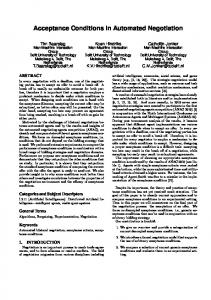
Fig. 2 provides a visualization of the negotiation progress in the joint utility space (as automatically produced by the implementation in our software environment). For clarity, only the first 3 bids of the Buyer and the first 2 of the Seller are shown. The rest lie in the straight line between these 2 points. An interesting effect is that, in this example, after establishing mutually agreeable values for the discrete-value attributes (accesories), the agents seem to “walk” the Paretoefficient frontier towards each other’s bid. This corresponds to the haggling about the price from rounds 3-5 in Tables 4 and 5. BUYER
1
Pareto-efficient frontier
Final agreement point
Pareto-optimal frontier
1-2G
0.9
3NG 1NG
2NG
0 G/NG
0.85
0.8
1
SELLER 3
0.9
0.8
0.85
0.9
1
2
Figure 3: Outcomes for negotiations between a Buyer and Seller with profile 1 and totally asymmetric preference weights
0.8 1
0.7 0.3
0.4
0.5
0.6
0.7
0.8
0.9
1
SELLER
Figure 2: Utility space corresponding to the example trace from Tables 4 and 5
3.3 Comparing traces from the same test set We define a test set as the set of all negotiation traces which share the same Pareto-efficient frontier and therefore whose outcomes are directly comparable. Between the negotiations in the same set the preferences of the two parties are the same: the only difference is the amount of information shared and their willingness to use guessing. In Fig. 3 the final outcomes of negotiations involving a Buyer and Seller with asymmetric preferences and value profile 1 are plotted. The notation is: 1..3 denotes the number of attributes shared and NG/G denotes whether guessing is used or not. The Pareto frontier in Fig. 3 is the same as in fig. 2, just scaled between different values. In fact, the outcome reached in Fig. 2 appears as point 1G in
From the above test set we can already draw some conclusions. First, more attribute weights shared improves the outcome, so the mechanism is able to make efficient use of incomplete preference information. Second, the guessing heuristic may considerably improve the outcome. In the trace presented for 1 or 2 attribute weights shared guessing helps bring the outcome very close to the Pareto-efficient frontier. For 0 attribute weights shared (i.e. perfectly closed negotiation), in this particular test set guessing does not help much (however there are test sets where it does). In the 3 attribute weights shared case the outcome without guessing is already Pareto-efficient. Note however that this case is not equivalent to fully open negotiation, because the evaluations for the values assigned to each quality level are still not revealed between parties.
3.4 Comparing results from all test sets As we showed in Section 3.1, 96 negotiation traces were generated in order to test the validity of our model. Due to
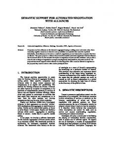
space limitation we cannot present in this paper all our experimental results (the interested reader is asked to consult [14]). In Figure 4 we show the average utilities across the tested profiles, grouped by the level of asymmetry in preference weight between parties. Within each group, from left to right the level of openess is varied from no attributes revealed and no guessing used to 3 attribute weights revealed.
each attribute may differ widely. This ensures that, if the negotiation outcome lies on, or close to, the Pareto-efficient frontier, it will also be relatively close to the KalaiSmorodinsky bargaining outcome. This may be important, since some sources (e.g. [13]) consider closeness to this point as a measure of “fairness” of the negotiation outcome.
4. DISCUSSION
0NG
0,94
0G 1NG
0,92
1G 0,9
2NG 2G
0,88
3NG/G 0,86
0,84
0,82
0,8 Part ially
Fully
Part ially
Fully
asymmet ric
asymmet r ic
asymet ric
asymmet ric
(Buyer )
( Buyer)
(Seller)
(Seller )
Figure 4: Average utilities for all profiles tested, for different cases of preference asymmetry and openess
Based on Figure 4, we can see that our observations from section 3.3 generalize across profiles: both sharing more information and guessing improves the utility (on average). However we found that the more asymmetrical the preferences of the two parties are, the greater the scope for potential gains that can be obtained either by sharing more information or using the guessing heuristic (which can also be seen as the differences between preference configuration groups in Figure 4). For example, for all profile combinations tested in the perfectly symmetrical preferences case, the outcome always had a 0% improvement, either from sharing more preference weight information or by using the guessing heuristic. By contrast in the partially symmetric preferences improvements were of the order of 34%, which went up to around 10% for asymmetric preference weights. This effect can be explained by the fact that our mechanism exploits precisely this preference asymmetry in order to increase the efficiency of the joint outcome for both parties. Another important conclusion is that, if the negotiation speed (see Section 2.1) is set the same for both parties, the outcomes will always lie relatively close to the equal proportion of potential line, regardless of the guessing/openness model used. Otherwise stated, the overall concession for the bid level are similar, even though for
In this section we provide an overview existing work on negotiation, and, by comparison, we discuss different aspects from our own model. In [7], a model for bilateral multi-attribute negotiation is presented, where attributes are negotiated sequentially. The issue studied is the optimal agenda for such a negotiation under both incomplete information and time constraints. However a central mediator is used and the issues all have continuous values. The effect of time on the negotiation equilibrium is the main feature studied, from both a gametheoretic and empirical perspective. In earlier research [8] a slightly different model is proposed, but the focus of the research is still on time constraints and the effect of deadlines on the agents’ strategies. This contrast with our model, where efficiency of the outcome and not time is the main issue studied. This is because we found that, due to our cooperative assumption, a deal is usually reached in maximum 10-15 steps, if the negotiation speed and tolerance parameters are suitably calibrated (see 2.1 & 2.3). The argumentation approach to negotiation (see for e.g. [11] for an overview) allows the agents to exchange not only bids, but also arguments that influence other agents’ beliefs and goals, which, it is claimed, allows more flexibility. Some issues which are usually left open in such approaches are: how do the agents’ mental states relate to their utilities and if (or how) can the efficiency of such negotiations be measured from game-theoretic perspective. Another important direction in multi-attribute negotiations is presented by [9] and [17], which propose models that overcome the linear independence assumption between attribute evaluations. We acknowledge that this is a limitation of the present model, which will be addressed in future work. On the other hand, our model is more flexible in specifying attribute values and better explainable (which may be important for deployment in real domains). For example, both [9] and [17] deal with negotiations only over binary-valued attributes. Furthermore, a simulated annealing approach, such as the one used in [9], although efficient, is computationally rather complex and its results may be difficult to understand intuitively. We also feel that negotiation models which assume independence between attribute evaluations may prove to have other advantages which make them suitable for real e-commerce applications. To make a parallel with machine learning, a simple method such as Naïve Bayes (which also makes an attribute independence assumption) continues to be very widely used in practical applications, despite the advent of more complex
approaches such as neural networks, which avoid this assumption (and are therefore theoretically more “general”). We feel that the most related work to ours is represented by [5] and [6]. Like [5] we start from the perspective of distributed negotiation, which eliminates the need of a central planner. As in [5], we also take the heuristic approach and we model agents that are able to jointly explore the space of possible outcomes with a limited (incomplete) information assumption. In [5], this is done through a trade-off mechanism, in which the agent selects the value of its next offer based on a similarity degree with previous bids of the opponent. In our design, we do no explicitly model trade-offs, yet the same effect is achieved through the asymmetric concessions mechanism. An advantage of our model over [5] is that we allow agents to take into account not only their own weights, but also those of the opponent in order to compute the next bid. In this way agents may exchange partial preference information for those attributes for which their owners feel this does not violate their privacy. Also the initial domain information for the attributes with discrete (“qualitative”) evaluation is different. In [5], this consists of fuzzy value labels, while in our model it is a partial ordering of attribute weights. Our mechanism prevents obvious ways of cheating, like over-stating attribute preference weights. This is because each agent scales the sum of the preference weights declared by the opponent to 1. So an agent has no incentive to overstate his preferences for any attribute, since this may lead to the opponent making smaller or no concessions in other attributes. Furthermore, a system was added by which an agent stops negotiating when it detects insufficient concessions from the other in several successive bids, which should prevent situations where one party makes all the concessions. However, in designing any distributed mechanism, the problem of proving its incentive compatibility remains a challenging one ([3]). A formal proof of the truth-revelation properties of our negotiation protocol was outside the scope of this work. A practical alternative to formal proofs for such designs may be the experimental economics approach (also put forward in [2]). This involves testing the system with a large number of humans (in our case 74 students), negotiating both against software agents and against each other. This part of our research is under submission and still ongoing, but so far we found no obvious ways in which humans can exploit the system in one run.
Acknowledgements: The authors wish to thank Jan Treur (Vrije Universiteit, Amsterdam) for his support during various stages of this research, Lourens van der Meij, scientific programmer at the VU for his aid with the DESIRE implementation and Enrico Gerding and Pieter Jan ‘t Hoen (CWI, Amsterdam) for many useful discussions.
5.REFERENCES [1] Brazier, F.M.T., Jonker, C.M., and Treur, J. “Compositional Design and Reuse of a Generic Agent Model”, Applied Artificial Intelligence Journal, vol. 14, 2000, pp. 491-538. [2] Byde, A., Kay-Yut Chen – “AutONA: A System for Automated Multiple 1-1 Negotiation”, Fourth ACM Conference on Electronic Commerce, pp. 198-199. [3] Dash R. K., Parkes D. C. and Jennings N. R. "Computational Mechanism Design: A Call to Arms" IEEE Intelligent Systems, 2003, vol. 18 (6), pp. 40-47. [4] Jonker, C.M., Treur, J., “An Agent Architecture for MultiAttribute Negotiation”. In: B. Nebel (ed.), Proceedings of the 17th International Joint Conference on AI, IJCAI'01, 2001, pp. 1195 - 1201. [5] Faratin, P., Sierra, C. and Jennings, N. “Using Similarity Criteria to Make Issue Trade-offs in Automated Negotiations”. In Journal of Artificial Intelligence vol. 142 (2), 2003, pp. 205-237. [6] Faratin, P., Sierra, C. and Jennings, N. “Using Similarity Criteria to Make Negotiation Trade-Offs”, Proceedings of ICMAS-2000, Boston, MA., 119-126. [7] Fatima, S. S., Wooldridge, M. and Jennings, N. R.. “Optimal Agendas for Multi-Issue Negotiation”. In Proceedings of the Second International Conference on Autonomous Agents and Multiagent Systems (AAMAS-03), Melbourne, July 2003, pp. 129-136. [8] Fatima, S., Wooldridge, M. and Jennings, N. R.. “Optimal Negotiation Strategies for Agents with Incomplete Information” . In Intelligent Agents VIII, Springer-Verlag LNAI, vol. 2333, pp 377-392, March 2002 [9] Klein, M., Faratin, P., Sayama, H., Bar-Yam, Y “Protocols for Negotiating Complex Contracts”. IEEE Intelligent Systems Journal, special issue on Agents and Markets., vol. 18(6), 2003, pp. 32-38. [10] Gutman, R., Maes, P. – “Agent-mediated Integrative Negotiation for Retail Electronic Commerce”. In P. Noriega and C. Sierra, editors “Agent Mediated Electronic Commerce”, vol 1571 of Lecture Notes in AI, 1998, pp.70-90. [11] Rahwan, I., Ramchurn, S. D. Jennings, N. R., McBurney P., Parsons, S., and Sonenberg L. "Argumentation-based negotiation" Knowledge Engineering Review, to appear 2004. [12] Raiffa, H. – “The art and science of negotiation”, Harvard University Press, Cambridge, Mass., 1982. [13] Raiffa, H. – “Lectures on negotiation analysis”, PON Books, Harvard Law School, 1996. [14] Robu, V. “Improving the efficiency of cooperative negotiations in electronic environments with incomplete information”, Master Thesis, Vrije Univ, Amst., 2003. [15] Rosenschein J. S., Zlotkin G. “Rules of Encounter”, MIT Press, Cambridge, Massachussets, 1994. [16] Strobel, M. “Effects of Electronic Markets on Negotiation Processes”, IBM Research Technical Report, Zurich, 2000. [17] Somefun K., Gerding E., Bohte S. and La Poutré, H. “Automated Negotiation and Bundling of Information Goods”, in Agent-Mediated Electronic Commerce V, Melbourne, Australia, July, 2003.