timizer for comparing between physical design alternatives. Although it provides .... sions to basic INUM that are essential for handling the full complexity of cost ...
Efficient Use of the Query Optimizer for Automated Physical Design †
Stratos Papadomanolakis †
†
Debabrata Dash
†‡∗
Anastasia Ailamaki
‡
Carnegie Mellon University Ecole Polytechnique Fed de Lausanne ´ erale ´ {stratos,ddash,natassa}@cs.cmu.edu
ABSTRACT State-of-the-art database design tools rely on the query optimizer for comparing between physical design alternatives. Although it provides an appropriate cost model for physical design, query optimization is a computationally expensive process. The significant time consumed by optimizer invocations poses serious performance limitations for physical design tools, causing long running times, especially for large problem instances. So far it has been impossible to remove query optimization overhead without sacrificing cost estimation precision. Inaccuracies in query cost estimation are detrimental to the quality of physical design algorithms, as they increase the chances of “missing” good designs and consequently selecting sub-optimal ones. Precision loss and the resulting reduction in solution quality is particularly undesirable and it is the reason the query optimizer is used in the first place. In this paper we eliminate the tradeoff between query cost estimation accuracy and performance. We introduce the INdex Usage Model (INUM), a cost estimation technique that returns the same values that would have been returned by the optimizer, while being three orders of magnitude faster. Integrating INUM with existing index selection algorithms dramatically improves their running times without precision compromises.
1.
INTRODUCTION
As database applications become more sophisticated and human time becomes increasingly expensive, algorithms for automated design and performance tuning for databases are rapidly gaining importance. A database design tool must select a set of design objects (e.g. indexes, materialized views, table partitions) that minimizes the execution time for an input workload while satisfying constraints on parameters such as available storage or update performance. Design tasks typically translate to difficult optimization problems ∗Work done while author was at Carnegie Mellon University.
Permission to copy without fee all or part of this material is granted provided that the copies are not made or distributed for direct commercial advantage, the VLDB copyright notice and the title of the publication and its date appear, and notice is given that copying is by permission of the Very Large Data Base Endowment. To copy otherwise, or to republish, to post on servers or to redistribute to lists, requires a fee and/or special permission from the publisher, ACM. VLDB ‘07, September 23-28, 2007, Vienna, Austria. Copyright 2007 VLDB Endowment, ACM 978-1-59593-649-3/07/09.
Figure 1: Database design tool architecture.
for which no efficient exact algorithms exist [5] and therefore current state-of-the-art design tools employ heuristics to search the design space. Such heuristics trade accuracy for performance by pruning possible designs early without spending time evaluating them. Recent trends, however, dictate that application schemas become richer and workloads become larger – which increases the danger of compromising too much accuracy for the sake of performance. Automated data management cannot rely entirely on aggressive pruning techniques anymore to remain efficient; we need a way to efficiently evaluate large portions of the design space without compromising accuracy and with acceptable performance.
1.1
Accuracy vs. efficiency
Figure 1 outlines the two-stage approach typically employed by database design tools [1, 6, 10, 17]. The candidate selection stage has the task of identifying a small subset of “promising” objects, the Candidates, that are expected to provide the highest performance improvement. The enumeration stage processes the candidates and selects a subset that optimizes workload performance while satisfying given resource constraints. Although tools differ in how they implement Figure 1’s architecture, they all critically rely on the query optimizer for comparing different candidates, because it provides accurate estimates of query execution times. The downside of relying on the optimizer is that query optimization is extremely time-consuming. State-of-the-art tools spend most of their time optimizing queries instead of evaluating as many of the “promising” candidates or candidate subsets as possible. Quoting from a recent study [3]: “...we would require hundreds of optimizer’s calls per iteration, which becomes
1093
prohibitively expensive”. Indeed, our experiments show that on average 90% of the running time of an index selection algorithm is spent in the query optimizer.
1.2
three orders of magnitude faster cost estimation. When factoring in the precomputation phase that involves the optimizer, we measured execution time improvements of 1.3x to 4x – without implementing any of the techniques proposed in the literature for optimizing the number of cost estimation calls, which would result in even higher speedup for INUM. From a different point of view, faster index selection can also be translated to that, given a time limit, an INUMenabled tool can evaluate a wider design space than an optimizer-based tool.
Our approach
This paper presents the INdex Usage Model (INUM), a novel technique for deriving query cost estimates that reconciles the seemingly contradictory goals of high performance and estimation accuracy. INUM is based on the intuition that, although design tools consider an immense space of different of alternative designs, the number of different optimal query execution plans and therefore the number of different possible optimizer outputs is much lower. Thus, it makes sense to cache and reuse the set of plans output by the optimizer, instead of performing multiple invocations only to compute the same plan multiple times. Like the optimizer-based approaches, INUM takes as input a query and a physical design (a set of indexes) and produces as output an estimate for the query cost under the input physical design. Unlike the optimizer-based approaches, however, INUM returns the same value that would have been returned by an equivalent optimizer invocation, without actually performing that invocation. As a consequence from drastically decreasing the dominant overhead of query optimization, INUM allows automated design tools to execute 1.3 to 4 times faster without sacrificing precision.
1.3
Relationship to previous work
There are other studies that have recognized the importance of the accuracy vs. efficiency tradeoff and have designed solutions that follow the cache-and-reuse principle. Recently proposed approaches [3, 4] compute the cost of a query Q for a set of indexes C1 (called a “configuration” [1]), by “locally modifying” the plan generated by the optimizer for another configuration C2 . The plan generated for C2 , however, is not necessarily the optimal plan for C1 , as the indexes in C1 might enable the use of different, more efficient join orders or join algorithms. Therefore, the techniques proposed in [3, 4] compute upper bounds and not the actual query costs, thereby avoiding optimizer calls at the cost of sacrificing accuracy. Using upper bounds instead of actual cost leads to underestimating the “benefit” of configurations and is likely to result in disregarding useful designs. This paper extends the previous work by showing how to apply the cache-and-reuse principle of [3,4] while still deriving accurate cost estimates. We develop a novel framework for matching configurations to their corresponding optimal plans, instead of simply reusing sub-optimal plans. Our primary consideration in this paper is to guarantee that its output is equal to the optimizer’s output when presented with the same input. We describe our technique to accurately and efficiently estimate costs for physical design in the context of index selection algorithms; our approach, however, is also applicable to other physical design features (e.g. materialized views, table partitions) with modifications which are left for future work.
1.4
2. Improved solution quality. INUM allows existing search algorithms (such as greedy search [1, 6]) to examine three orders of magnitude more candidates. Evaluating more candidates benefits solution quality because it reduces the number of “promising” candidates that are overlooked as a result of pruning. According to our experiments, INUM evaluates a candidate set of more than a hundred thousand indexes for a TPC-H based workload, performing the equivalent of millions of optimizer invocations within four hours – a prohibitively expensive task for existing optimizer-based tools. The solution derived from this “power” test improves the solution given by a commercial tool by 20%-30% for “constrained” problem instances with limited storage available for indexes.
Contributions
This paper’s contribution to automated index selection algorithms is as follows: 1. Faster index selection. Our experiments demonstrate that an index selection algorithm with INUM provides
3. 100% Compatibility with existing index selection tools. INUM can be directly integrated into existing tools and database systems, because it simply provides a cost estimation interface without any further assumptions about the algorithm used by the tool. 4. Improved flexibility and performance for new index selection algorithms. Recent work on index selection improves solution quality by dynamically generating candidates, based on a set of transformations and partial enumeration results. The relaxation-based search in [3] generates thousands of new candidates combinations, thereby making optimizer evaluation prohibitively expensive. INUM could help by replacing the approximation logic currently used [3], allowing the algorithm to use exact query costs (as opposed to upper bounds) thereby avoiding estimation errors and the corresponding quality degradation. We propose a novel database design approach, closely integrated with the INUM, elsewhere [13]. The rest of the paper is organized as follows: Sections 2 and 3 present the foundation for the Index Usage Model. Sections 4 and 5 describe our algorithms for caching and reusing query execution plans. Section 6 presents the extensions to basic INUM that are essential for handling the full complexity of cost estimation. Sections 7 and 8 present our experimental results, Section 9 reviews the related work and Section 10 concludes the paper.
2.
INUM FUNDAMENTALS
We show, through an example, how the INUM accurately computes query costs while at the same time eliminating all (but one) optimizer calls. For this section only, we make certain restrictive assumptions on the indexes input to the INUM. This section sets the stage for the complete description of the INUM in the next sections.
1094
2.1
Setup: The Index Selection Session
Consider an index selection session with a tool having the architecture of Figure 1. The tool takes as input a query workload W and a storage constraint, and produces an appropriate set of indexes. We will look at the session from the perspective of a single query Q in W . Let Q be a selectproject-join query accessing 3 tables (T1 , T2 , T3 ). Each table has a join column ID, on which it is joined with the other tables. In addition, each table has a set of 4 attributes (aT1 , bT1 , cT1 , dT1 , etc.) on which Q has numerical predicates of the form x ≤ aTi ≤ y. The automated design tool generates calls to the optimizer requesting the evaluation of Q with respect to some index configuration C. For the remainder of this paper we use the term “configuration” to denote a set of indexes, according to the terminology in previous studies [6]. To facilitate the example presented in this section, we assume that the configurations submitted by the tool to the optimizer contain only non-join columns. No index in any configuration contains any of the ID columns and the database does not contain clustered indexes on ID columns. This is an artificial restriction, used to facilitate the example in this section only. We assume that queries use at most one index per table. For this example, the configurations submitted on behalf of query Q are represented as tuples (T1 : IT1 , T2 : IT2 , T3 : IT3 ), where any of the ITi variables can be empty. Our techniques naturally extend to index unions or intersections, however we maintain the single access method per table throughout the paper, for simplicity 1 . The optimizer returns the optimal query execution plan for Q, the indexes in C utilized by the plan and the estimated cost, along with costs and statistics for all the intermediate plan operators (Figure 2 (a) shows an example optimal query plan). There will be multiple optimizer calls for query Q, one per configuration examined by the tool. Ideally we would like to examine a large number of configurations, to make sure that no “important” indexes are overlooked. However, optimizer latencies in the order of hundreds of milliseconds make evaluating large numbers of configurations prohibitively expensive. Existing tools employ pruning heuristics or approximations to reduce the number of optimizer evaluations. In the next sections we show how to obtain accurate query cost estimates efficiently, with minimal optimization overhead.
2.2
Reasoning About Optimizer Output
Assume we have already performed a single optimizer call for query Q and a configuration C1 and obtained an optimal plan p1 . We first specify the procedure for reusing the information in plan p1 , in order to compute Q’s cost for another configuration C2 . The optimality of plan p1 with respect to configuration C2 is discussed later. To compute the cost of Q under a new configuration C2 , we first compute the internal subplan ip1 from p1 . The internal subplan is the part of the plan that remains after subtracting all the operators relevant to data access (table scans, index scans, index seeks and RID lookups). The internal structure of the plan (e.g. join order and join operators, 1 Our technique only needs to characterize each index by its access cost and the ordering it provides. Both properties can be computed for sets of indexes combined through a union or intersection operator.
Figure 2: Illustration of plan reuse. (a) The optimal plan p1 for configuration C1 . (b) The cost for C2 is computed by reusing the cached internal nodes of plan p1 and adding the costs of the new index access operators, under the assumptions of Section 2.
sort and aggregation operators) remains unchanged. Next, for every table Ti , we construct the appropriate data access operator (index scan or seek with RID lookup) for the corresponding index in C2 (or a table scan operator if the index does not exist). The data access operators are appended to ip1 in the appropriate position. Finally, Q’s cost under C2 can be computed by adding the total cost for ip1 (which is provided by the optimizer) to the cost of the new data access operators corresponding to the indexes in C2 . Given p1 and a new configuration C2 , replacing the optimizer call by the above reuse procedure allows for dramatically faster query cost estimation. Since we have already computed plan p1 (optimal for C1 ), most of the work is already done. The only additional cost is computing the costs of the data access operators in the third step of the reuse procedure: this can be done efficiently and precisely by invoking only the relevant optimizer cost models, without necessitating a full-blown optimization. The reuse procedure is more efficient than an optimizer call because it avoids the overhead of determining a new optimal plan. Figure 2 (b) shows how plan p1 is reused with a new configuration C2 and the new query cost. Since our goal is to maintain accuracy, we must also consider the correctness of reusing a plan p with some input configuration. For our example, reusing plan p1 for C2 will yield erroneous results if the subplan ip1 is not optimal for C2 . In other words, before we reuse plan p for some configuration C we must be in a position to prove that p is optimal for C and this without invoking the optimizer! Focusing on correctness is the differentiating factor between our approach and existing techniques based on “local plan modifications” [3, 4]. The latter do not consider plan optimality and therefore only guarantee the computation of an upper bound for query costs. We now present a correctness proof, based on simple reasoning about optimizer operation. Specifically, for the scenario of this section, we prove that there exists a single optimal subplan for Q, regardless of the configuration C2 , as long as the non-join column constraint of Section 2.1 is satisfied. Since p1 is computed by the optimizer, it has to be
1095
Figure 3: (a) Cost estimation with INUM for the example of Section 2. (b) Complete INUM architecture. the optimal plan and thus it can be safely reused according to our reuse procedure. We intuitively justify this argument by considering how the indexes in C2 affect the query plan cost: Without the join column, there is no reason for C2 to “favor” a particular join order or join algorithm, other than those in p1 . Since the indexes in C2 are not more “powerful” than those in C1 , there is no reason for p1 to stop being optimal. Notice that the non-join column restriction is critical: if it is violated, the reuse procedure will yield incorrect results. We formalize using the following theorem: Theorem 2.1. For a query Q, there is a single optimal plan for all the configurations that do not contain indexes on Q’s join attributes. Proof. We prove Theorem 2.1 by contradiction. Let plans p1 and p2 be optimal plans for configurations C1 and C2 respectively and let p1 , p2 differ in their internal nodes (different join order, for instance). Let ip1 and ip2 be the internal subplans of p1 , p2 and cip1 , cip2 their total costs, with cip1 < cip2 . We first show that the cost of accessing the indexes in C1 and C2 is independent of the internal structure of the plan chosen. Since the join attributes are not indexed, any operator in ip1 and ip2 will scan its corresponding index (or table) with an optional RID lookup. The cost of the scan depends only on the columns of the index and the selectivities of relevant query predicates and is the same regardless of the plan. Thus the index access costs for the indexes in C1 and C2 are the same for plans p1 and p2 . Next, we show that the internal subplans ip1 and ip2 can be used with the indexes of both C1 and C2 (according to the reuse procedure) and that their costs will be the same: Since we assume no join columns, there is no reason why ip1 cannot use the indexes in C2 and vice-versa. In addition, since C1 , C2 do not involve join orders, the only other way a data access operator can affect the internal subplan is through the size and the cardinality of its output, which is the same regardless of the access method used. Thus ip1 and ip2 can use the indexes in C1 and C2 interchangeably and the index access costs and internal plan costs remain the same. Since cip1 < cip2 and the index access costs are the same, using ip1 for C2 is cheaper than using ip2 , and thus p2 is not the optimal plan for C2 . A contradiction.
Theorem 2.1 means that only a single call is sufficient to efficiently estimate Q0 s cost for any configuration, under the no-join column restriction. Our result can be generalized using the notion of an interesting order: Definition 2.1. An interesting order is a tuple ordering specified by the columns in a query’s join, group-by or orderby clause [16]. Definition 2.2. An index covers an interesting order if it is sorted according to that interesting order. A configuration covers an interesting order if it contains an index that covers that interesting order. Although we used a select-project-join query to derive Theorem 2.1, the same reasoning could be applied to queries involving group-by or order-by clauses. For a query with joins, group-by or order-by clauses, only a single plan (and a single optimizer call!) is sufficient to estimate its cost, for all the configurations that do not cover the query’s interesting orders. Figure 3 (a) shows the cost estimation architecture for the restricted tuning session of this section. For every query there is a setup phase, where the single optimal plan is obtained through an optimizer call with a representative configuration. The representative configuration could contain any set of indexes satisfying the non-join or non-interesting order column restrictions (we could even use an empty configuration). The resulting internal subplan is saved in the INUM Space, which is the set of optimal plans maintained by the INUM. Whenever we need to evaluate the query cost for some input configuration C, we use the Index Access Cost Estimation module to estimate the cost of accessing the indexes in C. The sum of the index access costs for C is added to that of the internal subplan to obtain the final query cost. We assume that the Index Access Cost Estimation module is implemented by interfacing to the corresponding estimation modules of the optimizer. Computing only the individual index access costs is much faster than a full-blown optimizer call and does not affect reuse efficiency. Assuming additional optimizer interfaces does not limit INUM’s flexibility. There are other ways to obtain index access costs, for instance through reverse-engineering the optimizer’s analytical cost models. Our evaluation of the INUM with a commercial query optimizer uses pre-computed index access
1096
costs, which are obtained by invoking the optimizer with simplified, “sample” queries.
3.
INUM OVERVIEW
Unlike the scenario of Section 2, in a real index selection session the “no join column” restriction is invalid, as we would typically consider indexes on join columns. The key difference with the previous section is that the assumptions supporting Theorem 2.1 are not valid and thus there might exist more than one optimal plan for a given query.
enough to amortize the initial effort in obtaining the set of optimal plans, by the huge number of optimizer calls that can be performed almost instantly afterward. INUM formalizes the intuitive idea that if a plan is optimal for some configuration C1 , it might in fact remain optimal for a set of configurations that are “similar” to C1 . We use strict rules to determine the optimality of the reused plans, in the form of a matching logic that efficiently assigns, for each configuration input to INUM, the corresponding optimal plan.
3.2 3.1
Caching Multiple Optimal Plans
Ignoring the applicability of multiple feasible plans (with different join orders and algorithms) as a function of multiple index configurations, results in inaccurate cost estimates. To see why, consider the example query of Section 2 and assume a configuration C1 with indexes on T1 .ID and T2 .ID. The optimal plan for C1 first joins T1 and T2 using a merge join and then joins the result with T3 using a hash join. Now assume a configuration C2 , with indexes on T2 and T3 . Now the merge join between T1 , T2 is only feasible by inserting a sort operator on T1 . Existing approximation techniques [3,4] will perform such insertions, ignoring the fact that indexes on T2 and T3 favor an alternative plan that joins T2 and T3 with a merge join, without requiring additional sort operators. To accommodate multiple optimal plans per query, we introduce the concept of the INUM Space, a set that contains, for each query, a number of alternative execution plans. Each plan in the INUM Space is optimal for one or more possible input configurations. The INUM Space is essentially a “cache”, containing plans that can be correctly reused to derive query costs. To guarantee correctness, we require the two properties defined below. Definition 3.1. The INUM Space for a query Q is a set of internal subplans such that: 1. Each subplan is derived from an optimal plan for some configuration. 2. The INUM Space contains all the subplans with the above property. According to Definition 3.1, the INUM Space will contain the optimal plan for any input configuration. Reusing that optimal plan results in accurate cost estimates without invoking the optimizer. The key intuition of this paper is that during the operation of an index design tool, the range of different plans that could be output by the optimizer will be much smaller than the number of configurations evaluated by the tool. In other words we take advantage of the fact that an index design tool might consider thousands of alternative configurations for a query, but the number of different optimal plans for that query is much lower. For example, plans that construct huge intermediate results will never be optimal and thus are not included in the INUM Space. In addition, the optimality of a plan does not change very easily by changing index configurations, because it is determined by additional parameters such as intermediate result sizes. This paper shows that the degree of plan reuse is high
System Architecture
Figure 3 (b) extends Figure 3 (a) with the modules required to implement the full INUM functionality. The INUM takes as input requests from an index selection tool consisting of a query and a configuration for evaluation. The output is the optimal plan and cost for the query. The INUM Space contains, for each query, the set of plans specified by Definition 3.1. The Precomputation module populates the INUM Space at initialization time, by invoking the optimizer in order to reveal the set of optimal plans that need to be cached per query. When invoking the INUM, the Matching module first maps the input configuration to its corresponding optimal plan and derives the query cost without going to the optimizer, simply by adding the cached cost to the index access costs computed on-the-fly. In the remainder of the paper we develop the INUM in two steps. In the first step we exclude from consideration query plans with nested-loop join operators, while allowing every other operator (including sort-merge and hash joins). We call such allowable plans MHJ plans. Section 6 extends our approach to include all join operators. Our two-step approach is necessary because nested-loop join operators require special treatment.
4.
USING CACHED MHJ PLANS
We derive a formula for the query cost given an index configuration and use it to match an input configuration to its corresponding optimal MHJ plan.
4.1
A Formula for Query Cost
Consider a query Q, an input configuration C containing indexes IT1 ..ITn for tables T1 ..Tn and an MHJ plan p in the INUM Space, not necessarily optimal for C. The reuse procedure of Section 2.2 describes how p is used with the indexes in C. Let cip be the sum of the costs of the operators in the subplan ip and sTi be the index access cost for index ITi . The cost of a query Q when using plan p is given by the following equation: cp = cip + (sT1 + sT2 + ... + sTn ) (1) Equation (1) expresses the cost of any plan p as a “function” of the input configuration C. It essentially distinguishes between the cost of the internal operators of a plan p (the internal-subplan, not necessarily optimal) and the costs of accessing the indexes in C. This distinction is key: An optimizer call spends most of its time computing the cip value. INUM essentially works by correctly reusing cached cip values, which are then combined to sTi values computed on-the-fly. The following conditions are necessary for the validity of Equation (1).
1097
1. cip is independent of the sTi ’s. If cip depends on some sTi , then Equation (1) is not linear. 2. The sTi ’s must be independent of p. Otherwise, although the addition is still valid, Equation (1) is not a function of the sTi variables. 3. C must provide the orderings assumed by plan p. If a plan expects a specific ordering (for instance, to use with a merge join) but C does not contain an index to cover this ordering, then it is incorrect to combine p with C. We can show that conditions (1) and (2) hold for MHJ plans through the same argument used in the proof of Theorem 2.1. The indexes in C are always accessed in the same way regardless of the plan’s internal structure. Conversely, a plan’s internal operators will have the same costs regardless of the access methods used (as long as condition (3) holds). Note that the last argument does not mean that the selection of the optimal plan is independent of the access methods used. Condition (3) is a constraint imposed for correctness. Equation (1) is invalid if plan p can not use the indexes in C. We define the notion of compatibility as follows: Definition 4.1. A plan is compatible with a configuration and vice-versa if plan p can use the indexes in the configuration without requiring additional operators. Assuming conditions (1)-(3) hold, Equation (1) computes query costs given a plan p and a configuration C. Next, we use Equation (1) to efficiently identify the optimal plan for an input configuration C and to efficiently populate the INUM Space.
4.2
Mapping Configurations to Optimal Plans
We examine two ways to determine which plan, among those stored in the INUM Space, is optimal for a particular input configuration: An exhaustive algorithm and a technique based on identifying a “region of optimality” for each plan.
4.2.1
Exhaustive Search
Consider first the brute-force approach of finding the optimal plan for query Q and configuration C. The exhaustive algorithm iterates over all the MHJ plans in the INUM Space for Q that are compatible with C and uses Equation (1) to compute their costs. The result of the exhaustive algorithm is the plan with the minimum cost. The problem with the above procedure is that Equation (1) computes the total cost of a query plan p if all the indexes in C are used. If some indexes in C are too expensive to access (for example, non-clustered indexes with low selectivity), the optimal plan is likely to be one that does not use those expensive indexes. In other words, we also need to “simulate” the optimizer’s decision to ignore an index. For this, the exhaustive algorithm needs to also search for the optimal plan for all the configurations C 0 ⊂ C and return the one with the overall minimum cost. We call this iteration over C’s subsets atomic subset enumeration. If the INUM Space is constructed according to Definition 3.1, the exhaustive search with atomic subset enumeration is guaranteed to return correct results, but has the disadvantage of iterating over all the plans in the INUM Space and over all the subsets of C. In the next sections we show
Figure 4: The cost functions for MHJ plans form parallel hyper-surfaces. how to avoid the performance problems of the exhaustive search by exploiting the properties of Equation (1).
4.2.2
Regions of Optimality
Consider a query Q accessing 2 tables, T1 and T2 , with attributes {ID, a1 , b1 } and {ID, a2 , b2 }. Q joins T1 and T2 on ID and projects attribute a1 of the result. Let C be a configuration with two indexes, IT1 and IT2 , on attributes {T1 .ID, T1 .a1 , T1 .b1 } and {T2 .ID, T2 .a2 ,T2 .b2 } respectively. Let p1 be a merge join plan that is the optimal MHJ plan for C. We ignore the subset enumeration problem for this example, assuming that we have no reason not to use IT1 and IT2 . What happens if we change C to C1 , by replacing IT1 with IT0 1 : {ID, a1 }? We can show that plan p1 remains optimal and avoid a new optimizer call, using an argument similar to that of Section 2.2. Assume that the optimal plan for C1 is p2 that uses a hash join. Since the index access costs are the same for both plans, by Equation (1) the cip value for p2 must be lower than that for p1 and therefore p1 cannot be optimal for C, which is a contradiction. The intuition is that since both C and C1 are capable of “supporting” exactly the same plans (both providing ordering on the ID columns), a plan p found to be optimal for C must be optimal for C1 and any other configuration covering the same interesting orders. The set O of interesting orders that is covered by both C and C1 is called the region of optimality for plan p. We formalize the above with the following theorem. Theorem 4.1. For all the configurations covering the same set of interesting orders O there exists a single optimal MHJ plan p, such that p accesses all the indexes in a configuration. Proof. Let C(O) be a set of configurations covering the given interesting order O. Also, consider the set P of all the MHJ plans that are compatible with the configurations in C(O). For every configuration C in C(O) containing indexes on tables T1 ,...,Tn we can compute the index access costs sT1 ,...,sTn independently of a specific plan. Conceptually, we map C to an n-dimensional point (sT1 , sT2 , ..., sTn ). The cost function cp for a plan p in P is a linear function of the sTi parameters and corresponds to a hypersurface in the (n+1)-dimensional space formed by the index access cost vector and cp . To find the optimal plan for a configuration C, we need to find the plan hypersurface that gives us the lowest cost value.
1098
Parametric Query Optimization (PQO) techniques [11,12] can be directly applied to piecewise linear cost functions like those in Figure 5, in order to directly find the optimal plan given the index access cost values. We omit the details of a PQO model due to lack of space.
5.
Figure 5: Modified plan comparison taking into account index I/O costs. The optimal plan for expensive indexes (to the right of the thick line) performs a sequential scan and uses a hash join. By the structure of Equation (1) all hypersurfaces are parallel, thus for every configuration in C(O) there exists a single optimal plan. Figure 4 shows the cost hypersurfaces for a merge and a hash join plan, joining tables T1 and T2 . To avoid 2dimensional diagrams, assume we fix the index built on T2 and only compute the plan cost for the indexes on T1 that cover the same interesting order. The optimal plan for an index IT1 corresponds to the hypersurface that first intersects the vertical line starting at the point IT1 . Since the plan cost lines are parallel, the optimal plan is the same for all the indexes regardless of their sTi values. The INUM Space exploits Theorem 4.1 by storing for each plan its region of optimality. The INUM identifies the optimal plan for a configuration C by first computing the set of interesting orders O covered by C. O is then used to find the corresponding plan in the INUM Space. By Theorem 4.1 the retrieved plan will be the optimal plan that accesses all the indexes in C. Like in the case of the exhaustive algorithm, to obtain the globally optimal plan the above procedure must be repeated for every subset C 0 of C.
4.2.3
Atomic Subset Enumeration
To find the query cost for an input configuration C we need to apply Theorem 4.1 for every subset of C and return the plan with the lowest cost. Enumerating C’s subsets for n tables with an indexes for every table requires 2n iterations. Since each “evaluation” corresponds to a fast lookup, the exponent does not hurt performance for reasonable n values. For n = 5, subset enumeration requires merely 32 lookups. The overhead of subset enumeration might be undesirable for queries accessing 10 or 20 tables. For such cases we can avoid the enumeration by predicting when the optimizer will not use an index of the input configuration C, or equivalently use a specific subset C 0 . It can be shown that an index is not used only if it has an access cost that is too high. By storing with each plan the ranges of access costs for which it remains optimal, the INUM can immediately find the indexes that will actually be used. Figure 5 shows an example of how the plan curves of Figure 4 change to incorporate index access costs. The hash join cost flattens after the index access cost exceeds the table scan cost (there is no need to access that index for a hash join plan). The hash join is optimal for indexes in the region to the right of the intersection point between the merge and hash join lines.
COMPUTING THE INUM SPACE
Theorem 4.1 in Section 4.2.2 suggests a straightforward way for computing the INUM Space. Let query Q reference tables T1 , ..., Tn and let Oi be the set of interesting orders for table Ti . We also include the “empty” interesting order in Oi , to account for the indexes on Ti that do not cover an interesting order. The set O = O1 × O2 × ... × On contains all the possible combinations of interesting orders that a configuration can cover. By Theorem 4.1, for every member of O there exists a single optimal MHJ plan. Thus, to compute the INUM Space it is sufficient to invoke the optimizer once for each member o of O, using some representative configuration. The resulting internal subplan is sufficient, according to Theorem 4.1, for computing the query cost for any configuration that covers o. In order to obtain MHJ plans, the optimizer must be invoked with appropriate hints to prevent consideration of nested-loop join algorithms. Optimizer operation is faster during the pre-computation phase because the use of hints reduces the space of alternative plans that must be examined for a query. The precomputation phase requires fewer optimizer calls compared to optimizer-based tools, as the latter deal with different combinations of indexes, even if the combinations cover the same interesting orders. The number of MHJ plans in the INUM Space for a query accessing n tables is |O1 | × |O2 | × ... × |On |. Consider a query joining n tables on the same id attribute. There are 2 possible interesting orders per table, the id order and the empty order that accounts for the rest of the indexes. In this case the size of INUM Space is 2n . For n = 5, 32 optimizer calls are sufficient for subsequently estimating the query cost for any configuration without further optimizer invocation. For larger n, for instance for queries joining 10 or 20 tables, precomputation becomes expensive, as more than a thousand optimizer calls are required to fully compute the INUM Space. Large queries are a problem for optimizerbased tools as well, unless specific measures are taken to artificially restrict the number of atomic configurations examined [6]. Fortunately, there are ways to optimize the performance of INUM construction, so that it still outperforms optimizer-based approaches. The main idea is to evaluate only a subset of O without sacrificing precision. We propose two ways to optimize precomputation, lazy evaluation and cost-based evaluation. Lazy evaluation constructs the INUM Space incrementally, in-sync with the index design tool. Since the popular greedy search approach selects one index at a time, there is no need to consider all the possible combinations of interesting orders for a query up-front. The only way that the full INUM Space is needed is for the tool to evaluate an atomic configuration containing n indexes covering various interesting orders. Existing tools avoid a large number of optimizer calls by not generating atomic configurations of size more than k, where k is some small number (according to [6] setting k = 2 is sufficient). With small-sized atomic configurations, the number of calls that INUM needs is a lot
1099
Figure 6: NLJ plan costs for a single table as a function of an index’s sN L parameter (System R optimizer).
Figure 7: NLJ plan cost curves for a single table and an unknown cost function of a single index parameter sI .
smaller. Cost-based evaluation is based on the observation that not all tables have the same contribution to the query cost. In the common case, most of the cost is due to accessing and joining a few expensive tables. We apply this idea by “ignoring” interesting orders which are unlikely to significantly affect query cost. For a configuration covering an “ignored” order, the INUM will simply return a plan that will not take advantage of that order and thus have a slightly higher cost. Notice that only the cip parameter of Equation (1) is affected and not the sTi ’s. If an index on an “ignored” order has a significant I/O benefit (if for example, it is a covering index) the I/O improvement will still correctly be reflected in the cost value returned by the INUM. Cost-based evaluation is very effective in TPC-H style queries, where it is important to capture efficient plans for joining the fact table with one or two large dimension tables, while the joining of smaller tables is not as important.
tuples in the table. W and RSI account for the CPU costs. It is easy to see that N and RSI are not independent of the plan, since both are determined by the number of qualifying outer tuples. We define the nested loop access cost sN L as sN L = F × (P ages(I) + Card(T )) and set W = 0 for simplicity. The nested-loop cost becomes: cp = cout + N × sN L . Figure 6 shows the cost of different plans as a function of the nested-loop access cost for a single table. The difference with Figure 4 is that the hypersurfaces describing the plan costs are no longer parallel. Therefore for indexes covering the same set of interesting orders there can be more than one optimal plan. In Figure 6, plan p2 gets better than p1 as the sN L value increases, because it performs fewer index lookups. (lower N value and lower slope). The System R optimizer example highlights two problems posed by the NLJ operator. First, it is more difficult to find the entire set of optimal plans because a single optimizer call per interesting order combination is no longer sufficient. For the example of Figure 6, finding all the optimal plans requires at least two calls, using indexes with high and low sN L values. A third call might also be necessary to ensure there is no other optimal plan for some index with an intermediate sN L value. The second problem is that defining regions of optimality for each plan is not as straightforward. The optimality of an NLJ plan is now predicated on the sN L values of the indexes, in addition to the interesting orders they cover. In modern query optimizers, the cost of a nested-loop join operator is computed by more complicated cost models compared to System R. Such models might require more parameters for an index (as opposed to the sN L values used for System R) and might have plan hypersurfaces with a non-linear shape. Determining the set of optimal plans and their regions of optimality requires exact knowledge of the cost models and potentially the use of non-linear parametric query optimization techniques [12]. In this paper we are interested in developing a general solution that is as accurate as possible without making any assumptions about optimizer internals. The development of optimizer-specific models is an interesting area for future research.
6.
EXTENDING THE INUM
In this section we consider plans containing at least one nested-loop join operator in addition to merge or hash join operators. We call such plans NLJ plans. We explain why plans containing nested-loop joins require additional modeling effort and present ways to incorporate NLJ plans in the INUM.
6.1
Modeling NLJ Plans
The cost of an NLJ plan can not be described by Equation (1) of Section 4.1. Therefore we can no longer take advantage of the linearity properties of Equation (1) for determining the plans that must be stored in the INUM Space and characterizing their regions of optimality. We present an example based on System R’s query optimizer [16] to illustrate the special properties of NLJ plans. Note that we do not rely or use System R’s cost model in our system. The techniques in this section are not dependent on particular cost models, rather they capture the general behavior of NLJ plans. The System R example in this section is for illustration purposes only. For System R the cost of a plan using index nested-loop join is expressed by cout + N × cin , where cout is the cost of the outer input, cin is the cost of accessing the inner relation through index I and N is the number of qualifying outer tuples. cin is given by cin = F ×(P ages(I)+Card(T ))+W ×RSI, where F is the selectivity of the relevant index expressions, P ages(I) is the index size and Card(T ) is the number of
6.2
Extending INUM with NLJ Plans
In this section we develop general methods for populating the INUM Space with NLJ plans in addition to MHJ plans and for determining the overall optimal plan given an input configuration. We begin with the problem of obtaining a set of optimal
1100
NLJ plans from the optimizer. We assume that each index is modeled by a single index parameter sI (like the sN L parameter in Section 6.1) that relates to its properties but we do not have access to the precise definition of sI . The formula relating the sI parameters to the plan costs is also unknown. Let Imin and Imax be two indexes having minimum and maximum sI values respectively. We also assume that the plan’s cost function is monotonically increasing, thus every plan has a minimum cost value for the most “efficient” index Imin and maximum cost for Imax . We present our approach using a simple example with a single table and a single interesting order. Figure 7 shows the plan costs for two different NLJ plans, as a function of a single index parameter sI . Even without precise knowledge of the cost functions, we can retrieve at least two plans. Invoking the optimizer with Imin returns plan p1 , while Imax returns plan p2 . There is no way without additional information to identify intermediate plans, but p1 and p2 are a reasonable approximation. Identifying the Imin , Imax indexes for a query is easy: Imin provides the lowest possible cost when accessed through a nested-loop join, thus we set it to be a covering index 2 . Using the same reasoning, we set Imax to be the index containing no attributes other than the join columns. Performing 2 calls, one for Imin and for Imax leads to two possible outcomes: 1. At least one call returns an NLJ plan. There might be more plans for indexes in-between Imax and Imin . To reveal them we need more calls, with additional indexes. Finding those intermediate plans requires additional information on optimizer operation. 2. Both calls return an MHJ plan. If neither Imin nor Imax facilitates an NLJ plan, then no other index covering the same interesting order can facilitate an NLJ plan. In this case, the results of the previous sections on MHJ plans are directly applicable: By Theorem 4.1, the two calls will return the same MHJ plan. For queries accessing more than one table, INUM first considers all interesting order subsets, just like the case with MHJ plans. For a given interesting order subset, there exist an Imin and Imax index per interesting order. The INUM performs an optimizer call for every Imin and Imax combination. This procedure results in more optimizer calls compared to the MHJ case, which required only a single call per interesting order combination. Multiple calls are necessary because every individual combination of Imin and Imax indexes could theoretically generate a different optimal plan. We reduce the number of optimizer calls during NLJ plan enumeration by caching only a single NLJ plan and ignoring the rest. Instead of performing multiple calls for every Imin , Imax combination, the INUM invokes the optimizer only once, using only the Imin indexes. If the call returns an NLJ plan then it gets cached. If not, then INUM assumes that no other NLJ plans exist. The motivation for this heuristic is that a single NLJ plan with a lower cost than the corresponding MHJ plan is sufficient to prevent INUM from overestimating query costs. If such a lower NLJ 2
There exist cases where Imin is a non-covering index, but in this case the difference in costs must be small. Generally, the covering index is a good approximation for Imin .
plan exists, invoking the optimizer using the most efficient indexes (Imin ) is very likely to reveal it. Selecting the optimal plan for an input configuration when the INUM Space contains both MHJ and NLJ plans is simple. The optimal MHJ plan is computed as before (Section 4.2). If the INUM Space also contains an NLJ plan, the index access costs can be computed by the optimizer separately (just like for an MHJ plan) and added to the cached NLJ plan cost. INUM compares the NLJ and MHJ plans and returns the one with the lowest cost.
6.3
Modeling Update Statements
The INUM can readily be extended to estimate the cost of update statements (SQL INSERT, UPDATE and DELETE). An update can be modeled as two sub-statements: The “select” part is the query identifying the rows to be modified and the “modify” part is the actual data update. The former is just another query and can be readily modeled by the INUM. The cost of the latter depends on factors such as the number of updated rows, the row size and the number of structures (indexes, views) that must be maintained. Similarly to the individual index access costs, obtaining the cost of an update operation is simply a matter of interfacing to the relevant optimizer cost modules and involves a simple, inexpensive computation. Note that from a cost estimation perspective, handling updates is simple. The impact of updates on the design algorithms themselves and on their solution quality is an extremely interesting research topic, but beyond the scope of this paper, that focuses only on cost estimation.
7.
EXPERIMENTAL SETUP
We implemented INUM using Java (JDK1.4.0) and interfaced our code to the optimizer of a commercial DBMS, which we will call System1. Our implementation demonstrates the feasibility of our approach in the context of a real commercial optimizer and workloads and allows us to compare directly with existing index selection tools. To evaluate the benefits of INUM, we built on top of it a very simple index selection tool, called eINUM. eINUM is essentially an enumerator, taking as input a set of candidate indexes and performing a simple greedy search, similar to the one used in [6]. We chose not to implement any candidate pruning heuristics because one of our goals is to demonstrate that the high scalability offered by INUM can deal with large candidate sets that have not been pruned in any way. We “feed” eINUM with two different sets of candidate indexes. The exhaustive candidate set is generated by building an index on every possible subset of attributes referenced in the workload. From each subset, we generate multiple indexes, each having a different attribute as prefix. This algorithm generates a set of indexes on all possible attribute subsets, and with every possible attribute as key. The second candidate set, the heuristic, emulates the behavior of existing index selection tools with separate candidate selection modules. We obtain heuristic candidates by running commercial tools and observing all the indexes they examine through tracing. The purpose of the heuristic candidate set is to approximate how INUM would perform if integrated with existing index selection algorithms. Besides the automated physical design tool shipping with System1, we compare eINUM with the design tool of a sec-
1101
Figure 8: Experimental results for TPCH15. (a) Optimizer calls vs. time for an exhaustive candidate set (b) Recommendation quality (c) Optimizer calls vs. time for a heuristic candidate set ond commercial DBMS, System2. We were unable to port eINUM to System2 because it does not allow us to use index hints. Since we never actually ran eINUM with System2’s query optimizer, we cannot report on a direct comparison, but we include System2 results for completeness. Integrating INUM with more commercial and open source database management systems is part of our ongoing work. We experiment with two datasets. The 1GB version of the TPC-H benchmark 3 and the NREF protein database described in [8]. The NREF database consists of 6 tables and consumes 1.5 GBs of disk space. For TPC-H, we used a workload consisting of 15 out of the 22 queries, which we call TPCH15. We were forced to omit certain queries due to limitations in our parser but our sample preserves the complexity of the full workload. The NREF workload consists of 235 queries involving joins between 2 and 3 tables, nested queries and aggregation. We use a dual-Xeon 3.0GHz based server with 4 gigabytes of RAM running Windows Server 2003 (64bit). We report both tuning running times and recommendation quality, that is computed using optimizer estimates. Improvements are computed by: costindexed . %improvement = 1 − cost not indexed
8.
EXPERIMENTAL RESULTS
In this section we demonstrate the superior performance and recommendation quality of eINUM compared to System1 and System2 for our TPCH15 and NREF workloads.
8.1 8.1.1
TPCH15 Results Exhaustive Tuning Performance
We provided eINUM with an exhaustive candidate set for TPCH15 consisting of 117000 indexes. For the exhaustive experiment we ran all the tools without specifying a storage constraint. Figure 8 (a) shows the number of cost estimation calls performed by the 3 systems and the time it took to complete them. The data for the two commercial systems come from traces of database activity. The horizontal axis corresponds to optimization time: for each point in the horizontal axis, the graph shows the number of estimation calls up to that point. The graph focuses only on the tuning time spent during cost estimation and not the overall 3 We chose a relatively small version for TPC-H to speed-up administrative tasks such as building statistics and “real” indexes to validate our results. Dataset size affects the numerical values returned by the cost models but not the accuracy and speed of the INUM.
execution time, which includes the algorithm itself, virtual index construction and other overheads. Query cost estimation dominates the execution time for all cases, so we discuss this first. We report on the additional overheads (including the time to construct the INUM model) later. According to Figure 8 (a), eINUM performs the equivalent of 31 million optimizer (per query) invocations within 12065 seconds (about 3.5 hours), or equivalently, 0.3ms per call. Although such a high number of optimizer invocations might seem excessive for such a small workload, INUM’s ability to support millions of evaluations within a few hours will be invaluable for larger problems. Compare eINUM’s throughput with that of the state-ofthe-art optimizer based approaches (notice that the graph is in logarithmic scale). System1 examines 188 candidates in total and performs 178 calls over 220 seconds, at an average 1.2s per call. System2 is even more conservative, examining 31 candidates and performing 91 calls over 7 seconds at 77ms per call. System2 is faster because it does not use the optimizer during enumeration. However, as we see in the next paragraph, it provides lower quality recommendations. Another way to appreciate the results is the following: If we had interrupted eINUM after 220 seconds of optimization time (the total optimization time of System1, it would have already performed about 2 million evaluations! The construction of the INUM took 1243s, or about 21 minutes, spent in performing 1358 “real” optimizer calls. The number of actual optimizer calls is very small compared to the millions of INUM cost evaluations performed during tuning. Also, note that this number corresponds to an experiment with a huge candidate set. As we show later, we can “compress” the time spent in INUM construction for smaller problems. System1 required 246 seconds of total tuning time: For System1, optimization time accounted for 92% of the total tool running time. System2 needed 3 seconds of additional computation time, for a total of 10 seconds. The optimization time was 70% of the total tuning time.
8.1.2
Exhaustive Tuning Quality
Figure 8 (b) shows the recommendation quality for the three systems under varying storage constraints, where eINUM used the exhaustive candidate set. The percentage improvements are computed over the unindexed database (with only clustered indexes on the primary keys). The last data point for each graph corresponds to a session with no storage constraint. INUM’s recommendations have 8%-34% lower cost compared to those of System1. System2’s unconstrained result was approximately 900MB,
1102
so we could not collect any data points beyond this limit. To obtain the quality results shown in Figure 8 (b), we implemented System2 recommendations in System1 and used System1’s optimizer to derive query costs. The results obtained by this method are only indicative, since System2 is at a disadvantage: It never had the chance to look at cost estimates from System1 during tuning. It performs slightly worse than System1 (and is 37% worse than eINUM but the situation is reversed when we implement System1’s recommendation in System2 (we omit those results). The only safe conclusion to draw from System2 is that it fails to take advantage of additional index storage space. We attribute the superior quality of eINUM’s recommendations is to its larger candidate set. Despite the fact that eINUM is extremely simple algorithmically, it considers candidates that combine high improvements with low storage costs, because they are useful for multiple queries. Those indexes are missed by the commercial tools, due to their restricted candidate set.
8.1.3
Heuristic Enumeration
In this section we demonstrate that using INUM in combination with existing index selection algorithms can result in huge savings in tuning time without losing quality. We use eINUM without a storage constraint and we provide it with a candidate index set consisting of 188 candidate indexes considered by System1. System1 was configured exactly the same way as in the previous session. Figure 8 (c) shows the timing results for eINUM comparing with System1, in a logarithmic plot. eINUM performs more query cost estimation calls (7440 compared to 178), yet cost estimation requires only 1.4 seconds compared to the 220 seconds for System1. For a fair comparison, we must also take into account the time to compute the INUM Space. With lazy precomputation (Section 5), INUM construction took 180.6 seconds. Overall, eINUM took 182 seconds compared to 246 seconds for System1. Note that eINUM does not implement any of the atomic configuration optimizations proposed in the literature for optimizer-based tools [6]. Incorporating additional optimizations would have reduced the precomputation overhead, since it would allow a further reduction in the number of optimizer calls. The quality reached by the two algorithms was the same, which makes sense given that they consider exactly the same candidates.
8.1.4
INUM Precision
INUM’s estimates do not exactly match the query optimizer’s output. Even the optimizer itself, due to various implementation details such as variations in statistics, provides slightly different cost values if called for the same query and the same configurations. These slight differences exist between the plans saved by the INUM and the ones dynamically computed by the optimizer. We measure the discrepancy E between the optimizer estimate for the entire workload cost copt and the INUM estimate cIN U M by E = 1 − cIN U M /copt . We compute E at the end of every pass performed by eINUM over the entire candidate set and we verify that the INUM cost estimate for the solution computed up to that point agrees with the “real” optimizer estimate. We never found E to be higher than 10%, with an average value of 7%. We argue that a 10% error in our estimate is negligible,
Figure 9: Optimizer calls vs. time for the NREF workload
compared to the scalability benefits offered by the INUM. Besides, existing optimizer-based tools that use atomic configuration optimizations [6] or the benefit assignment method for the knapsack formulation [10] already trade accuracy for efficiency.
8.2
NREF Results
In this section, we present our results from applying eINUM with an exhaustive candidate index set on the NREF workload. NREF is different from TPCH15 in that it contains more queries (235) that are simpler in terms of the number of attributes they access: Each query accesses 2 to 3 columns per table. Figure 9 compares eINUM and System1 in terms of the time spent in query cost estimation. eINUM performed 1.2M “calls”, that took 180s (0.2ms per call). System1 performed 952 optimizer calls that took 2700s (or 2.9s per call). INUM construction took 494s (without any performance optimizations whatsoever), while the total time for System1 was 2800s. Interestingly, searching over the exhaustive candidate set with eINUM was about 6 times faster compared to System1, despite the latter’s candidate pruning heuristics. We also compare the recommendation quality for various storage constraints, and find that eINUM and System1 produce identical results. This happens because NREF is easier to index: Both tools converge to similar configurations (with single or two-column indexes) that are optimal for the majority of the queries.
9.
RELATED WORK
They key elements of modern automated database design tools are introduced in [1, 6, 10]. They strongly advocate the tight integration of database design algorithms and the query optimizer, in order to ensure that the recommended designs do in fact reflect the “true” (at least, as perceived by the system) query costs. The INUM, presented in this paper, addresses the downside of relying on query optimization: its large computational overhead and the aggressive heuristics required to minimize it. [5] shows that index selection is a computationally hard problem and thus efficient exact solutions do not exist. Design tools utilize some variation of a greedy search procedure to find a design that satisfies resource constraints and is locally-optimal. An example is the greedy(m, k) heuristic introduced of [1, 6]. Another approach uses a knapsack formulation [10] that greedily selects candidates based on their benefit to storage cost ratio. The knapsack-based approach is extended by [5], where a linear programming tech-
1103
nique is used for accurate weight assignment. [14] applies similar greedy heuristics, along with a genetic programming algorithm, to the design problem of table partitioning in a parallel SQL database. The Index Merging [7] work extends the basic design framework with more sophisticated techniques for performing candidate selection through merging candidate indexes. More recent work [3] suggests combining candidate selection with the actual search, so that the partial search results can be used to generate more useful candidates through various transformations. Both studies highlight the importance of effective candidate selection algorithms, that do not omit “potentially interesting” design candidates. INUM improves algorithms for candidate selection (and the subsequent search) by allowing large candidate spaces to be constructed and traversed efficiently. Modern database design tools support additional design features such as materialized views [1,17], table partitions [2] and multidimensional clustering [17]. Having multiple object types increases the complexity of design algorithms, because combining design features generates very large joint search spaces. INUM can be extended to handle physical design features other than indexes and we expect its performance benefits to be even more pronounced when dealing with larger search spaces. The work on Parametric Query Optimization (PQO) for linear, piece-wise linear and non-linear functions [11,12] studies the change in the optimal plan for a query under changing numerical parameters, such as predicate selectivities. The INUM has the same goal, only that now the changing parameter is the underlying physical design, which cannot be captured solely by numerical values. The PQO framework, however, is invaluable in dealing with complex optimizer cost functions, especially the non-linear ones described in Section 6.1. [15] presents an empirical study of the plan space generated by commercial query optimizers, again under varying selectivities. Their results suggest that while the space of optimal plans determined by the optimizer for a query might be very large, it can be substituted by another containing a smaller number of “core” plans without much loss in quality, an observation very similar to our own (See Section 3). [9] presents a technique to avoid unnecessary optimizer calls, by caching and sharing the same plan among multiple similar queries. They define query similarity based on a number of query features (such as query structure and predicates). Although a clustering approach is conceivable for our problem, it is not clear how to derive the necessary precision guarantees.
10.
CONCLUSION
Index selection algorithms are built around the query optimizer, but query optimization complexity limits their scalability. We introduce INUM, a framework that solves the problem of expensive optimizer calls by caching and efficiently reusing a small number of key optimizer calls. INUM provides accurate cost estimates during the index selection process, without requiring further optimizer invocations. We evaluate INUM in the context of a real commercial query optimizer and show that INUM improves enumeration performance by orders of magnitude. In addition, we demonstrate that being able to evaluate a larger number of candidate indexes through INUM improves recommendation quality.
11.
REFERENCES
[1] Sanjay Agrawal, Surajit Chaudhuri, and Vivek R. Narasayya. Automated selection of materialized views and indexes in SQL databases. In Proceedings of the VLDB Conference, 2000. [2] Sanjay Agrawal, Vivek Narasayya, and Beverly Yang. Integrating vertical and horizontal partitioning into automated physical database design. In Proceedings of the SIGMOD Conference, 2004. [3] Nicolas Bruno and Surajit Chaudhuri. Automatic physical database tuning: a relaxation-based approach. In Proceedings of the SIGMOD Conference, 2005. [4] Nicolas Bruno and Surajit Chaudhuri. To tune or not to tune? a lightweight physical design alerter. In Proceedings of the VLDB Conference, 2006. [5] Surajit Chaudhuri, Mayur Datar, and Vivek Narasayya. Index selection for databases: A hardness study and a principled heuristic solution. IEEE Transactions on Knowledge and Data Engineering, 16(11):1313–1323, 2004. [6] Surajit Chaudhuri and Vivek R. Narasayya. An efficient cost-driven index selection tool for Microsoft SQL server. In Proceedings of the VLDB Conference, 1997. [7] Surajit Chaudhuri and Vivek R. Narasayya. Index merging. In Proceedings of the ICDE Conference, 1999. [8] Mariano P. Consens, Denilson Barbosa, Adrian Teisanu, and Laurent Mignet. Goals and benchmarks for autonomic configuration recommenders. In Proceedings of the SIGMOD Conference, 2005. [9] A. Ghosh, J. Parikh, V. Sengar, and J. Haritsa. Plan selection based on query clustering. In VLDB, 2002. [10] G.Valentin, M.Zuliani, D.Zilio, and G.Lohman. DB2 advisor: An optimizer smart enough to recommend its own indexes. In Proceedings of the ICDE Conference, 2000. [11] Arvind Hulgeri and S. Sudarshan. Parametric query optimization for linear and piecewise linear cost functions. In VLDB, 2002. [12] Arvind Hulgeri and S. Sudarshan. AniPQO: Almost non-intrusive parametric query optimization for nonlinear cost functions. In Proceedings of the VLDB Conference, 2003. [13] Stratos Papadomanolakis and Anastassia Ailamaki. An integer linear programming approach to database design. In ICDE Workshop on Self-Managing Databases, 2007. [14] Jun Rao, Chun Zhang, Nimrod Megiddo, and Guy Lohman. Automating physical database design in a parallel database. In Proceedings of the SIGMOD Conference, 2002. [15] Naveen Reddy and Jayant R. Haritsa. Analyzing plan diagrams of database query optimizers. In Proceedings of VLDB, 2005. [16] P. Selinger, M. Astrahan, D. Chamberlin, R. Lorie, and T. Price. Access path selection in a relational database management system. In SIGMOD 1979. [17] Daniel C. Zilio, Jun Rao, Sam Lightstone, Guy M. Lohman, Adam Storm, Christian Garcia-Arellano, and Scott Fadden. DB2 design advisor: Integrated automatic physical database design. In VLDB, 2004.
1104