use the concepts of Fuzzy Set Theory to automate the process of human ... The applicability of automated ..... MineSetâ¢, data mining software from Silicon Graphics (see. [1]). ..... example, in a marketing survey the records constituting just.
Automated Perceptions in Data Mining Mark Last and Abraham Kandel Department of Computer Science and Engineering University of South Florida 4202 E. Fowler Avenue, ENB 118 Tampa, FL 33620, USA (E-mail: {mlast, kandel}@csee.usf.edu)
Abstract Visualization is known to be one of the most efficient data mining approaches. The human eye can capture complex patterns and relationships, along with detecting the outlying (exceptional) cases in a data set. The main limitation of the visual data analysis is its poor scalability: it is hardly applicable to data sets of high dimensionality. We use the concepts of Fuzzy Set Theory to automate the process of human perception. The automated tasks include comparison of frequency distributions, evaluating reliability of dependent variables, and detecting outliers in noisy data. Multiple perceptions (related to different users) can be represented by adjusting the parameters of the fuzzy membership functions. The applicability of automated perceptions is demonstrated on several real-world data sets. Keywords: Data mining, Fuzzy set theory, data visualization, data perception, rule extraction. 1.
Introduction Fayyad et al. [3] have defined the process of knowledge discovery in databases (KDD) as “the nontrivial process of identifying valid, novel, potentially useful, and ultimately understandable patterns in data”. In the recent years, the techniques used for extracting patterns (rules, clusters, etc.) from selected and prepared data became known under the general name of “data mining methods”. The data mining itself is considered the core stage of the knowledge discovery process. Actually, data analysis is not a new task. Statisticians have been collecting and analyzing data for ages. The computer itself has become a common tool for data analysis at least twenty years ago. However, the Information Age has brought some substantial changes to the area of data analysis. Many business processes have been computerized, data entry has become an integral part of most activities, and the result is that the computer systems are now not only an analysis tool, but also a major source of data. The new situation seems like a major advancement in data analysis, due to the elimination of the manual data collection stage (including the keying burden) and a significant increase in the amount of available data. The initial illusion was (and, unfortunately, still is for many people) that improved availability of data leads automatically to improved availability of our knowledge about the World. In fact, we still live in a society where “data is rich and knowledge is poor” [15]. As we show below, the actual way to the
ultimate understanding of data is far from being simple and straightforward. 1.1 Crisp Data Mining I: Classical Statistics Most methods of the classical statistics are verification-oriented. They are based on the assumption that the data analyst knows a single hypothesis (usually called the null hypothesis) about the underlying phenomenon. The simplest null hypothesis may be that the population average is equal to a certain value. The objective of a statistical test is to verify the null hypothesis. The test has two possible outcomes: the null hypothesis is either rejected, or not (see [11]). More sophisticated uses of hypothesis testing include one-way and two-way Analysis of Variance (ANOVA), where one or two independent factors are tested for affecting another variable, called the “response”. All these methods, developed in the age of the calculation ruler, are not computationally intensive. The noisiness of data is represented by taking some assumptions about the sample distribution. Particularly, type I and type II errors can be calculated for every statistical test (probabilities of rejecting the null hypothesis, when it is true, and vice versa). However, as indicated in [17], the effect of these assumptions, and their correctness, on the test conclusions is rarely given any attention. The reasoning employed in the hypothesis testing resembles the common judicial practice: a person is assumed innocent until proven guilty. Actually, reading the “fine print” of the hypothesis testing theory reveals an even closer similarity between statisticians and lawyers. For accepting the null hypothesis, the expression used is “not rejecting”, because there are many “null hypotheses” that could be “accepted” by the same statistical sample (e.g., the averages lying close to the tested average). In the case of rejecting the null hypothesis, the situation is even worse: there are an infinite number of alternative hypotheses, which may be true. Thus, the hypothesis testing can be a practical tool for supporting a decision-making process, but not for improving our knowledge about the World. The regression methods (simple linear, multiple linear and nonlinear models) represent the more discoveryoriented approach of the classical statistics, because they enable to find the unknown coefficients of mathematical equations relating a dependent variable to its predictors. Regression methods are very efficient in computation, but they are limited to use with continuous (numeric) attributes only. Moreover, each particular regression method assumes
a pre-determined form of functional dependency (e.g., linear) and provides no indication on existence of other functional dependencies in data. Thus, the set of hypotheses, which may be obtained from a given regression model, is limited by the model itself.
1.2 Crisp Data Mining II: Machine Learning Methods With increasing availability of computerized data, the traditional statistical methods have become less and less attractive for several reasons. The first reason is that statistics has never been attractive, especially among the computer people, who are primarily responsible for this “data explosion”. The second reason is that statisticians have been traditionally concerned about confirming (or rejecting) things, we already know, and not about discovering something new in the data. Finally, the continuous lack of automation has lead the statisticians to focus on problems with a much more manageable number of variables and cases than may be encountered in modern databases [2]. Consequently, the machine learning methods (originally developed to deal, mainly, with the problems of pattern recognition) have been introduced into the data mining field. Today, the data mining has become one of the main application domains of machine learning [13]. Artificial neural networks (ANN) are one of the most efficient methods to increase the hypothesis search space, considered by data mining. Networks of a certain, sometimes very complex, structure can approximate any non-linear function (binary, real-valued and vector-valued) over continuous and discrete attributes [13]. The Backpropagation algorithm may be used to fit the ANN connection weights to a given set of training, possibly noisy, examples. In many cases, the trained neural networks have successfully been applied to predicting the values of the underlying function for new (validation) examples. Still, the neural network does not provide any significant contribution to understanding the learned function. It can be seen as a large “black box”, lacking any reasonable interpretation capabilities. Another approach to increasing the hypothesis space is the explicit enumeration of (almost) all the interactions between database attributes. One example of this approach is the association rules method, developed by Srikant and Agrawal [19]. Under this method, the rules are extracted in the form “if X, then Y” As opposed to the neural network structure, each association rule is easily interpreted in the natural language. The rules can also be scored by their confidence (an estimated conditional probability) and support (an estimated joint probability). Unlike the regression models and the ANN, the association rules approach does not assume the existence of a single function relating input and target attributes: contradicting rules may also be extracted. Practically, representing a long list of association rules to a user does not make much more sense than trying to understand the weights of a neural network. Due to the random nature of data, many meaningless
interactions may be detected as statistically significant. Unfortunately, the most significant associations are usually the most trivial ones. The probabilistic, or Bayesian, approach to data mining combines the search for an input-output function with the extraction of meaningful rules (see [18]). The basic assumption of these methods is that the values of the target attributes are governed by some probability distributions, which may be estimated from data and from prior knowledge. Since the computational cost of enumerating all the underlying distributions is very significant [13], the Bayesian models are usually restricted to certain assumptions, like the conditional independence of Naive Bayes or the disjunctive structure of decision trees. None of the existing Bayesian methods provides an efficient way to find the most appropriate probabilistic structure for a given data set. The possible use of prior knowledge in Bayesian learning is also limited, since, as indicated by Kandel et al. [5], humans are usually not Bayesian when reasoning under uncertainty. To sum-up, the statistical and the machine learning methods mentioned in the last two sub-sections can be categorized as a crisp approach to data mining. Though based on noisy data and imprecise assumptions, they result in precise (“crisp”) conclusions, with hardly any input from a user. The examples include rejecting / not rejecting a hypothesis, obtaining a crisp prediction from a neural network, associating each case with exactly one node of a decision tree, etc. In the next section, we represent the fuzzy approach to data mining, where uncertainty and prior knowledge are integrated with all the steps of the data mining process. In section 3, we proceed with describing the most efficient way of manual data analysis – data visualization. Section 4 describes our approach to automating the human perceptions of data. Some examples of improving the quality of data by using the automated perception are given in Section 5. Section 6 concludes the paper with covering the potential impact of the automated perception on the future of data mining and knowledge discovery. 2.
Fuzzy Data Mining As demonstrated by Kandel and Klein [6], the fuzzy set theory can be used for extracting meaningful rules, based on the a-priori expert knowledge. The basic assumption is that the user is more interested in the linguistic (fuzzy) rules than in the numeric (crisp) rules, which would be extracted by the association rules algorithm of Srikant and Agrawal [19]. Thus the rule “Young college graduates have high score” is much more informative to people, than the rule “People aged 20-25, with BA degree and higher, have score between 90 and 100”. Sometimes, the last rule may be almost meaningless, since, if this rule is extracted from real data, we do not expect college graduates at the age of 26 have a completely different score from 25-year old graduates. The 26-year old people are usually perceived as
young, though they may be considered “less” young than somebody at the age of 21. According to Kandel and Klein [6], the fuzzy data mining process includes the following steps: 1. Use a-priori expert knowledge to fuzzify the data in the database. For each variable in the database define a linguistic fuzzy set of terms and assign a membership function to each term. 2. Take a random sample from the database. 3. Using any data mining technique, extract fuzzy rules from this sample. 4. Perform a fuzzy validation algorithm on the database to validate those rules. Determine the cardinality (i.e., the confidence) of the rules in fuzzy terms. 5. Perform several iterations of steps 2-4. 6. Present the new rules for review. Schenker, Last and Kandel [17] have developed a fuzzy approach to the traditional task of hypothesis testing. Unlike the result of a “crisp” hypotheses test (accept / reject), the fuzzy hypothesis test produces a value on [0,1] which indicates the degree to which the hypothesis is valid for given sample data. The size of the random sample D required for testing the hypothesis is determined by the degree of satisfaction (DoS) function, which represents the user belief that a certain number of examples is representative of the entire population X. This is opposed to the classical statistical approach, based on the Central Limit Theorem, that the sample size is independent of the size of the entire population (see [11-12]). The hypotheses considered by Schenker, Last, and Kandel [17], are of the form of fuzzy production rules (if conditions then the target belongs to a certain fuzzy set with a given membership grade). A membership grade can also be associated with every conjunctive condition. The fuzzy implication is then performed for the combined antecedent values and the consequent value. Given that a membership function is defined for each attribute participating in the rule condition, the rules (hypotheses) themselves can be formulated in a linguistic form, like “If cycle is short, then the performance is good”. The last rule is not mathematically precise, but humans, considering the fact that it is impossible to draw precise conclusions from imprecise data, can easily perceive and use it. The vague nature of human perception is utilized for building fuzzy decision trees by Yuan and Shaw [20]. While the “crisp” decision tree algorithms (like ID3) are aimed at the unique classification of each instance by the values of its attributes, the fuzzy classification approach assigns a membership grade to each possible class (linguistic term). If only one linguistic term is possible for a value of the target attribute, then there is no ambiguity. Otherwise, the overlapping of linguistic terms for a given value increases the vagueness of that value, as perceived by humans. The fuzzy decision tree is induced by selecting the attributes
with smallest classification ambiguity at each new decision node. According to Pedrycz [15], specification of linguistic terms, representing the database variables, can deal with one of the central problems of knowledge discovery – identifying the most interesting patterns. The notion of interestingness (including such aspects as novelty, usefulness, simplicity, generality, etc.) is directly related to human perception. The attempts of statisticians and “crisp” data miners to associate interestingness of extracted rules with probability, likelihood, statistical validity, information gain, and other “objective” criteria have had quite a limited success, when represented to real users. Pedrycz [15] suggests defining simple and composite contexts, based on the existing domain knowledge, prior to launching any data mining algorithms. This is the best way to achieve the focused discovery of the most interesting patterns. A particular case of discovering models, which are not functions (so called “fuzzy multimodels”) is discussed in [14]. 3.
Human Perception of Visualized Data There is no doubt that the interpretability of the quantitative data mining methods (both crisp and fuzzy) falls short of the visualization approach to knowledge discovery. As indicated by Brunk, Kelly, and Kohavi [1], the human perception system can identify patterns, trends, and relationships much faster in a representative landscape than in a spreadsheet. Since “a picture is worth a thousand words”, most people find it easier to draw conclusions from graphically represented data. One classical example of a powerful graphical display is the frequency histogram (see [11]). By observing a histogram of a single attribute, humans can see at a glance, what are the most frequent and the most rare values of the attribute in question. For continuous attributes, grouping the values in consecutive intervals may make it easier to perceive the shape of distribution. This is also a quick way of discovering outliers in data. Moreover, we can compare histograms of different attributes, if they are defined on the same range of values. Our visual perception may be that the two distributions are identical or one of them is shifted to the right (or to the left) of the other by a small, a moderate or a large magnitude. A functional dependency between a dependent attribute and one, two, or even three independent attributes can be detected by observing a scatter diagram [11]. We can not only see if there is a consistent positive or negative trend in one variable vs. the other, but also estimate the shape of the best linear or non-linear fit to that trend. On the other hand, finding the best curve fitting a given set of points by the analytical approach is a computationally intensive task for any statistical program. A special case of examining relationships between variables is time series analysis, where one of the independent variables is the time dimension. As indicated by Pyle [16], data plots, correlograms, and spectra may be
used to decompose time series into the following components: trend, seasonality, cycle, and noise. Thus, cycles of any, even dynamic frequency can be immediately noticed by a human eye. Detecting a cyclic behavior of a general form by an analytical method is a much harder task. Frequency histograms and scatter plots have served statisticians for many years. The manual process of building these diagrams is quite straightforward. Moreover, today any statistical software (including electronic spreadsheets) has certain data visualization capabilities. A new generation of computerized visualization tools is represented by MineSet, data mining software from Silicon Graphics (see [1]). The advanced visualizing models of MineSet include Scatter, Splat, Map, Tree, and Evidence Visualizer. The software breaks the traditional limit of three-dimensional representation: up to eight dimensions can be shown on the same plot by using color, size, and animation of different objects. However, the visualization methods, even supported by the state-of-the-art computer hardware, suffer from a number of serious limitations. First, this is a truly subjective approach: the same data may be represented in different, sometimes misleading, ways, and people may come to different conclusions even from looking at the same presentations of data. The arguments over graphical descriptions of data cannot be easily solved, since the cognitive assumptions, unlike the statistical ones, are hard to express. The situation is worsened by the fact that it is usually not apparent from the graph, whether it is based on a representative sample or not (which is also a subjective question). The second limitation of the visual data analysis is its poor scalability. Due to the data explosion, we are facing in the last decade, hundreds of attributes can be found in an average modern database. Aside from the representation difficulties, this is just beyond the human ability to perceive more than 6-8 dimensions at the same graph. Manual interactive examination of the multi-dimensional multi-color charts is an extremely time-consuming task even for the most experienced data miners. Consequently, there is a strong need of automating the process of human perception. 4.
Automated Perceptions Each type of data mining problems requires a different way of graphical representation and a specific cognitive process of human perception. In this paper, we represent the automated perceptions for three tasks of data analysis: evaluating data reliability, comparing frequency distributions, and detecting outliers in discrete attributes.
4.1 Data Reliability Most queries and transactions in a conventional database are based on a rather optimistic assumption that every data item stored in a system is completely reliable (i.e., perceived as correct by any user). Unfortunately, the assumption of Zero Defect Data (ZDD) is far from being
realistic. Various types of inaccurate electronic data may include unintentional keying errors, wrong information obtained by a keying person, outdated data, and intentionally corrupted data (in case of a fraud). The simplest approach to data reliability is the Boolean approach: some attribute values are correct and others are not. For example, if the valid range of a numeric attribute is [50,100], a value of 100.1 is considered incorrect and can be rejected during the data entry process. The limitations of this approach are obvious: a validity range can have “soft” boundaries. It seems reasonable to define the reliability of an attribute value as a mean frequency (or probability) of that particular value, since values of low probability may be assumed less reliable than the frequently met values. This is similar to the information gain approach of Guyon et al. [4]: the most surprising patterns may be unreliable. For a case of a calling card, a simple discovered pattern may be that a person never uses his / her card on weekends, and, then, a half-an-hour conversation with Honolulu may be suspected as a fraud. However, there may be another pattern saying that 90% of the same person calls are to Honolulu. So, there is a question of selecting rules valid in a certain record and evaluating the degree of data reliability as a function of rules supported or contradicted by the record data. A person retrieving data from a database (or visiting a Web site, or watching a TV program) can estimate quickly, and with a high degree of confidence, the reliability of obtained information. He, or she, would consider it as “highly reliable”, “not so reliable”, “doubtful”, “absolutely unreliable”, etc. To automate the human perceptions of reliable and unreliable data, we have suggested in [10] the following definition of data reliability: Degree of Reliability of an attribute A in a record k is defined on a unit interval [0,1] as the degree of certainty that the value of attribute A stored in a record k is correct from user’s point of view. After applying a data mining algorithm to a set of training examples, the reliability degree of an attribute Ai in a record k can be calculated by the following expression: 2 (1) t k [R i ] = 1 + e β • d ik where β is the exponential coefficient expressing the user perception of “unexpected” data. Low values of β (about 1) make it a sigmoid function providing a continuous range of reliability degrees between 0 and 1 for different values of an attribute. Higher values of β (like 10 or 20) make it a step function assigning a reliability degree of zero to any value, which is different from the expected one. In Fig. 1 we show the reliability degree tk [Ri] as a function of the distance dik (see below) for two different values of β: β = 1 and β = 5.
represents 32 experimental batches, where the new process has been applied.
100% 90% 80%
Reliability Degree
70%
Parameter: G
60% 1 5
50% 40% 30% 20% 10% 0% 0
0.5
1
1.5
2
2.5
3
3.5
4
4.5
5
Distance (d)
Fig. 1 Reliability perceptions for different values of beta
dik – a measure of distance between the predicted value j* and the actual value j of the attribute Ai in the record k. In [10], we use the following distance function: Pˆ (Vij* / z ) d ik = log Pˆ (Vij / z )
(2)
where Pˆ (Vij* / z ) - estimated probability of the predicted value j*, given a model z; Pˆ (Vij / z ) - estimated probability of the actual value j, given a model z. The expression in Eq. (2) can be applied to any “crisp” prediction model, based on the maximum a posteriori prediction rule (see [13]). Consequently, the measure dik is always non-negative ( ∀j : Pˆ (Vij* / z ) ≥ Pˆ (Vij / z ) ). The models using the maximum a posteriori rule include Bayesian classifiers, decision trees, and information-theoretic networks. In [10], it has been shown that the calculation formula (1) satisfies the four requirements of a fuzzy measure, as defined in Klir and Yuan [7], p. 178: boundary conditions, monotonicity, continuity from below and continuity from above. A regular relational database can be extended to a fuzzy relational database by adding fuzzy attributes expressing reliability degrees of non-fuzzy attributes. Some operators of the fuzzy relational algebra (e.g., selection and aggregation) can be used for filtering and analyzing partially reliable data.
4.2 Comparison of Frequency Distributions Comparing frequency distributions is one of the fundamental tasks in statistics and data mining. For humans, the easiest way of comparing empirical distributions is by observing the distribution histograms. An example of such histogram is given in Fig. 2. The histogram is representing the distribution of an electric parameter (denoted by the letter G), measured before and after changing a manufacturing process. . The first distribution has been obtained from testing 114 batches, manufactured according to the current process specification. The second one
0.300 0.250 0.200 0.150 0.100 0.050 0.000
Current Process New Process
1
3
5
7
9
11 13 15
Interval
Fig. 2 Example of distribution histograms (Parameter: G)
A person looking at the histogram of the parameter G (see Fig. 2) can easily notice that the process change has caused a positive shift in that parameter. For the current process, the measurements mostly fall in the intervals 5 – 8 (the distribution shape looks rather Gaussian). However, the new process batches have a “spike” in the intervals 10 and 11, with no measurements below the interval No. 3. The human observer should also keep in mind that both empirical distributions are based on limited sample sizes, including 32 cases only for the new process. So, there is a possibility that the apparent shift results only from the randomness of the performed measurements and not from some intrinsic change in the batch parameters. The cognitive process of comparing two different distributions, can be summarized as follows: Step 1 – If in most intervals there is no significant • difference between the proportions, conclude that there is no change in the parameter values. Otherwise, go to step No. 2. Step 2 – Find an imaginary point between the • intervals, such that before the point, most proportions of one distribution are significantly higher (lower) than the proportions of the other one and vice versa. In Fig. 2, we can locate such a point between intervals No. 8 and 9. The values of the current process have significantly higher frequencies in the intervals No. 0 – 8 than in the intervals No. 9 – 14. The opposite is true about the values of the new process. The resulting picture is that one distribution (new process) is shifted to the right vs. the other distribution (current process). Step 3 – Make the final conclusion about a • positive or a negative change in the target distribution, based upon the apparent shift in the histogram, the sample size, and the personal expertise. In [9] we automate the human perceptions of the differences d between histogram frequencies by the following membership functions:
µ (d ) = S
µ (d ) = B
1 1+ e
γ nmin ( d +α S )
1+ e
−γ nmin ( d −α B )
1
, d ∈ [ − 1, 1 ] , α , γ ≥ 0
(3)
, d ∈ [ − 1, 1 ] , α , γ ≥ 0
(4)
S
B
where µS (d), µB (d) - the membership functions associated with the fuzzy sets smaller and bigger accordingly; αS,αB – the scale factors, which determine the scale of the above membership functions (their intersection with the Y-axis). The scale factors represent the a priori belief about the difference between proportions (none, positive, negative, don’t know); γ - the shape factor, representing the human confidence in the difference between frequencies, based on a given sample size. The calculated perceptions of the differences di between the frequencies of each interval are used to evaluate the net shift between the distributions. The net shift is chosen to maximize the candidate net shift over all possible threshold points T. The number of possible thresholds is equal to D-1, where D is the number of intervals in a histogram. The candidate net shift at a threshold T is calculated by: T D (5) NS (T ) = ∑ [ µ S (d i ) − µ B (d i )] + ∑ [ µ B (d i ) − µ S (d i )] i =1
i =T +1
The resulting net shift may be negative or positive. If its absolute value is below a pre-defined threshold, the conclusion is that the distributions are practically the same or they differ only by their variance. The process of automated comparison is not based on any assumptions about the underlying distributions and it can be easily integrated with any prior knowledge available from the users.
our data. Outlying values (like unreliable values in subsection 4.1 above) may represent mistakes. In the last case, the outliers should be replaced with correct values or treated as missing values. Otherwise, they may cause a bias in the results of the data mining process. The second reason deals with the efficiency of data mining. Unlike continuous attributes which can be discretized to an arbitrary small number of intervals (e.g., two), each value of a discrete attribute is treated separately by most data mining algorithms (like ID3, Naive Bayes, etc.). Thus, each additional value, no matter how rare it is, increases the space and the time requirements of a data mining program. The human perception of an outlying (rare) discrete value depends on the following factors: the number of records where the value occurs, the number of records with a non-null value of the same attribute, and the total number of distinct values in an attribute. All these factors are a necessary part of our perception. For instance, a single record having a certain value out of 20 records does not seem too exceptional, but it is an obvious outlier in a database of 20,000 records. The value taken by only 1% of records is clearly exceptional if the attribute is binaryvalued, but it is not necessarily an outlier in an attribute having more than 100 distinct values. Our attitude to rare values also depends on the objectives of our analysis. For example, in a marketing survey the records constituting just one percent of the sample may represent a very important part of the population. To automate the cognitive process of detecting outliers, we represent the perception of a discrete outlier by the following membership function µR:
µ (V ) = R
4.3 Detecting Outliers in Discrete Attributes The Probability Theory classifies the random variables into two types: discrete or continuous. The difference between these two types of variables seems quite straightforward (see [11]). A discrete variable is assumed to have a countable number of values. On the other hand, a continuous variable can have infinitely many values corresponding to the points on a line interval. In practice, however, the distinction between these two types of attributes may be not so clear (see [16]). The same attributes may be considered discrete or continuous, depending on the accuracy of measurement, and other application-related factors. For the purpose of our discussion here, we assume the discrete attributes to include binary-valued (dichotomous) variables, nominal (categorical) variables having more than two values and continuous variables with a limited number of values. According to [16], any single or low frequency occurrence of a certain value should be considered as an outlier. There are several reasons to clean a data set from outliers before starting any statistical / data mining analysis. The first reason is associated with the quality assurance of
ij
2 1+ e
γ
Di TV i • N ij
(6)
where Vij – the value no. j of the attribute AI; γ - the shape factor, representing the user attitude towards reliability of rare values; Di – total number of records, where Ai ≠ null; TVi – total number of distinct values taken by the attribute AI; Nij – number of occurrences of the value Vij. The subset of outliers in each attribute is found by defining an α-cut of all the attribute values: {Vij: µR (Vij) < α}. In our application (see next section), we have used α = 0.05. The same approach can be applied for dimensionality reduction by removing from a database all dichotomous attributes, where one of the values is an outlier. 5.
Practical Examples
5.1 Data Reliability of Medical Records This data set has been provided by the Israeli Ministry of Health. It includes the 33,134 records of all Israeli
citizens who passed away in the year 1993. For each person, the medical diagnosis (death cause) is recorded in the international 6-digit code (ICD-9-CM). The Health Ministry officials have grouped these codes into 36 sets of most common death causes. The demographic data in each record has been obtained from the Ministry of Interior. However, the diagnosis codes are entered by the medical personnel and may be subject to data entry errors. Consequently, we have applied the information-theoretic network [8] and the automated perception (see sub-section 4.1 above) to find the most unreliable recordings of medical diagnosis. Though we have not checked the actual correctness of all the “suspicious” records, they certainly represent rather exceptional cases from the medical viewpoint. Thus, suicide and homicide are quite rare causes of death for people of age 85 and higher (two records). Congenital anomalies are much unexpected for the old (two other records). Death of a 69-year old woman, caused by pregnancy is also hard to explain (one record). On the other hand, five records include very rare diseases for the newborn (like blood disease, cerebrovascular disease, mental disorders, etc.). 5.2 Analysis of Experiments This database represents typical results of an engineering experiment, run at a microelectronics factory. The experiment objective is to test a suggested change in the manufacturing process. An engineering change may affect the quality of wafers, measured by various electric parameters. For this reason, each engineering change is first tested on a limited number of batches. To provide a “clean” experimental environment, the experimental batches are run together with a control group of regular batches. Thus, quality results are compared only to the batches in the control group. The differences between the two groups are revealed from comparing the frequency distributions of each parameter. Today, dozens of histograms are examined manually by process engineers before any firm conclusions can be drawn. We have applied the automated perception approach, described in sub-section 4.2 above, to the problem of finding the parameters affected by the process change. Without using any prior knowledge, our method has discovered that the engineering change has decreased the values of two parameters and has increased the values of other four. The remaining 10 parameters seemed unaffected by the change. These results have been compared to the available prior knowledge. The experts expectation was that five parameters out of the six, detected by the automated perception method, are supposed to be affected. Thus, our conclusions closely agreed with the experts domain knowledge. The only “surprise” was the relatively high decrease in the values of one additional parameter. This might be the most interesting and the most useful result of the performed analysis, since it revealed an unexpected impact of the engineering change. The complete analysis of this experiment is given by us in [9].
5.3 Detecting Outliers in Machine Learning Datasets We have applied the automated method of detecting outliers (see sub-section 4.3 above) to three datasets from the UCI Repository. The datasets in this repository are widely used by the data mining community for evaluating learning algorithms. There are many studies comparing the performance of different classification methods on these datasets, but we do not know about any documented attempt of cleaning this data from outliers. The datasets selected for the automated perception (Chess, Credit, and Heart) contain a significant amount of discrete attributes. Chess Endgames. This is an artificial data set representing a situation in the end of a chess game. Each of 3,196 instances is a board-description for this chess endgame. There are 36 attributes describing the board. All the attributes are nominal (mostly, binary). Twelve attributes out of 36 (!) have been discovered to contain outlying values. Some of these attributes should be completely discarded from the data mining process, since they are binary-valued. Credit Approval. This is an encoded form of a proprietary database, containing data on credit card applications for 690 customers. The data set includes eight discrete attributes, with different number of values. The following three attributes have been found to contain outliers: Current Occupation, Current Job Status, and Account Reference. Table 1 shows the reliability calculation for the values of the attribute “Current Occupation”. The value no. 12 (occurring only in three records) is a clear outlier and it should be discarded from any data mining analysis. Value
Count
Reliability
1 2 3 4 5 6 7 8 9 10 11 12 13 14
53 0.772 30 0.611 59 0.794 51 0.763 10 0.157 54 0.776 38 0.687 146 0.916 64 0.81 25 0.544 78 0.843 3 0.001 41 0.708 38 0.687 Table 1. Detecting outliers in the attribute “Current Occupation” (Credit Approval Dataset) Heart Disease. The dataset includes results of medical tests aimed at detecting a heart disease for 297 patients. There are seven nominal (including three binary) attributes. One triple-valued attribute (“Electrocardiographic Results”)
has an outlying value in four records. The other two values are distributed almost equally among the remaining records. 6.
Conclusions In this paper, we have represented a novel fuzzy logic based method for automating the human perceptions of visualized data. The method is capturing the key features of the manual perception, which make it the most efficient data mining tool. These features include simultaneous consideration of multiple models, fast generalization, extensive use of prior knowledge, and approximate reasoning. On the other hand, the automated perceptions have a significant advantage over the manual perceptions in dealing with multi-dimensional data. Besides, the assumptions of the automated perception, unlike cognitive assumptions made by humans, can be carefully analyzed and adjusted. In our view, the automated perception has a wide range of potential applications in various stages of the knowledge discovery process. The detection of outliers can be extended to dealing with continuous values and applied to datasets as a pre-processing step. The comparison of frequency distributions can be used in the course of the data mining process to test for attributes independence and to discover trends in numeric (possibly, temporal) data. Finally, the reliability of dependent attributes can be evaluated by using many data mining models. 7.
References
[1] C. Brunk, J. Kelly, R. Kohavi, Mineset: An Integrated System for Data Mining, Proc. of the 3rd International Conf. On Knowledge Discovery and Data Mining, Menlo Park, CA, 1997. [2] J.F. Elder IV and D. Pregibon, A Statistical Perspective on Knowledge Discovery in Databases. In Advances in Knowledge Discovery and Data Mining, U. Fayyad, G. Piatetsky-Shapiro, P. Smyth, and R. Uthurusamy, Eds., AAAI/MIT Press, Menlo Park, CA, pp. 83-113, 1996. [3] U. Fayyad, G. Piatetsky-Shapiro, and P. Smyth, From Data Mining to Knowledge Discovery: An Overview. In Advances in Knowledge Discovery and Data Mining, U. Fayyad, G. Piatetsky-Shapiro, P. Smyth, and R. Uthurusamy, Eds., AAAI/MIT Press, Menlo Park, CA, pp. 1-30, 1996. [4] I. Guyon, N. Matic, and V. Vapnik, Discovering Informative Patterns and Data Cleaning, In Advances in Knowledge Discovery and Data Mining, U. Fayyad, G. Piatetsky-Shapiro, P. Smyth, and R. Uthurusamy, Eds. AAAI/MIT Press, Menlo Park, CA, pp. 181-203, 1996. [5] A. Kandel, R. Pacheco, A. Martins, and S. Khator, The Foundations of Rule-Based Computations in Fuzzy Models. In Fuzzy Modelling, Paradigms and Practice, W. Pedrycz, Ed., Kluwer, Boston, pp. 231-263, 1996.
[6] A. Kandel, Y. Klein, Fuzzy Data Mining, to appear, 1999. [7] G. J. Klir and B. Yuan, Fuzzy Sets and Fuzzy Logic: Theory and Applications, Prentice-Hall Inc., Upper Saddle River, CA, 1995. [8] M. Last and O. Maimon, An Information-Theoretic Approach to Data Mining, Submitted to Publication, 1999. [9] M. Last and A. Kandel, Fuzzy Comparison of Frequency Distributions, Submitted to Publication, 1999. [10] O. Maimon, A. Kandel, and M. Last, InformationTheoretic Fuzzy Approach to Data Reliability and Data Mining, to appear in Fuzzy Sets and Systems, 1999. [11] W. Mendenhall, J.E. Reinmuth, R.J. Beaver, Statistics for Management and Economics, Duxbury Press, Belmont, CA, 1993. [12] E.W. Minium, R.B. Clarke, T. Coladarci, Elements of Statistical Reasoning, Wiley, New York, 1999. [13] T.M. Mitchell, Machine Learning, McGraw-Hill, New York, 1997. [14] W. Pedrycz, Fuzzy Multimodels, IEEE Transactions on Fuzzy Systems, vol. 4, no. 2, pp. 139-148, 1996. [15] W. Pedrycz, Fuzzy Set Technology in Knowledge Discovery, Fuzzy Sets and Systems, vol. 98, no. 3, pp. 279-290, 1998. [16] D. Pyle, Data Preparation for Data Mining, Morgan Kaufmann, San Francisco, CA, 1999. [17] A. Schenker, M. Last, and A. Kandel, Fuzzy Hypothesis Testing: Verification-Based Data Mining, In Preparation, 1999. [18] P. Spirtes, C. Glymour, and R. Scheines, Causation, Prediction, and Search, Springer Verlag, New York, 1993. [19] R. Srikant and R. Agrawal, Mining Quantitative Association Rules in Large Relational Tables, Proc. ACM-SIGMOD 1996 Conference on Management of Data, Montreal, Canada, 1996. [20] Y. Yuan, M.J. Shaw, Induction of Fuzzy Decision Trees, Fuzzy Sets and Systems, vol. 69, pp. 125-139, 1995.