Automated runnable to task mapping - Archive ouverte HAL

Automated runnable to task mapping Antoine Bertout, Julien Forget, Richard Olejnik

To cite this version: Antoine Bertout, Julien Forget, Richard Olejnik. Automated runnable to task mapping. 2013.

HAL Id: hal-00827798 https://hal.archives-ouvertes.fr/hal-00827798v2 Submitted on 11 Jun 2013

HAL is a multi-disciplinary open access archive for the deposit and dissemination of scientific research documents, whether they are published or not. The documents may come from teaching and research institutions in France or abroad, or from public or private research centers.

L’archive ouverte pluridisciplinaire HAL, est destin´ee au d´epˆot et `a la diffusion de documents scientifiques de niveau recherche, publi´es ou non, ´emanant des ´etablissements d’enseignement et de recherche fran¸cais ou ´etrangers, des laboratoires publics ou priv´es.

Research report - Automated runnable to task mapping Antoine Bertout, Julien Forget, Richard Olejnik Laboratoire d’Informatique Fondamentale de Lille Villeneuve D’Ascq, France {antoine.bertout,julien.forget,richard.olejnik}@lifl.fr May 30, 2013

Abstract We propose in this paper, a method to automatically map runnables (blocks of code with dedicated functionality) with real-time constraints to tasks (or threads). We aim at reducing the number of tasks runnables are mapped to, while preserving the schedulability of the initial system. We consider independent tasks running on a single processor. Our approach has been applied with fixed-task or fixed-job priorities assigned in a Deadline Monotonic (DM) or a Earliest Deadline First (EDF) manner.

1

Introduction

Our work falls within the scope of real-time systems programming. Usually, real-time systems developers design a system as a set of runnables with real-time constraints. A runnable is a block of code corresponding to a high-level functionality, typically a function. Implementing such systems requires to map each runnable to a real-time task (thread). On one hand, the number of runnables is quite high. For instance, it ranges from 500 to 1000 in the flight control system of an aircraft or of a space vehicle [7, 10]. On the other hand, the number of tasks supported by real-time operating systems is limited, rarely over one hundred, for efficiency reasons. Thus, developers cannot map each runnable to a different task. This mapping is currently mainly performed manually and, given the number of runnables to process, this work can be tedious and error-prone. In our work, we address this question from the scheduling point of view. We model our system as a set of tasks with real-time constraints, where each task is characterized by an execution time, an activation period and a deadline, in the same way as Liu and Layland’s task model [16]. With respect to this model, runnables can simply be considered as finer grain tasks, while threads are just coarser tasks. Thus, mapping runnables to tasks amounts to gathering several tasks into a single one, which we call task clustering. Clustering several tasks implies to choose only one deadline for the cluster, which effectively reduces some task deadlines. As a consequence, we have to check that the system schedulability is preserved after the clustering. Our objective is to automatize the clustering, so as to reach a minimal task number, while preserving the system schedulability. Related Work In the literature, task clustering is most often studied in the context of distributed systems implementation, where it consists in distributing a set of tasks over a set of computing nodes (processors or cores). In that context, a cluster corresponds to the set of tasks allocated to the same computing resource. For instance, [20, 1] aim at minimizing communications by clustering tasks that communicate a lot. [19, 12] cluster tasks based on communications, in order to reduce the system makespan. The number of tasks of the resulting implementation is however not reduced by the clustering. Runnable-to-task mapping is identified as a step of the development process in the augmented real-time specification for AUTOSAR (AUTomotive Open System ARchitecture) [4]. This document and [23] also provide guidelines defining under which conditions runnables can be mapped to the same tasks. [26] proposes an automated mapping in that context, but that work is restricted to runnables

that have deadlines equal to their periods. In [8, 18], the authors study the multi-task implementation of multi-periodic synchronous programs and must allocate the different elements of the program to tasks. The clustering is out of the scope of [18], while the heuristic proposed in [8] is very specific to the language structure. This research The number of possible clusterings of a task set is equal to the number of partitions of the set, which is the Bell number [21]. The Bell number is exponential with respect to the cardinality of the set, so given the huge number of possibilities to explore, we make two choices. First, to check the schedulability of a clustering, we rely on sufficient conditions that have linear time complexity, rather than necessary and sufficient conditions, which are exponential. Second, we use a greedy heuristic to search the partitions space. For now, we do not consider communications and the execution platform is made up of a single processor. These are strong restrictions, which will be lifted in future work. The aim of the present paper is to properly define the problem and to study it in a simple setting, so as to serve as a basis for future work. Organization The rest of the paper is organized as follows. In Section 2, we describe our clustering model. Section 3 is dedicated to the verification of cluster schedulability. We describe the way we generate solutions and the heuristic applied in Section 4. Section 5 contains the experimental results conducted on large sets of tasks, randomly generated. Finally, we expose our conclusion and the future work involved in the Section 6.

2

Problem definition

Our model, illustrated in Figure 1, is based on Liu and Layland’s model [16]. A system consists of a synchronous set of real-time tasks S = ({τi (Ci , Di , Ti )}1≤i≤n ) where Ci is the worst-case execution time (WCET) of τi , Ti is the activation period, Di is the relative deadline with Di ≤ Ti . We denote τi.k the (k + 1)th (k ≥ 0) instance, or job, of τi . The job τi.k is released at the date oi.k = kTi . Every job τi.k must be completed before its absolute deadline di.k = oi.k + Di oi.0 Di 0

di.0

oi.1 Di

Ci

di.1

oi.2

Ci

Ti Ti Figure 1: Task Diagram.

2.1

Scheduling

In this paper, we focus on priority-based scheduling policies, either fixed-job (Earliest Deadline First [16]) or fixed-task priority policies (Deadline Monotonic [14]). Let J denote the infinite set of job J = {τi.k , 1 ≤ i ≤ n, k ∈ N}. Given a priority assignment Φ where 0 is the lowest priority, we define two functions sΦ , eΦ : J → N, where sΦ (τi.k ) is the start time and eΦ (τi.k ) is the completion time of τi.k in the schedule produced by Φ. Definition 1. Let S = ({τi }1≤i≤n ) be a task set and Φ be a priority assignment. S is schedulable under Φ if and only if: ∀τi.k , eΦ (τi.k ) ≤ di.k ∧ sΦ (τi.k ) ≥ oi.k Sufficient and necessary tests to check task set schedulability can for instance be found in [13, 5]. In the sequel, we will also rely on the notion of laxity. Laxity is a weaker, necessary but not sufficient condition of schedulability. Definition 2. Laxity L (or slack time) indicates the maximum delay that can be taken by the task without exceeding its deadline: Li = Di − Ci .

2

2.2

Clustering

Clustering τi and τj with Di ≤ Dj produces a cluster τij with the following parameters: Cij = Ci + Cj Tij = Ti = Tj Dij = Di The cluster deadline is the shortest of the two. Taking the minimum deadline ensures we respect both initial deadlines, even though the constraints will be, in general, more stringent than initial constraints. We call host task, the task with the shortest deadline and guest task the other. In notation τij , the first index i corresponds to the host task (shortest deadline) and the second index j to the guest task (longest deadline). We only regroup tasks of identical periods. This is explained below. Definition 3. Let task set S = ({τi }1≤i≤n ), the cluster τxy and S 0 the resulting task set after clustering. We say that τxy is a valid cluster if and only if: 1. Tx = Ty 2. Lx ≥ Cy 3. S 0 is schedulable In industrial practices, runnables of different periods are sometimes mapped together, especially when these runnables interact a lot, to minimize communication as explained in [24]. This possibility makes the clustering more complex because it requires to manage scheduling inside a cluster. For this reason, we do not deal with this option in this paper. This assumption could be relaxed later in extensions via, e.g., hierarchical scheduling [15]. The laxity test is just an optimization. It is redundant with the schedulability test but it is simpler to check (constant time). Laxity is depicted in Subfigure 2(a). A schedulable system might become non schedulable after clustering, as illustrated in Figure 2. Indeed, we notice in Subfigure 2(b) that the task τb misses its first deadline after the clustering of tasks τa and τc . Thus, we must check the resulting task set schedulability after clustering.

(a) Initial schedulable system of tasks τa ,τb and τc under DM.

(b) Resulting unschedulable system after clustering of tasks τa and τc .

Figure 2: Influence of task clustering on system schedulability.

3

3

Checking cluster schedulability

Conditions 1 and 2 adressed earlier can be checked trivially in constant time. Nevertheless, condition 3 is more complex. Indeed, existing necessary and sufficient schedulability tests are exponential. As we intend to check schedulability of a large number of solutions (i.e. at each step of the clustering process), using these exact tests is not reasonable. Therefore, we rely on sufficient but not necessary schedulability tests that are in linear complexity. Those tests are more pessimistic than exponential exact tests. It means that we might not get the minimum number of clusters but we are sure to obtain a valid clustering. We think that this trade-off is acceptable in view of the large number of possibilities to explore. In this section, we present the sufficient tests applied and measure the influence of clustering on these tests for DM and EDF scheduling policies.

3.1

Sufficient schedulability conditions

Deadline Monotonic In the DM policy, the task with the shortest deadline is assigned the highest priority. Audsley proposes in [3] a sufficient but not necessary schedulability test for DM, with a complexity of O(n). As far as we know, there is no more efficient test for DM in linear complexity. Moreover, results show that this test behaves well for clustering. Assuming tasks sorted in ascending deadline order, we must check that: i−1

X Di Ci Ii ∀i, (1 ≤ i ≤ n) : + ≤ 1 where Ii = d e · Cj Di Di Tj

(1)

j=1

Ii denotes the interference on τi and corresponds to the maximum time during which the task τi is prevented from running by higher priority tasks arriving simultaneously in the system. Earliest Deadline First With EDF, the job with the earliest deadline is always executed first. Devi [9] proposes a sufficient but not necessary test in O(n) complexity. As far as we know, there is no other more accurate test in linear complexity for EDF, even though experimental results are not as good as those obtained with DM test. Assuming tasks sorted in ascending deadline order, we must check that: ∀i, (1 ≤ i ≤ n) : i X Cj j=1

3.2

 i  1 X Tj − min(Tj , Dj ) + · · Cj ≤ 1 Tj Di Tj

(2)

j=1

Impact of the clustering on schedulability

The goal of this subsection is to deduce schedulability of a task set S 0 obtained after a single clustering on a task set S. We will consider in this subsection a task set S = ({τi }1≤i≤n ) sorted in ascending deadline order in which we regroup τx (Cx , Dx , Tx ) and τy (Cy , Dy , Ty ) with Dx ≤ Dy into a cluster τxy , that produces S 0 . Thereafter, we use the following definition: Definition 4. Let S be a task set and τx , τy ∈ S. Given a priority assignment Φ: ∆xy = {τi |Φ(τx ) > Φ(τi ) > Φ(τy )} 3.2.1

Deadline Monotonic

Let function tDM denote test (1) applied to a single task in S, i.e. tDM (i) = t0DM denote this test applied after the clustering (i.e. in S 0 ). Property 1.

• t0DM (xy) =

Cx +Cy Dx

+

Ix Dx

4

Ci Di

+

Ii Di

and function

• ∀τi ∈ (∆nx ∪ ∆y0 ), t0DM (i) = tDM (i) Ci + • ∀τi ∈ ∆xy , t0DM (i) = D i Di 0 with Ii = Ii + d Ty e · Cy

Proof.

Ii0 Di

• The cluster τxy takes the interference of the task with the highest priority τx . Thus,

0 = I and t0 Ixy x DM (xy) =

0 Cxy 0 Dxy

+

0 Ixy 0 Dxy

=

Cx +Cy Dx

+

Ix Dx

• τx and τy have lower priorities than tasks of ∆nx so they do not interfere on tasks of ∆nx , and: ∀τi ∈ ∆nx , t0DM (i) = tDM (i) Similarly, τx and τy have higher priorities than tasks of ∆y0 both before and after clustering so their interference on tasks of ∆y0 does not change. So, ∀τi ∈ ∆y0 , t0DM (i) = tDM (i) • After the clustering, τy has higher priority than other tasks from ∆xy . Thus, after clustering τy x i interferes on tasks of ∆xy for d D Ty e · Cy and ∀τi ∈ ∆y , i Ii0 = Ii + d D Ty e · Cy .

Remark 1. In a counterintuitive manner, if a task set is not considered valid by the sufficient test (1) for DM, then a clustering of this task set can be valid according to this same test. This is illustrated in Example 1 and might be explained by the suboptimality of test used. Indeed, exact tests show that the task set is schedulable before and after clustering. Example 1. Table 1 displays values of the DM test applied on each task when we cluster tasks τb and τe . We observe that the task set becomes schedulable according to the sufficient test because no test exceeds 1, while the task set was not considered schedulable before clustering. τi a b c d e be

Ci 2 4 3 4 1 5

Di 6 7 15 17 18 7

Ti 15 20 19 17 20 20

tDM (i) 0.33 0.86 0.6 0.88 1.11 -

t0DM (i) 0.33 0.67 0.94 1.0

Table 1: Values of DM tests before and after clustering of tasks τb and τe 3.2.2

Earliest Deadline First

Let function tEDF denote test (2) applied to a single task in S, i.e.  i i  P P Cj Tj −min(Tj ,Dj ) 1 + · tEDF (i) = · Cj and let function t0EDF denote this test applied after Tj Di Tj j=1

j=1

the clustering (i.e. in S 0 ). Property 2.

• ∀τi ∈ ∆nx , t0EDF (i) = tEDF (i)

• ∀τi ∈ (∆xy ∪ {τx , τy }), t0EDF (i) =   C T −min(Ty ,Dx ) tEDF (i) + Tyy + D1i · y · Cy Ty • ∀τi ∈ ∆y0 , t0EDF  (i) = tEDF (i) +

1 Di

·

min(Dy ,Tx )−min(Dx ,Tx ) Tx



· Cy

Proof. • τx and τy have lower priorities than tasks of ∆nx so they do not interfere on tasks of ∆nx , then ∀τi ∈ ∆nx , t0EDF (i) = tEDF (i)

5

• ∀τi ∈ ∆xy , as τy now has higher priority than tasks of ∆xy , τy interferes on τi . Thus, the test varies as follows: t0EDF (i) = tEDF (i)   T −min(Ty ,Dx ) C + Tyy + D1i · y · Cy Ty • Now, we consider tasks belonging to ∆y0 . The first sum of the test remains unchanged because: Cy Cx +Cy Cx Tx + Ty = T 0 xy

Then, in the second part of the test, we have to substract the effect of τy in the sum and to add that of τx , which receives execution time of τy in the computation. So we have ∀τi ∈ ∆y0 :   1 Tx − min (Dx , Tx ) 0 tEDF (i) = tEDF (i) + · · Cy Di Tx   Ty − min (Dy , Ty ) 1 − · · Cy Di Ty Now as Ty = Tx , =⇒ t0EDF (i) = tEDF (i)   (Tx − min (Dx , Tx )) − (Tx − min (Dy , Tx )) 1 + · · Cy Di Tx =⇒ t0EDF (i) = tEDF (i)   min (Dy , Tx ) − min (Dx , Tx ) 1 + · · Cy Di Tx

Corollary 1. If a task set is not considered valid by the sufficient test (2) for EDF, then no clustering of this task set is valid according to this same test. Proof. Suppose that the task set S = ({τi }1≤i≤n ) is not schedulable under EDF. Then there exist a task τi such that tDM (i) > 1. Suppose we try to cluster τx and τy into τxy . • if τi ∈ (∆nx ∪ ∆xy ∪ ∆y0 ), t0EDF (i) ≥ tEDF (i) > 1 • if τi = τx , t0EDF (i) = t0EDF (xy) > tEDF (x) > 1 • if τi = τy , τy−1 ∈ ∆xy , tEDF (y) =

y−1 X j=1

Cj Cy + Tj Ty

 y−1  1 X Tj − min(Tj , Dj ) · · Cj Dy j=1 Tj   1 Ty − min(Ty , Dy ) + · · Cy Dy Ty +

From Property 2, t0EDF (y − 1) =

y−1 X j=1

+

Cj Tj

1 Dy−1

·

y−1 X j=1

Cy 1 + + Ty Dy−1 1 Now as Dy−1 > D1y and Dx ≤ Dy , then t0EDF (y − 1) > tEDF (y) and t0EDF (y − 1) > 1

6

 Tj − min(Tj , Dj ) · Cj Tj   Ty − min(Ty , Dx ) · · Cy Ty

Thanks to Property 1 and Property 2, we can deduce schedulability of a task set S 0 after clustering from the task set S without reapplying the test on the entire task set.

4

Minimizing the number of tasks

In this section, we detail our approach for minimizing the size of the initial task set by successive clusterings. Due to size of the search space, we rely on a heuristic instead of an exact algorithm. Our problem consists in finding a partition of the task set that is schedulable and with a minimum number of subsets. A partition of a set X is a set of nonempty subsets of X such that every element n in X is in exactly one of these subsets. The number of partitions of a set is the Bell number [21]. The Bell number is exponential with respect to the size of X and can be computed by the following recurrence relation: n
P n Bn+1 = k Bk with B0 = 1 k=0

To give a better idea of the size of the search, notice that for instance, B500 ' 10844 .

4.1

Partitions enumeration

Our technique is derived from a simple recursive method found in Section 17.1 of [2] (this method is described in Algorithm 1). For instance, for the set {{A}, {B}, {C}} we generate the following 3 partitions in the first call of Algorithm 1: {{A}, {B, C}} {{A, C}, {B}} {{A, B}, {C}} We apply recursively this principle for each partition generated until we obtain a partition with a unique element. This situation corresponds having all tasks regrouped in a single cluster. This enumeration produces a tree as illustrated in Figure 3. Notice that this recursive algorithm generates many duplicates. For example, we can observe in the Figure 3 that the partition {{A}, {B, C, D}} appears twice. However, our heuristic always selects a single child by recursive call so we do not encounter duplicates. Algorithm 1 Partitions enumeration Function enumerate(S) Require: S = ({τi }1≤i≤n ): initial set of tasks in ascending deadline order for i = n − 1 to 0 do for j = i − 1 to 0 do S 0 ← {S \ {τi , τj }} ∪ τij print(S 0 ) enumerate(S 0 ) end for end for

4.2

Heuristic

Our heuristic is based on greedy best-first search (greedy BFS) [22] and is detailed in Algorithm 2. At each recursive call we choose the most promising local child (partition generated as in Section 4.1) according to a heuristic evaluation function h(S), such that |S| P h(S) = t(k) where t is either tDM or tEDF k=0

7

Figure 3: Recursive generation of partitions. Indeed, both for DM and EDF, the test applied on each task must not exceed 1. In addition, the closer to 1 we are, the less we have margin to regroup the task with another. This is why we consider the sum of tests as heuristic evaluation function. Lemma 1. The complexity of Algorithm 2 is O(n4 ). Proof. The number of children generated with Algorithm 1 from a partition of i elements is equal to i× (i − 1)/2. We only explore one among all visited children at each step with our greedy heuristic. Thus, n P i×(i−1) the maximum number of visited partitions is equal to . This sum corresponds to the sum of 2 i=0

the first n triangular numbers (also called tetrahedral numbers) and its closed-form expression is f (n) = n(n+1)(n+2) [25]. Hence, this sequence complexity is O(n3 ). We apply a sufficient schedulability test 6 in O(n) complexity (whether with DM or EDF) on each visited partition, so the heuristic complexity is O(n3 ) × O(n) = O(n4 ). Algorithm 2 Automated task mapping algorithm Function mapping(S) Require: S = ({τi }1≤i≤n ): initial set of tasks in ascending deadline order minSumTests ← n + 1 minSet ← null for i = n − 1 to 0 do //find the best child for j = i − 1 to 0 do if Ti == Tj then if Ci + Cj ≤ min(Di , Dj ) then //laxity S 0 ← {S \ {τi , τj }} ∪ τij if schedulable(S 0 ) then n P t(k) < minSumTests then if k=0

minSumTests ← minSet ← S 0 end if end if end if end if end for end for

n P

t(k)

k=0

if minSet = 6 null then return mapping(minSet) //continue with best child else return S end if

8

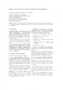
50

400 u=0.20 u=0.40 u=0.60 u=0.70

Number of tasks after clustering

Number of tasks after clustering

60

40 30 20 10 0

100

200 300 400 Number of tasks

350 300

u=0.20 u=0.40 u=0.60 u=0.70 u=0.75

250 200 150 100 50 0

500

(a) Task clustering under DM.

100

200 300 400 Number of tasks

500

(b) Task clustering under EDF.

Figure 4: Results of task clustering.

5

Experimental results

5.1

Task set generation

We chose the following model to generate random task sets: • Ui : each task utilization is computed following the classic UUnifast [6] method. We denote u the overall utilization factor of the processor. • Ti : each task period is uniformly distributed between a set of 10 periods. We observed that in industrial real-time embedded systems, the number of different tasks periods is usually limited (most often less than 10). • Ci = Ti × Ui • Di = round((Ti − Ci ) × rand(d1, d2)) + Ci with 0 ≤ d1 ≤ d2. This computation comes from [11]. We notice that d1 = d2 = 1 corresponds to implicit deadlines and d1 ≤ d2 = 1 to constrained deadlines.

5.2

Results

We have implemented the heuristic in Scala [17]. Task sets range from 50 to 500 tasks by step of 50 tasks. Maximum utilization factor is fixed at 0.70 for DM and at 0.75 for EDF. Indeed, our tests show that there is almost no schedulable task set (according to the sufficient tests used) generated above those values. We only take into account task sets that are initially schedulable in our computations. We compute average results by executing several times the heuristic on randomly generated task sets with the same parameters. We observe in Figure 4(a) that the technique is efficient under DM. Indeed, the number of tasks obtained after clustering is approximately linear in the number of tasks and the slope of the curve is rather limited. However, results under EDF test in Figure 4(b) are not as satisfying. Clustering is less efficient, especially when the utilization goes over 0.6. This difference probably comes from the fact that the clustering affects more the test under EDF than the test under DM. Indeed, the latter only alters the test on intermediary tasks when the former alters the test on all tasks with lower priority than the guest task. Finally notice that, the higher the utilization factor is, the less the tasks are clustered. Figure 5(a) and Figure 5(b) present the clustering in function of deadline bound variations with DM. For instance, [0.4 − 1.0] on the horizontal axis means that the deadline is chosen between 40% 9

nb tasks=200, u=0.60

Number of tasks after clustering

Number of tasks after clustering

50 40 30 20 10

0 [0.0-1.0] [0.2-1.0] [0.4-1.0] [0.6-1.0] [0.8-1.0] [1.0-1.0] Deadline bounds

50

nb tasks=200, u=0.60

40 30 20 10 0 [0.0-0.0] [0.0-0.2] [0.0-0.4] [0.0-0.6] [0.0-0.8] [0.0-1.0] Deadline bounds

(a) Variation of deadline lower bound.

(b) Variation of deadline upper bound.

120

nb tasks=200, u=0.60

Number of tasks after clustering

Number of tasks after clustering

Figure 5: Task clustering with DM: impact of deadline bounds.

100 80 60 40 20 0 [0.0-1.0] [0.2-1.0] [0.4-1.0] [0.6-1.0] [0.8-1.0] [1.0-1.0] Deadline bounds (a) Variation of deadline lower bound.

120

nb tasks=200, u=0.60

100 80 60 40 20 0 [0.0-0.0] [0.0-0.2] [0.0-0.4] [0.0-0.6] [0.0-0.8] [0.0-1.0] Deadline bounds (b) Variation of deadline upper bound.

Figure 6: Task clustering with EDF: impact of deadline bounds. and 100% of the period minus the execution time. We can see in Figure 5(a) that the number of clusters is minimal (equal to the number of different periods) when the deadline lower bound is about 40% of the period minus the execution time. Figure 5(b) shows that no clustering is possible before that the upper bound gets to around 60%. Above that bound, the efficiency of the clustering improves steadily (the number of clusters decreases). Figure 6(a) and Figure 6(b) present the clustering for the same deadline variations with EDF. The overall trends of the curves are similar, though the clustering is overall less efficient. These results show that the deadline bounds have the most significant impact on the clustering (even more than the number of tasks for DM). Both with DM and EDF, the clustering is the most efficient with deadlines in the interval [0.5,1]. Indeed, the closer deadlines are to the period, the more margin is left for the clustering. The clustering is even maximal in that interval because we get as many tasks as the number of different periods, both for DM and EDF. Notice that according to further experiments, this remains true for a higher number of distinct periods.

10

6

Conclusion and future work

We proposed a heuristic to automatically reduce a large set of independent tasks to a smaller set, while preserving the schedulability of the task set. The current assumption that tasks are independent is quite restrictive and will be lifted in future work. The present work is meant to lay the foundations of automated task clustering, which, as far as we know, has not been studied formally before. Experimental results point out that under some ranges of deadline bounds, the clusterings are maximal (i.e. the number of tasks equals the number of periods). Now, as these ranges are actually realistic, it would be interesting to try to formally proove that we can always reach maximal clusterings for this bounds. Such a property would allow to directly gather all the tasks with the same periods without using any complex clustering algorithm.

References [1] A. Ahmadinia, C. Bobda, and J. Teich. Temporal task clustering for online placement on reconfigurable hardware. In Field-Programmable Technology (FPT), 2003. Proceedings. 2003 IEEE International Conference on, pages 359 – 362, December 2003. [2] J. Arndt. Matters Computational: Ideas, Algorithms, Source Code. Springer, 2010. [3] N. C. Audsley, A. Burns, M. F. Richardson, and A. J. Wellings. Deadline monotonic scheduling. Citeseer, 1990. [4] AUTOSAR. RTE Standard Specifications. [5] Sanjoy K. Baruah, Rodney R. Howell, and Rosier. Feasibility problems for recurring tasks on one processor, 1993. [6] E. Bini and G.C. Buttazzo. Biasing effects in schedulability measures. In 16th Euromicro Conference on Real-Time Systems, 2004. ECRTS 2004. Proceedings, pages 196 – 203, July 2004. [7] Fr´ed´eric Boniol, Pierre-Emmanuel Hladik, Claire Pagetti, Fr´ed´eric Aspro, and Victor J´egu. A framework for distributing real-time functions. In Proceedings of the 6th international conference on Formal Modeling and Analysis of Timed Systems, FORMATS ’08, pages 155–169. SpringerVerlag, 2008. [8] Adrian Curic. Implementing Lustre Programs on Distributed Platforms with Real-time Constrains. PhD thesis, University Joseph Fourier, Grenoble, 2005. [9] U.C. Devi. An improved schedulability test for uniprocessor periodic task systems. In Real-Time Systems, 2003. Proceedings. 15th Euromicro Conference on, pages 23 – 30, july 2003. [10] Julien Forget. A Synchronous Language for Critical Embedded Systems with Multiple Real-Time Constraints. PhD thesis, Universit´e de Toulouse, 2009. [11] Joel Goossens and Christophe Macq. Limitation of the hyper-period in real-time periodic task set generation. In In Proceedings of the RTS Embedded System (RTS01, page 133147, 2001. [12] Li Guodong, Chen Daoxu, Wang Daming, and Zhang Defu. Task clustering and scheduling to multiprocessors with duplication. In Parallel and Distributed Processing Symposium, 2003. Proceedings. International, page 8 pp., April 2003. [13] Joseph Y.-T. Leung and M. L. Merrill. A note on preemptive scheduling of periodic, real-time tasks. Inf. Process. Lett., pages 115–118, 1980. [14] Joseph Y-T Leung and Jennifer Whitehead. On the complexity of fixed-priority scheduling of periodic, real-time tasks. Performance evaluation, 2(4):237–250, 1982.

11

[15] Giuseppe Lipari and Enrico Bini. A methodology for designing hierarchical scheduling systems. Journal of Embedded Computing, 1(2):257–269, 2005. [16] Cheng. L. Liu and James. W. Layland. Scheduling algorithms for multiprogramming in a hardreal-time environment. Journal of the ACM, 20(1):46–61, January 1973. [17] M. Odersky, L. Spoon, and B. Venners. Programming in Scala, 2/e. Artima Series. Artima Press, 2010. [18] Claire Pagetti, Julien Forget, Fr´ed´eric Boniol, Mikel Cordovilla, and David Lesens. Multitask implementation of multi-periodic synchronous programs. Discrete Event Dynamic Systems, 21(3):307–338, 2011. [19] M.A. Palis, Jing-Chiou Liou, and D.S.L. Wei. Task clustering and scheduling for distributed memory parallel architectures. Parallel and Distributed Systems, IEEE Transactions on, 7(1):46 –55, January 1996. [20] Krithi Ramamritham. Allocation and scheduling of precedence-related periodic tasks. IEEE Trans. Parallel Distrib. Syst., 6(4):412420, April 1995. [21] Gian-Carlo Rota. The number of partitions of a set. The American Mathematical Monthly, 71(5):498–504, 1964. [22] Stuart J. Russell and Peter Norvig. Artificial Intelligence: A Modern Approach, pages 94–95. Prentice Hall, 2 edition, 2003. [23] O. Scheickl and M. Rudorfer. Automotive real time development using a timing-augmented AUTOSAR specification. Proceedings of ERTS2008, 4, 2008. [24] S. Schliecker, J. Rox, M. Negrean, K. Richter, M. Jersak, and R. Ernst. System level performance analysis for real-time automotive multicore and network architectures. IEEE Transactions on Computer-Aided Design of Integrated Circuits and Systems, 28(7):979 –992, July 2009. [25] N. J. A. Sloane. The http://oeis.org/A000292A000292.

On-Line

Encyclopedia

of

Integer

Sequences.

[26] Ming Zhang and Zonghua Gu. Optimization issues in mapping AUTOSAR components to distributed multithreaded implementations. In 2011 22nd IEEE International Symposium on Rapid System Prototyping (RSP), pages 23 –29, May 2011.

12