automated state–dependent importance sampling ... - Semantic Scholar

Applied Probability Trust (16 September 2013)

AUTOMATED STATE–DEPENDENT IMPORTANCE SAMPLING FOR MARKOV JUMP PROCESSES VIA SAMPLING FROM THE ZERO–VARIANCE DISTRIBUTION ADAM W. GRACE,∗ The University of Queensland DIRK P. KROESE,∗ The University of Queensland

WERNER SANDMANN,∗∗ University of Derby

Abstract Many complex systems can be modeled via Markov jump processes. Applications include chemical reactions, population dynamics, and telecommunication networks. Rare-event estimation for such models can be difficult and is often computationally expensive, because typically many (or very long) paths of the Markov jump process need to be simulated in order to observe the rare event.

We present a state-

dependent importance sampling approach to this problem that is adaptive and uses Markov chain Monte Carlo to sample from the zero-variance importance sampling distribution. The method is applicable to a wide range of Markov jump processes and achieves high accuracy, while requiring only a small sample to obtain the importance parameters. We demonstrate its efficiency through benchmark examples in queueing theory and stochastic chemical kinetics. Keywords: Importance sampling, adaptive, automated, improved crossentropy, state-dependent, zero-variance distribution, Markov jump process, continuous-time Markov chain, stochastic chemical kinetics, queueing system. 2010 Mathematics Subject Classification: Primary 60J28 Secondary 62M05

∗

Postal address: School of Mathematics and Physics, The University of Queensland, Brisbane 4072, Australia Postal address: School of Computing and Mathematics, University of Derby, Derby DE22 1GB, UK

∗∗

1

2

A. W. Grace ET AL.

1. Introduction Many real-world random systems can be described mathematically via Markov jump processes. Typical examples can be found in stochastic chemical kinetics [9, 14, 18, 21], population dynamics [5, 20], and queueing networks [1, 12, 26]. Rare-event probability estimation by direct simulation of the model (crude Monte Carlo) is computationally difficult, because typically a huge simulation effort is required to observe only a few rare events. A more sophisticated approach is to use importance sampling, where the system is simulated under a change of measure, see e.g. [2, 10, 15]. However, the efficiency of this technique depends crucially on (a) the appropriate choice of a parameterized family of importance sampling distributions, and (b) the judicious selection of an appropriate member within that family; that is, the correct choice of an importance sampling parameter. Adaptive techniques such as the cross-entropy method [23] are useful for estimating good importance sampling parameters, but in high-dimensional settings it may take a large simulation effort [4]. The matter is further complicated by the fact that good importance sampling distributions often need to be state-dependent, where the importance sampling parameter depends on the state of the process. In this paper we propose a new method for obtaining state-dependent importance sampling parameters that exploits the dynamic nature of Markov jump processes. We demonstrate how to obtain, for a broad class of Markov jump processes, a state-dependent change of measure that gives improved accuracy compared to standard importance sampling approaches and recent state-dependent methods [6, 7, 22, 8, 3]. The method requires a considerably smaller sample run than current techniques to obtain suitable importance sampling parameters, due to the fact that the pilot samples are generated directly from the zero-variance distribution, using the hit-and-run Markov chain Monte Carlo sampler [24, 25]. The effectiveness of the approach is demonstrated via a range of examples in stochastic chemical kinetics and queueing theory, showing a marked improvement over existing benchmark models. The rest of the paper is organized as follows. In Section 2 we present the underlying framework for Markov jump processes used in this paper. Section 3 outlines the background for rare-event estimation and explains current approaches to estimating rare-event probabilities. We then present various improvements involving sampling from the zero-variance distribution

Automated State-Dependent Importance Sampling

3

and state-dependence importance sampling. In Section 4 we describe how to sample from the zero-variance distribution using hit-and-run Markov chain Monte Carlo sampling. In Section 5 we demonstrate the applicability and improved accuracy of the new methods via comparisons with benchmark cases in stochastic chemical kinetics and queueing theory.

2. Markov Jump Processes The class of Markov jump processes (henceforth abbreviated to MJPs) that we wish to consider has some particular structure. Firstly, the transition rates are assumed to be of the form q(x, x + yi ),

i = 1, . . . , p ,

(1)

where y1 , . . . , yp are fixed vectors. Thus, from each state x there are (at most) p different transition types that can be made by the MJP. Secondly, the transition rates depend on parameter vector u = (u1 , . . . , up ) (with ui > 0, i = 1, . . . , p), in such a way that def

qi (x; ui ) = q(x, x + yi ; ui ) = ui hi (x),

i = 1, . . . , p ,

(2)

where hi (x), i = 1, . . . , p, are non-negative functions of x. Finally, we only study the MJP in some fixed interval [0, T ]. In practice many MJPs are of this form with small or moderate p. Any path {X(t), t ∈ [0, T ]} corresponds uniquely to a sequence (t1 , r1 ), . . . , (tK , rK ), where tk is the time at which the k-th transition occurs and rk is the k-th transition type. The random variable K is the number of transitions before, and including, time T . We call J = (t1 , r1 , . . . , tK , rK ) the trajectory vector, or simply trajectory. Since the sojourn times {sk }, where sk = tk − tk−1 , are exponentially distributed, and the jump probabilities are proportional to the transition rates, we have that, for a fixed K, the probability density function (pdf) of a trajectory J is given by

f (j; u) =

K Y

k=1

 p X qi (x(tk−1 ); ui ))(tk − tk−1 ) . qrk (x(tk−1 ); urk ) exp − ( 

(3)

i=1

Simulation of the sojourn times and the transition types is straightforward via the inversetransform method [15].

4

A. W. Grace ET AL.

3. Rare-Event Probability Estimation for MJPs We wish to accurately estimate small probabilities of the form ℓ = P(J ∈ J) ,

(4)

where J is the set of all possible trajectories under which the rare event occurs. The crude Monte Carlo (CMC) estimator for ℓ is N 1 X I{J(n) ∈J} , ℓbCMC = N

(5)

n=1

iid where J(1) , . . . , J(N ) ∼ f (j; u). A measure for the accuracy of any unbiased estimator ℓb of ℓ q b is the relative error of the estimator, defined as RE = var[ℓ]/ℓ.

3.1. Importance Sampling A well-known technique to estimate rare-event probabilities more accurately than CMC is importance sampling [2, 10, 15]. The idea is to simulate the trajectories J(1) , . . . , J(N ) from a different pdf g rather than f in (3), and to estimate ℓ via the importance sampling estimator N 1 X I{J(n) ∈J} W (J(n) ) , ℓb = N

(6)

n=1

iid

where {J(n) } ∼ g and

W (J(n) ) =

f (J(n) ; u) g(J(n) )

(7)

is the likelihood ratio. Ideally one would like an importance sampling pdf g that results in the importance sampling estimator having the smallest possible variance. The best possible pdf is the zero-variance importance sampling pdf g∗ defined as the conditional pdf of J ∼ f (·; u) given J ∈ J; that is g∗ (j) =

f (j; u) I{j∈J} . ℓ

(8)

An obvious difficulty is that g∗ cannot be evaluated, since ℓ is typically not known. A useful strategy is to restrict g to the same parametric family as f and then choose from this family a member that is close, in some sense, to g∗ . Thus we consider g(j) of the form f (j; v), where v = (v1 , . . . , vp ) is the changed parameter (instead of u = (u1 , . . . , up )), and aim to find a

Automated State-Dependent Importance Sampling

5

suitable v under which to carry out the importance sampling. A possible method to use is the cross-entropy (CE) method [23], which selects a v∗ that minimizes the Kullback–Leibler (or cross-entropy) distance between g∗ and f (·; v). The standard CE method uses a multi-stage b∗ (an estimate of v∗ ) is adaptively approach, where the final importance sampling parameter v

b∗ corresponding to a sequence obtained through a sequence of parameters v[1] = u, v[2] , . . . , v

of increasingly smaller sets J[1] ⊃ J[2] ⊃ . . . ⊃ J. The optimal CE parameter v∗ is the solution to the cross-entropy optimization program [23, Section 3.3]

max Eu [W (J; u, v)I{J∈J} ln f (J; v)] ,

(9)

v

where f is given in (3) and W (J; u, v) = f (J; u)/f (J; v). Moreover, v∗ can be estimated from simulation by solving the stochastic counterpart of (9), replacing the expectation with a sample average. For the type of MJPs considered in this paper this leads to the following updating formula for the importance sampling parameters at the b-th stage of the CE procedure:

[b] vi

=

PN

(n) ; u, v[b−1] ) m(n) I {J(n) ∈J[b] } n=1 W (J i PN P (n) K (n) ; u, v[b−1] ) (n) (t(n) ))(t(n) − t(n) ) I (n) [b] n=1 W (J k=1 hi (x k−1 {J ∈J } k k−1

[b]

(n)

where vi is the i-th component of v[b] , with b = 1, 2, 3, . . ., and mi

,

(10)

is the number of type-i

iid

transitions in J(n) . Here J(1) , . . . , J(N ) ∼ f (j; v[b−1] )) are the trajectories generated at stage

b − 1. At the b-th stage of the CE procedure, J[b] is defined as the set containing all possible trajectories (not only the ones that are generated) that are “at least as rare” (according iid

to some problem-dependent criterion) as the N ̺-th rarest from the sample J(1) , . . . , J(N ) ∼

f (j; v[b−1] ). The parameter ̺ ∈ (0, 1) is fixed in advance; we typically choose ̺ = 0.1. J[1] can simply be defined as the set of all possible trajectories J. 3.2. State-Dependent Importance Sampling The family of importance sampling pdfs obtained by changing the parameters {ui } to {vi }

in (2) may not be close enough to the ideal importance sampling pdf g∗ to yield accurate

importance sampling estimates. It is natural to seek to enlarge the class of importance sampling distributions to include state-dependent changes of measure, in which the parameters {vi } depend on the state of the process. We propose to replace the transition rate of type i

6

A. W. Grace ET AL.

transitions, qi (x; ui ) in (2), with the transition rate qi (x; vi (x)) = hi (x) vi (x), where vi (x) =

βi X

vij I{x∈Bij } ,

i = 1, . . . , p ,

(11)

j=1

where the bins Bij , j = 1, . . . , βi , i = 1, . . . , p form p separate partitions of the state space E of the MJP; that is, for each i, the sets Bi1 , . . . , Biβi are disjoint and their union is E. Thus, if x ∈ Bij the transition rate from x to x + yi (see (1)) is vij hi (x). This family includes the original pdf — set βi = 1 and take Bi1 = E and vi1 = ui for i = 1, . . . , p. Because the corresponding family of importance sampling distributions includes the stateindependent one discussed in the previous section, importance sampling with the extended family can offer higher accuracy in estimation, provided the parameters {vij } are chosen appropriately. Again this can be achieved adaptively via the CE method. Similarly to (10) and (17) the parameters in the multilevel CE procedure are updated as P P (n)  N (n) ; u, v[b−1] ) n=1 I{J(n) ∈J[b] } W (J

[b]

vij = P N

(n) ; u, v[b−1] ) n=1 I{J(n) ∈J[b] } W (J

K k=1

I{rk =i} I{x(tk−1 )∈Bij }



, PK (n)  h (x(t ))(t − t )I i k−1 k k−1 {x(tk−1 )∈Bij } k=1

iid

where J(1) , . . . , J(N ) ∼ f (j; v[b−1] ). Note that we have suppressed the superscript

(n)

(12)

on rk , [b]

x, tk , and tk−1 for ease of notation. Also, the set of importance sampling parameters {vij } is

summarized as v[b] .

How to determine the partition {Bij } for each i is problem dependent. A natural approach is to partition the state space into regions within which the transition rates are roughly constant. Of course there is a trade-off between a higher number of smaller regions with nearconstant transition rate (thus leading to a more accurate change of measure) and fewer regions that possibly differ significantly but offer much less computational burden. A convenient way to partition the state space is to assign, for each type of transition i, a numerical value to the states, say φi (x) ∈ [0, 1], and to define (j−1)

Bij = {x : φi (x) ∈ (ci

(0)

where, for each i, the values 0 = ci

(j)

, ci ]} , (1)

< ci

j = 1, . . . βi , (βi )

< · · · < ci

i = 1, . . . , p,

(13)

= 1 partition up the unit interval

(0, 1]. Such an approach was taken by [22], where the function φi is defined as the probability that the MJP leaves state x via the i-th type of transition under the original measure; that

Automated State-Dependent Importance Sampling

7

is, φi (x) = qi (x; ui )/

p X

qk (x; uk ) ,

i = 1, . . . , p .

(14)

k=1

We use such a partition for all the chemistry-related examples in this paper. In general, the choice of the partition function is problem dependent and might require some experimentation to identify the regions {Bij } of interest. In the queueing Example 4, for example, we use instead φi (x) = min{xj /Ci , 1} for some constant Ci and some index j ∈ {1, . . . , d}. (j)

We next describe a simple automatic procedure for choosing the {ci } at the b-th stage

of the CE method, based on an iid sample of trajectories J(1) , . . . , J(N ) from f (j; v[b−1] ). Let (n)

xk , k = 1, . . . , K (n) , n = 1, . . . , N be the subsequent states visited by the trajectories/paths, (n)

and denote by φmin the smallest of the φi (xk ) for which the rare event at the b-th stage is i (n)

reached. Thus, we take into account only those xk (n)

xk

for which J(n) ∈ J[b] . Similarly, for such

let φmax be the maximum of the φi values. For a given βi (say βi = 10) choose i (j)

ci (0)

Recall that ci

= φmin + i (βi )

= 0 and ci

φmax − φmin i i ×j , βi

j = 1, . . . , βi − 1 .

(15)

= 1 by definition. (j)

Although (15) provides a convenient initial construction of the partitions, the {ci } (or,

∗ can be equivalently, the {Bij }) should be chosen such that the CE optimal parameters vij

accurately estimated via (12). This requires that enough transitions of type i occur when the MJP is in each set {Bij , j = 1, . . . , βi }. In particular, we require that there are at least ω type i transitions occurring in each set, where ω is specified in advance; in this paper we take ω = 20 for all examples. For partitions of the form (14) this requirement can be met (and automated) by merging (j)

(j+1)

adjacent intervals (ci , ci

(j+1)

] and (ci

(j+2)

, ci

]. The merging can be implemented in various

ways. As a numerical example, let ω = 5 and suppose (for a certain i) the interval (0, 1] is initially partitioned as (0, 0.3], (0.3, 0.4], (0.4, 0.5], (0.5, 0.6], (0.6, 0.7], (0.7, 1]. Suppose that 20 type-i transitions have taken place that have reached the (intermediate) rare event and that the counts of the numbers of times that φi (x) falls in one of the above six sets are 2, 3, 4, 2, 8, 1. Merging intervals from left to right until the combined count is more than ω, the modified partition is (0, 0.4], (0.4, 0.6], (0.6, 1], with counts 5, 6, 9.

8

A. W. Grace ET AL.

Algorithms 1 and 2 explain how the corresponding state-dependent cross-entropy method is implemented, using the method described above and as in [22]. Below, Nv is the size of the sample used to calculate the importance parameter vector v. Typically Nv is smaller than N which is used in the final simulation (6) to estimate ℓ. Algorithm 1. (Adaptive State-Dependent Cross-Entropy Method.) 1. Choose parameters ω, N , Nv , ̺, β1 , . . . , βp , and functions φi , i = 1, . . . , p. Set b = 1 and Bi1 = E, vi1 = ui for all i = 1, . . . , p. 2. Generate via Algorithm 2 an iid sample J(1) , . . . , J(Nv ) from f (j; v[b] ). 3. Let b = b + 1 and identify the elite sample as the Nv ̺ rarest of the J(1) , . . . , J(Nv ) (according to some problem-dependent criterion). If more than Nv ̺ of the generated samples fall in J, set J[b] = J; otherwise, define J[b] as the set containing all possible trajectories that are ‘at least as rare’ as the worst of the elite sample. (j)

4. Using the elite sample, determine the ci

according to (15) and further modify these to

obtain at least ω counts in each set Bij (this may change the βi ). [b]

5. Use the same elite sample to find the importance sampling parameters vij via (12). 6. If J 6= J[b] repeat Steps 2 to 5; otherwise, proceed to Step 7.

iid b∗ ), where v b∗ = v[b] . 7. Calculate ℓb via (6) using J[1] , . . . , J[N ] ∼ f (j; v

In general, the trajectory J = (t1 , r1 , . . . , tK , rK ) should be generated long enough to produce the entire path {X(t), t ∈ [0, T ]}. However, often the rare event is of the form (t1 , r1 , . . . , tM , rM ) ∈ J for some stopping time M < K (with respect to the sequence of (t1 , r1 ), (t2 , r2 ), . . .). In that case the generation of J can be stopped immediately after the rare-event occurs, say at some random stopping time τ < T . All numerical examples in this paper are of this form and the following generation algorithm is formulated accordingly. Algorithm 2. (Trajectory/Path Generation with Importance Sampling.) [b]

1. Identify J[b] and the importance sampling parameters vij . Let Nv be the sample size, and let T be the maximum time-length. Set n = 1. 2. Set t0 = 0, W (n) = 1, and k = 1; initialize X(0) = x(0).

Automated State-Dependent Importance Sampling

9

3. Generate the transition type rk and sojourn time sk using qi (x; vi (x)) = hi (x)vi (x) instead of qi (x; ui ), where vi (x) is given in (11). Set k = k + 1. 4. If tk−1 + sk > T , stop the trajectory generation and continue to Step 5. Otherwise set X(tk ) = X(tk−1 ) + yrk , tk = tk−1 + sk , and update the likelihood ratio of the n-th trajectory using

W

(n)

=W

(n)

urk exp ×



vrk (x(tk−1 )) exp



P − ( pi=1 ui hi (x(tk−1 )))sk



P − ( pi=1 vi (x(tk−1 ))hi (x(tk−1 ))sk

.

If the current J ∈ J stop the trajectory generation and continue to Step 5. Otherwise repeat from Step 3. 5. If n = Nv , stop and output J(1) , . . . , J(Nv ) and the corresponding likelihood ratios W (1) , . . . , W (Nv ) ; otherwise; set n = n + 1 and repeat from Step 2. 3.3. Improved CE The standard multilevel CE approach requires a large enough sample in each level to estimate the final importance sampling parameter vector v∗ accurately enough. Difficulties may arise when the number of parameters to be estimated is large. An alternative approach, discussed in [4] is to estimate v∗ via a single step, by (approximately) generating directly from the zero-variance pdf g∗ using, for example, Markov chain Monte Carlo methods. Specifically, b∗ of the optimal importance sampling parameter v∗ is in this case the solution the estimate v to the optimization problem

max v

where

iid J(1) , . . . , J(N ) ∼

g∗ .

N X

ln f (J(n) ; v) ,

(16)

n=1

Note that this solution is simply the maximum likelihood estimate

(MLE) of v based on the data from g∗ . Here every simulated trajectory J(n) is in J and therefore the optimal importance parameter for the MJP is estimated in a single step with a simpler version of (10): vbi∗

PN

(n) n=1 mi PK (n) (n) (t(n) ))(t(n) n=1 k=1 hi (x k k−1

=P N

(n)

− tk−1 )

,

(17)

iid

for a sample of N trajectories J(1) , . . . , J(N ) ∼ g ∗ . This parameter updating formula is more

accurate than (10). Therefore only a very small sample from g∗ is required. In Section 4 we

10

A. W. Grace ET AL.

discuss how the hit-and-run sampler can be used efficiently to sample (approximately) from g∗ . We extend the idea of state-dependent importance sampling outlined in Section 3.2 by capitalising on the improved CE formula (17). As a direct result of improved statistical inference due to sampling from g∗ , the number of bins β described in Section 3.2 can be increased. An increase in the number of bins, all with a reduced size, results in a more ‘finetuned’ change of measure that offers more accuracy in estimation. The importance sampling parameters are calculated, similarly to (12), via  PK (n)  I I {rk =i} {x(tk−1 )∈Bij } k=1 n=1 ∗ ,  vbij =P P (n) N K h (x(t ))(t − t )I i k−1 k k−1 {x(tk−1 )∈Bij } n=1 k=1 PN

iid

where J(1) , . . . , J(N ) ∼ g∗ .

(18)

Note that here there are no likelihood ratio terms and the

parameters are updated in a single step.

4. Sampling from the Zero–Variance Distribution In this section we explain how Markov chain Monte Carlo, in particular hit-and-run sampling, can be used to sample trajectories that are approximately from the zero–variance distribution. The hit-and-run sampler has been shown to be very useful in rare-event simulation (and estimation) in [11]. We present a new and powerful adaptation of hit-and-run sampling. Specifically, we apply it to static uniform vectors representing transformed dynamic MJPs. Via the inverse tranfom method a vector ξ = (ξ1 , . . . , ξV ) of iid U(0, 1) random variables can be transformed into a sequence of exponential and categorical random variables to simulate random trajectories as in (3). V is a fixed integer large enough to account for the times and types of any trajectory. Any given trajectory J can therefore be represented as J = ψ(ξ) for some function ψ. Our aim is to generate a Markov chain of trajectories ξ (0) , . . . , ξ (Nv ) that, when transformed, approximately give a random sample J(0) , . . . , J(Nv ) from g ∗ from (8). Section 4.2 explains how to obtain the initial trajectory J(0) .

Automated State-Dependent Importance Sampling

11

4.1. Zero–Variance Sampling Via Hit-and-Run Sampler This section explains how the hit-and-run sampler [24, 25] is used to construct a Markov process that converges in distribution to the uniform distribution on the set {ξ ∈ [0, 1]V : ψ(ξ) = j ∈ J}.

(19)

The hit-and-run method was chosen, instead of, for example, the Metropolis–Hastings or Gibbs samplers, because of its fast mixing properties [17] and ease of implementation. In this paper we use a modification of the hit-and-run sampler in [15, Page 242, Example 6.5]. The idea is that sampling uniformly on a region R in the hypercube is equivalent to first sampling from an n-dimensional standard normal distribution in a region Φ(R) ⊂ Rn , where Φ is the

n-dimensional normal cdf, and then applying the inverse map Φ−1 . The sampling in Rn can be done via ordinary hit-and-run. We found that this approach leads to much faster convergence to the target distribution than direct hit-and-run sampling on the hypercube. The intuitive reason is that the ordinary hit-and-run sampler will spend a lot of time in the corners of the hypercube, whereas the transformed one will search the hypercube more evenly. Algorithm 3 outlines how, starting from an initial random vector ξ (0) ∈ [0, 1]V such that ψ(ξ (0) ) = J(0) ∈ J, we can generate a Markov chain whose limiting distribution is the uniform distribution on (19). Algorithm 3. (Hit-and-Run Sampler.) 1. Obtain a ξ (0) such that ψ(ξ (0) ) = J(0) ∈ J and set n = 0. 2. Generate a random direction column vector d uniformly on the surface of the n-dimensional hypersphere. This can be done via d = √ d⊤1

d1 d1

, with d1 ∼ N(0, IV ).

3. Generate a point η (n+1) = Φ(Φ−1 (ξ (n) ) + λd) on the line segment L , via λ = −d⊤ Φ−1 (ξ (n) ) + Z,

(20)

where Z ∼ N(0, 1) and Φ and Φ−1 are the n-dimensional normal cdf and n-dimensional inverse normal cdf, respectively. 4. If ψ(η (n+1) ) = J(n+1) ∈ J set ξ (n+1) = η (n+1) . Otherwise repeat Step 3. 5. Let n = n + 1 and repeat from Step 2.

12

A. W. Grace ET AL.

Since the vectors ξ (0) , ξ (1) , ξ (2) , . . . in the Markov chain are dependent, it is necessary to apply thinning in order to obtain an approximately iid sample (of size Nv ) from the zerovariance distribution. In particular, we can keep the k-th, 2k-th, 3k-th, etc., of the generated vectors and discard the rest. There is obviously a trade-off between computational time to generate a sample and how closely the sample resembles a true random sample that is iid from g∗ . For the types of MJPs investigated in this paper we have selected k to be rather high, because in general Markov samplers in high-dimensional spaces tend to mix poorly. Therefore a total of kNv vectors corresponding to rare-events should be generated to obtain a sample of v Nv iid vectors from g∗ . After transforming, the resulting ⌊ kN k ⌋ vectors represent a random

iid

sample from the zero–variance distribution: J(k) , J(2k) , J(3k) , . . . ∼ g∗ . Note that J(0) should be discarded as it was not generated from g∗ .

4.2. Markov Sampling to Obtain Initial Rare-Event Trajectory Hit-and-run sampling is used to obtain the initial rare-event trajectory J(0) = ψ(ξ (0) ) which is then used to generate the Markov chain described in Algorithm 3. Beginning with a random uniform vector ξ ∈ U(0, 1)V , hit-and-run Markov sampling is applied such that every subsequent vector in the chain is rejected unless it is ‘as rare’ or ‘more rare’ than the current step. Algorithm 4 below describes this process. Algorithm 4. (Generate Rare-Event Trajectory.) 1. Generate ξ(0) ∼ U(0, 1)V and set n = 0. 2. Same as Step 2 in Algorithm 3. 3. Same as Step 3 in Algorithm 3. 4. Set ξ n+1 =

  η (n+1)  ξ (n)

if ψ(η (n+1) ) = J(n+1) is ‘at least as rare’ as ψ(ξ (n) ) = J(n)

(21)

otherwise .

5. Let n = n + 1 and repeat Steps 2 to 4 until ψ(ξ (n+1) ) = J(n+1) ∈ J. Remark 1. Steps 3 and 4 in Algorithm 3 involve standard acceptance-rejection sampling on a line. We denote the average “acceptance rate” by κ; that is, the expected number of samples required to generate a new point in the hit-and-run algorithm. Therefore, the total

Automated State-Dependent Importance Sampling

13

number of trajectories required to be simulated in order to obtain Nv iid trajectories from g∗ is approximately kκNv . For all the problems in this paper we have used ω = 20, k = 100 and V = 1000. All of these parameters could have been lower without significantly compromising accuracy. We have found that the computational effort required to 1) generate J(0) , 2) merging the Bij ’s, 3) calculating the importance parameters (via CE formulas), and 4) selecting the appropriate importance parameter at each step in the trajectory, is mostly negligible compared to the subsequent effort required to generate J(1) , . . . , J(Nv ) . Therefore, it is reasonable to compare the effort required for rare-event estimation in this paper by simply comparing N +Nv ×(number of iterations necessary to obtain v∗ ), for the iterative importance sampling approaches, to N +kκNv for the zero-variance approach. Note that often the final simulation is more computationally intensive than the techniques of obtaining the importance parameters. Thus, this investigation focuses primarily on the accuracy of rare-event estimation techniques. Empirical results have shown to us that our proposed approach of combining Algorithms 3 and 4 is a practical method for generating rare-events from the types of MJPs investigated in this paper. The computational effort required by our method is discussed and compared with the outlined importance sampling approaches where relevant in this paper.

5. Numerical Results In this section we demonstrate, via a range of examples, that the proposed method provides an effective approach to rare-event estimation for MJPs.

The improvement outlined in

Section 3.3 is completely adaptive and automatic. In particular, no prior knowledge of any optimal importance distribution is required. The advantages of the approach are 1), greater accuracy in estimating rare-event probabilities, 2) general applicability and 3) only a small size is required to estimate the importance sampling parameters via standard maximum likelihood. We also illustrate that Markov chain Monte Carlo can be effective, even for multi-dimensional MJPs, in sampling from the zero–variance distribution. In particular the inverse transform method combined with hit-and-run sampling is a practical way to sample vectors that are from, or extremely close to, g∗ . This has another advantage that even specific structures in trajectories from g∗ are preserved when using this method, as will be illustrated in Example 5.

14

A. W. Grace ET AL.

5.1. Stochastic Chemical Kinetics In this section we consider rare-event estimation for MJPs that represent the numbers of species in a chemical reaction. Example 1. (Chemical Reaction with Two Species.) In [22] a chemical reaction with two species of molecules is considered which can be modeled via an MJP {(X1 (t), X2 (t)), t > 0} on the positive integers, with reaction rates q((x1 , x2 ), (x1 − 1, x2 + 1)) = u1 x1 q((x1 , x2 ), (x1 + 1, x2 − 1)) = u2 x2 .

(22)

Table 1 lists the results of three importance sampling procedures for the estimation of the probability P(max06t610 X2 (t) > 30). The first method (standard CE) uses the standard state-independent CE method, where the change of measure involves the change of parameters from (u1 , u2 ) to (v1 , v2 ). The second method (state-dep. CE) implements the state-dependent multilevel Algorithm 1. In the third method (zero-variance (ZV) state-dep. CE), the singlelevel state-dependent CE procedure is used, where the importance sampling parameters are found via (18) by sampling from the zero-variance distribution. Recall that Nv is the sample size required to estimate v and β is the number of bins for each transition (reaction) type. Table 1: Numerical comparisons for P(max06t610 X2 (t) > 30) starting from X(0) = (100, 0).

standard CE

0.093

ℓb

1.42E-05

106

105

-

state-dep. CE

0.0016

1.192E-05

106

105

10

ZV state-dep CE

0.00079

1.191E-05

106

103

50

method

relative error

N

Nv

β

As can be seen in Table 1 the relative error decreases when β is increased, even when Nv , the sample size used to obtain the importance sampling parameters, is decreased. Two parameter updates were required for the first two methods but only a single update is necessary for the ZV state-dep CE method. The acceptance rate value was κ ≈ 1.2. These estimates are consistent with the true value ℓ = 1.191 × 10−5 in [22].

The numerical results below show that the proposed method(s) can deal effectively with much more elaborate systems.

Automated State-Dependent Importance Sampling

15

Example 2. (Protein Cycle Process.) As a benchmark model for stochastic chemical kinetics we consider a pheromone-induced G-protein cycle in Saccharomyces cerevisiae (see [13, 22]), which can be modeled via a seven-dimensional MJP with system state at time t represented by the vector X(t) = (X1 (t), X2 (t), X3 (t), X4 (t), X5 (t), X6 (t), X7 (t))⊤ and with transition rates q((x1 , x2 , x3 , x4 , x5 , x6 , x7 ), (x1 + 1, x2 , x3 , x4 , x5 , x6 , x7 )) = u1 q((x1 , x2 , x3 , x4 , x5 , x6 , x7 ), (x1 − 1, x2 , x3 , x4 , x5 , x6 , x7 )) = u2 x1 q((x1 , x2 , x3 , x4 , x5 , x6 , x7 ), (x1 − 1, x2 , x3 + 1, x4 , x5 , x6 , x7 )) = u3 x1 x2 q((x1 , x2 , x3 , x4 , x5 , x6 , x7 ), (x1 + 1, x2 , x3 − 1, x4 , x5 , x6 , x7 )) = u4 x3 q((x1 , x2 , x3 , x4 , x5 , x6 , x7 ), (x1 , x2 , x3 − 1, x4 − 1, x5 + 1, x6 + 1, x7 )) = u5 x3 x4 q((x1 , x2 , x3 , x4 , x5 , x6 , x7 ), (x1 , x2 , x3 , x4 , x5 − 1, x6 , x7 + 1)) = u6 x5 q((x1 , x2 , x3 , x4 , x5 , x6 , x7 ), (x1 , x2 , x3 , x4 + 1, x5 , x6 − 1, x7 − 1)) = u7 x6 x7 q((x1 , x2 , x3 , x4 , x5 , x6 , x7 ), (x1 , x2 , x3 + 1, x4 , x5 , x6 , x7 )) = u8 .

In this example there are p = 8 transition types corresponding to eight different types of chemical reactions, where u = (0.0038, 0.0004, 0.042, 0.010, 0.011, 0.100, 1050, 3.21). Suppose the rare event of interest is here: {max06t65 X6 (t) > 40}, starting from state X(0) = (50, 2, 0, 50, 0, 0, 0). We implemented the standard CE, the state-dependent multilevel CE, and the state-dependent improved CE method to calculate v and for each method used importance sampling with the same sample size N = 106 . The results are shown in Table 2. Table 2: Estimation of P(max06t65 X6 (t) > 40) starting from X(0) = (50, 2, 0, 50, 0, 0, 0).

standard CE

0.14

ℓb

2.48E-11

106

105

-

state-dep. CE

0.031

2.35E-11

106

105

10

ZV state-dep. CE

0.017

2.35E-11

106

103

50

method

relative error

N

Nv

β

The results improve those in [22] by providing a significantly lower relative error for the last method, while requiring a similar sized pilot run. For this problem the acceptance rate

16

A. W. Grace ET AL.

was κ ≈ 2.58 giving an intial sample size of approximately κkNv = 258, 000. Note that the

discrepancy in reported values of ℓb in Table 2 and [22] is due to rounding errors in the reported

transition vector u in [22].

We see that ZV state-dependent CE achieved higher accuracy than state-dependent CE (and standard CE). Increasing the number of bins β increases the accuracy of the estimate, as long as the importance sampling parameters for each bin can be calculated with sufficient accuracy. The minimum number of samples per bin ω was set at 20. The standard CE and state-dependent CE methods required four parameter updates each using Nv = 105 for each update to obtain the importance sampling parameters. Sampling from the zero-variance distribution needed a single update with only Nv = 103 . As the rareevent ℓ to be estimated becomes smaller, sampling from g∗ becomes increasingly more efficient compared with standard updating CE methods. 5.2. Tandem Jackson Queue Rare-event probability estimation problems have been studied extensively in the context of queueing systems. An important benchmark model is the tandem Jackson network. In this system customers arrive to the first queue according to a Poisson process with rate λ and are served by a single server in the order in which they arrive. If a customer arrives when the server is busy serving another customer, the arriving customer joins the end of the waiting line. Once the service is completed the customer moves on to the second queue, where the customer waits until served by the second server. The first and second servers have exponential service times with rates µ1 and µ2 , respectively. Let X1 (t) and X2 (t) be the number of customers in the first and second queue, respectively (including the customers who are being served), at time t. Then {(X1 (t), X2 (t)), t > 0} is a MJP with p = 3 transition types, with transition rates q((x1 , x2 ), (x1 + 1, x2 )) = λ q((x1 , x2 ), (x1 − 1, x2 + 2)) = µ1 I{x1 >1}

(23)

q((x1 , x2 ), (x1 , x2 − 1)) = µ2 I{x2 >1} , where I{xi >1} is the indicator that there is at least one customer in the i-th queue. This model is known to exhibit interesting rare-event behavior depending on the choice of the parameters λ, µ1 , and µ2 . A typical rare-event quantity of interest is the probability

Automated State-Dependent Importance Sampling

17

that the second queue reaches some high level y before it becomes empty. When µ1 > µ2 (the second queue is the bottleneck) a simple and effective way to estimate the rare event is to e = µ2 , use state-independent importance sampling with the following change of parameters λ µ e1 = µ1 , and µ e2 = λ. However, for the case µ1 < µ2 (the first queue is the bottleneck), a state-

independent change of measure does not work. In [16] a state-dependent change of measure is derived using the theory of Markov additive processes. Similar changes of measure are b∗ in [16, 19] is considered negligible compared outlined in [19]. The effort required to obtain v to the total simulation effort.

Example 3. (Tandem Queue (Simple).) Consider a tandem queue with transition rates λ = 1, µ1 = 4, µ2 = 2. Thus, the second queue is the bottleneck. We wish to estimate the probability ℓ that the second queue reaches 25 before it becomes empty, starting from state (1, 1). Table 3 compares the estimates and relative error from [16] (KN) with the zero-variance state-dependent CE method. For the latter we have used a function φi of the form (14) to partition the state space. Note that in this case there are only two possible values for each φi . This is because the MJP stops as soon as X2 = 0 thus making φi (x) = φi (x) =

qi λ+µ2 ,

qi λ+µ1 +µ2

or

the latter occurring when x1 = 0, where qi = λ, µ1 I{x1 >1} and µ2 I{x2 >1} for

i = 1, 2 and 3, respectively. Table 3: Estimation of the probability ℓ that the second queue reaches level 25 before becoming empty, starting from X(0) = (1, 1).

method

relative error

KN state-dep

0.0011

ZV state-dep. CE

0.0011

ℓb

4.47 × 10−8 4.48 × 10−8

N

Nv

β

106

-

-

106

104

2

We see that both methods had the same level of accuracy, showing that the automated method successfully finds the state-independent importance sampling parameters for this case. Example 4. (Tandem Queue (Difficult).) We consider the same problem as in the previous example, but now with parameter values λ = 1, µ1 = 2, µ2 = 3, which makes queue 1 the bottleneck. As mentioned before, in this case state-independent importance sampling does not work. For this problem the bins were calculated in relation to the population sizes at

18

A. W. Grace ET AL.

each queue, rather than the relative probabilities as in (14). In particular, we took φ1 (x) = min(x1 /C1 , 1), φ2 (x) = min(x1 /C2 , 1), φ3 (x) = x2 /C3 , where C1 , C2 and C3 are all 20. This is somewhat similar to the type of dependence along the state space boundaries used in general in [19]. The nature of φ1 , φ2 and φ3 used here is more suitable for this problem, and queueing problems in general. This is because the transition functions have indicator variables in relation to the distribution (population in each queue). As such, φi functions similar to (14), which was implemented in Example 3, do not utilize all of the possible statistical information to break up the state space and assign importance sampling parameters — Example 3 only had two bins for each transition! The method applied to this particular example takes into account how many customers are in each queue at every step of the Markov process. We applied zero-variance state-dependent CE and compared it with the state-dependent method in [16] (KN). The results are shown in Table 4. Table 4: Estimation of the probability ℓ that the second queue reaches level 20 before becoming empty, starting from X(0) = (1, 1).

method

relative error

KN state-dep

0.0049

ZV state-dep. CE

0.0024

ℓb

2.05 × 10−11 2.04 × 10−11

N

Nv

β

106

-

-

106

104

10

This particular choice for the φ functions (which are similar in nature to [19]) results here in a better change of measure than in [16], as is evident from the reduction in relative error for the ZV state-dep. CE method compared to the KN state-dep method used in [16]. The statedependent approach in [16] requires a numerical calculation of the importance parameters at each pre-defined bin in the state space, which is done prior to the main Monte Carlo simulation. The two other method is adaptive and automatic in its approach to calculate the state-dependent importance parameters via deterministic equations. Example 5. (Tandem Queue (Difficult 2).) As a further illustration of the methodology, consider the same model as in Example 4 where ℓ is now the probability that the second queue reaches level 20 before both queues become empty; starting from (1, 1). Table 5 shows the results for the combination-specific importance sampling, using the same φi functions as Example 4.

Automated State-Dependent Importance Sampling

19

Table 5: Estimation of the probability that the second queue reaches level 20 before both queues become empty, starting from X(0) = (1, 1).

method

relative error

ZV state-dep. CE

ℓb

1.263 × 10−9

0.0021

N

Nv

β

106

104

10

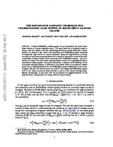
A typical rare-event trajectory for this example is shown in Figure 1. Here X1 builds up first, and while it empties into the second buffer, X2 increases “linearly” towards level 20. We have included this plot to show how sampling from the zero-variance distribution via the hit-and-run sampler can yield important information on the manner in which a rare event takes place.

Population in queues

20

X2

15

X1

10

5

0 0

2

4

6

Time

8

10

12

14

Figure 1: The first queue X1 fills up at which point the second queue X2 proceeds to overflow while X1 proceeds to empty.

Acknowledgements This work was supported by the Australian Research Council under grant number DP0985177.

References [1] S. Asmussen. Applied Probability and Queues. John Wiley & Sons, New York, 1987. [2] S. Asmussen and P. W. Glynn. Stochastic Simulation: Algorithms and Analysis. Springer-Verlag, New York, 2007.

20

A. W. Grace ET AL.

[3] J. Blanchet and H. Lam. State-dependent importance sampling for rare-event simulation: An overview and recent advances. Surveys in Operations Research and Management Science, 17:38– 59, 2012. [4] J.C.C. Chan and D.P. Kroese. Improved cross-entropy method for estimation. Statistics and Computing, DOI: 10.1007/s11222-011-9275-7, 2011. [5] J. E. Cohen. Markov population processes as models of primate social and population dynamics. Theoretical Population Biology, 3:119–134, 1972. [6] P. T. de Boer and V. F. Nicola. Adaptive state-dependent importance sampling simulation of Markovian queueing networks. European Transactions on Telecommunications, 13:303–315, 2002. [7] P. Dupuis, A. D. Sezer, and H. Wang. Dynamic importance sampling for queueing networks. Annals of Applied Probability, 17:1306–1346, 2007. [8] P. Dupuis and H. Wang. Importance sampling for jackson networks. Queueing Systems, 62:113– 157, 2009. [9] D. T. Gillespie. Exact stochastic simulation of coupled chemical reactions. The Journal of Physical Chemistry, 2:2340–2361, 1977. [10] P. W. Glynn and D. L. Iglehart. Importance sampling for stochastic simulations. Management Science, 35(11):1367–1392, 1989. [11] A. W. Grace and I. A. Wood. Approximating the tail of the Anderson–Darling distribution. Computational Statistics & Data Analysis, 56:4301–4311, 2012. [12] P. Heidelberger.

Fast simulation of rare events in queuing and reliability models.

ACM

Transactions on Modeling and Computer Simulation, 5:43–85, 1995. [13] B. J. Daigle Jr, M. K. Roh, D. T. Gillespie, and L. R. Petzold. Automated estimation of rare event probabilities in biochemical systems. The Journal of Chemical Physics, 134(4):044110, 2011. [14] N. G. Van Kampen. Stochastic processes in physics and chemistry. Elsevier, North Holland, 1992. [15] D. P. Kroese, T. Taimre, and Z. I. Botev. Handbook of Monte Carlo Methods. John Wiley & Sons, New York, 2011. [16] D.P. Kroese and V.F. Nicola. Efficient simulation of a tandem jackson network. ACM Transactions on Modeling and Computer Simulation, 12:119–141, 2002. [17] L. Lov´asz. Hit-and-run mixes fast. Mathematical Programming, 86:443–461, 1999. [18] D. A. McQuarrie. Stochastic approach to chemical kinetics. Journal of Applied Probability, 4:413–478, 1967. [19] V. F. Nicola and T. S. Zaburnenko. Efficient importance sampling heuristics for the simulation of population overflow in jackson networks. ACM Transactions on Modeling and Computer Simulation, 17:DOI – 10.1145/1225275.1225281, 2007.

Automated State-Dependent Importance Sampling

21

[20] R. Pearl. The biology of population growth. Alfred A. Knopf, New York, 1925. [21] P. K. Pollett and A. Vassallo. Diffusion approximations for some simple chemical reaction schemes. Advances in Applied Probability, 24:875–893, 1992. [22] M. K. Roh, Jr. B. J. Daigle, D. T. Gillespie, and L. R. Petzold. State-dependent doubly weighted stochastic simulation algorithm for automatic characterization of stochastic biochemical rare events. The Journal of Chemical Physics, 135(23):234108, 2011. [23] R. Y. Rubinstein and D. P. Kroese.

The Cross-Entropy Method: A Unified Approach to

Combinatorial Optimization. Springer-Verlag, New York, 2004. [24] R. L. Smith. Efficient Monte Carlo procedures for generating points uniformly distributed over bounded regions. Operations Research, 32:1296–1308, 1984. [25] R. L. Smith. The hit-and-run sampler: A globally reaching Markov chain sampler for generating arbitrary multivariate distributions. Proceedings of the 28th Conference on Winter Simulation, IEEE Computer Society, pages 260–264, 1996. [26] R. W. Wolf. Stochastic Modeling and the Theory of Queues. Prentice-Hall, Englewood Cliffs, NJ, 1989.