Automated Termination Proofs for Java Programs with Cyclic Data⋆

Automated Termination Proofs for Java Programs with Cyclic Data? Marc Brockschmidt, Richard Musiol, Carsten Otto, and J¨ urgen Giesl LuFG Informatik 2, RWTH Aachen University, Germany

Abstract. In earlier work, we developed a technique to prove termination of Java programs automatically: first, Java programs are automatically transformed to term rewrite systems (TRSs) and then, existing methods and tools are used to prove termination of the resulting TRSs. In this paper, we extend our technique in order to prove termination of algorithms on cyclic data such as cyclic lists or graphs automatically. We implemented our technique in the tool AProVE and performed extensive experiments to evaluate its practical applicability.

1

Introduction

Techniques to prove termination automatically are essential in program verification. While approaches and tools for automated termination analysis of term rewrite systems (TRSs) and of logic programs have been studied for decades, in the last years the focus has shifted toward imperative languages like C or Java. Most techniques for imperative languages prove termination by synthesizing ranking functions (e.g., [12, 26]) and localize the termination test using Ramsey’s theorem [23, 27]. Such techniques are for instance used in the tools Terminator [4, 13] and LoopFrog [22, 31] to analyze termination of C programs. To handle the heap, one can use an abstraction [14] to integers based on separation logic [24]. On the other hand, there also exist transformational approaches which automatically transform imperative programs to TRSs or to logic programs. They allow to re-use the existing techniques and tools from term rewriting or logic programming also for imperative programs. In [17], C is analyzed by a transformation to TRSs and the tools Julia [30] and COSTA [2] prove termination of Java via a transformation to constraint logic programs. To deal with the heap, they also use an abstraction to integers and represent objects by their path length. In [6–8, 25] we presented an alternative approach for termination of Java via a transformation to TRSs. Like [2, 30], we consider Java Bytecode (JBC) to avoid dealing with all language constructs of Java. This is no restriction, since Java compilers automatically translate Java to JBC. Indeed, our implementation handles the Java Bytecode produced by Oracle’s standard compiler. In contrast to other approaches, we do not treat the heap by an abstraction to integers, but by an abstraction to terms. So for any class Cl with n non-static fields, we use an n-ary function symbol Cl. For example, consider a class List with two fields value and next. Then every List object is encoded as a term List(v, n) where ?

Supported by the DFG grant GI 274/5-3

v is the value of the current element and n is the encoding of the next element. Hence, a list “[1, 2]” is encoded by the term List(1, List(2, null)). In this way, our encoding maintains much more information from the original program than a (fixed) abstraction to integers. Now the advantage is that for any algorithm, existing tools from term rewriting can automatically search for (possibly different) suitable well-founded orders comparing arbitrary forms of terms. For more information on techniques for termination analysis of term rewriting, see, e.g., [16, 20, 33]. As shown in the annual International Termination Competition,1 due to this flexibility, the implementation of our approach in the tool AProVE [19] is currently the most powerful termination prover for Java. In this paper, we extend our technique to handle algorithms whose termination depends on cyclic objects (e.g., lists like “[0, 1, 2, 1, 2, . . .]” or cyclic graphs). Up to now, transformational approaches could not deal with such programs. Similar to related approaches based on separation logic [4, 5, 10, 11, 28, 32], our technique relies on suitable predicates describing properties of the heap. Like [28], but in contrast to several previous works, our technique derives these heap predicates automatically from the input program and it works automatically for arbitrary data structures (i.e., not only for lists). We integrated this new technique in our fully automated termination analysis and made the resulting termination tool available via a web interface [1]. This tool automatically proves termination of Java programs on possibly cyclic data, i.e., the user does not have to provide loop preconditions, invariants, annotations, or any other manual pre-processing. Our technique works in two steps: first, a JBC program is transformed into a termination graph, which is a finite representation of all program runs. This graph takes all sharing effects into account. Afterwards, a TRS is generated from the graph. In a similar way, we also developed techniques to analyze termination of other languages like Haskell [21] or Prolog [29] via a translation to TRSs. Of course, one could also transform termination graphs into other formalisms than TRSs. For example, by fixing the translation from objects to integers, one could easily generate integer transition systems from the termination graph. Then the contributions of the current paper can be used as a general pre-processing approach to handle cyclic objects, which could be coupled with other termination tools. However, for methods whose termination does not rely on cyclic data, our technique is able to transform data objects into terms. For such methods, the power of existing tools for TRSs allows us to find more complex termination arguments automatically. By integrating the contributions of the current paper into our TRS-based framework, the resulting tool combines the new approach for cyclic data with the existing TRS-based approach for non-cyclic data. In Sect. 2-4, we consider three typical classes of algorithms which rely on data that could be cyclic. The first class are algorithms where the cyclicity is irrelevant for termination. So for termination, one only has to inspect a noncyclic part of the objects. For example, consider a doubly-linked list where the predecessor of the first and the successor of the last element are null. Here, a traversal only following the next field obviously terminates. To handle such 1

See http://termination-portal.org/wiki/Termination_Competition

algorithms, in Sect. 2 we recapitulate our termination graph framework and present a new improvement to detect irrelevant cyclicity automatically. The second class are algorithms that mark every visited element in a cyclic object and terminate when reaching an already marked element. In Sect. 3, we develop a technique based on SMT solving to detect such marking algorithms by analyzing the termination graph and to prove their termination automatically. The third class are algorithms that terminate because an element in a cyclic object is guaranteed to be visited a second time (i.e., the algorithms terminate when reaching a specified sentinel element). In Sect. 4, we extend termination graphs by representing definite sharing effects. Thus, we can now express that by following some field of an object, one eventually reaches another specific object. In this way, we can also prove termination of well-known algorithms like the in-place reversal for pan-handle lists [10] automatically. We implemented all our contributions in the tool AProVE. Sect. 5 shows their applicability by an evaluation on a large benchmark collection (including numerous standard Java library programs, many of which operate on cyclic data). In our experiments, we observed that the three considered classes of algorithms capture a large portion of typical programs on cyclic data. For the treatment of (general classes of) other programs, we refer to our earlier papers [6, 7, 25]. Moreover, in [8] we presented a technique that uses termination graphs to also detect nontermination. By integrating the new contributions of the current paper into our approach, our tool can now automatically prove termination for programs that contain methods operating on cyclic data as well as other methods operating on non-cyclic data. For the proofs of the theorems as well as all formal definitions needed for the construction of termination graphs, we refer to [9].

2

Handling Irrelevant Cycles

We restrict ourselves to programs without method calls, arrays, exception handlers, static fields, floating point numbers, class initializers, reflection, and multithreading to ease the presentation. However, our implementation supports these features, except reflection and multithreading. For further details, see [6–8]. class L1 { L1 p , n ; static int length ( L1 x ) { int r = 1; while ( null != ( x = x . n )) r ++; return r ; }} Fig. 1. Java Program

00: 01: 02: 03: 04: 07: 08: 09:

iconst_1 istore_1 aconst_null aload_0 getfield n dup astore_0 if_acmpeq 18

# load 1 # store to r # load null # load x # get n from x # duplicate n # store to x # jump if # x . n == null # increment r

In Fig. 1, L1 is a class for (doubly-linked) lists where n and p point to the next and previous element. For brevity, we omitted a field for the value of elements. The

12: 15: 18: 19:

iinc 1 , 1 goto 02 iload_1 # load r ireturn # return r Fig. 2. JBC for length

method length initializes a variable r for the result and traverses the list until x is null. Fig. 2 shows the corresponding JBC obtained by the Java compiler. After introducing program states in Sect. 2.1, we explain how termination graphs are generated in Sect. 2.2. Sect. 2.3 shows the transformation from termination graphs to TRSs. While this two-step transformation was already presented in our earlier papers, here we extend it by an improved handling of cyclic objects in order to prove termination of algorithms like length automatically. 2.1

Abstract States in Termination Graphs

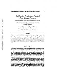
We generate a graph of abstract states from States = PPos × LocVar × OpStack × Heap × Annotations, where PPos Fig. 3. State A is the set of all program positions. Fig. 3 depicts the initial state for the method length. The first three components of a state are in the first line, separated by “|”. The first component is the program position, indicated by the index of the next instruction. The second component represents the local variables as a list of references, i.e., LocVar = Refs∗ .2 To ease readability, in examples we denote local variables by names instead of numbers. So “x : o1 ” indicates that the 0-th local variable x has the value o1 . The third component is the operand stack OpStack = Refs∗ for temporary results of JBC instructions. The empty stack is denoted by ε and “o1 , o2 ” is a stack with top element o1 . Below the first line, information about the heap is given by a function from Heap = Refs → Ints ∪ Unknown ∪ Instances ∪ {null} and by a set of annotations specifying sharing effects in parts of the heap that are not explicitly represented. For integers, we abstract from the different types of bounded integers in Java and consider unbounded integers instead, i.e., we cannot handle problems related to overflows. We represent unknown integers by intervals, i.e., Ints = {{x ∈ Z | a ≤ x ≤ b} | a ∈ Z ∪ {−∞}, b ∈ Z ∪ {∞}, a ≤ b}. For readability, we abbreviate intervals such as (−∞, ∞) by Z and [1, ∞) by [> 0]. Let Classnames contain all classes and interfaces in the program. The values Unknown = Classnames ×{?} denote that a reference points to an unknown object or to null. Thus, “o1 : L1(?)” means that at address o1 , we have an instance of L1 (or of its subclasses) with unknown field values or that o1 is null. To represent actual objects, we use Instances = Classnames ×(FieldIDs → Refs), where FieldIDs is the set of all field identifiers. To prevent ambiguities, in general the FieldIDs also contain the respective class names. Thus, “o2: L1(p = o3 , n = o4 )” means that at address o2 , we have some object of type L1 whose field p contains the reference o3 and whose field n contains o4 . In our representation, if a state contains the references o1 and o2 , then the objects reachable from o1 resp. o2 are disjoint3 and tree-shaped (and thus acyclic), unless explicitly stated otherwise. This is orthogonal to the default assumptions 00 | x : o1 | ε o1: L1(?) o1 {p,n}

2

3

To avoid a special treatment of integers (which are primitive values in JBC), we also represent them using references to the heap. An exception are references to null or Ints, since in JBC, integers are primitive values where one cannot have any side effects. So if h is the heap of a state and h(o1 ) = h(o2 ) ∈ Ints or h(o1 ) = h(o2 ) = null, then one can always assume o1 = o2 .

in separation logic, where sharing is allowed unless stated otherwise, cf. e.g. [32]. In our states, one can either express sharing directly (e.g., “o1 : L1(p = o2 , n = o1 )” implies that o1 reaches o2 and is cyclic) or use annotations to indicate (possible) sharing in parts of the heap that are not explicitly represented. The first kind of annotation is the equality annotation o =? o0 , meaning that o and o0 could be the same. We only use this annotation if h(o) ∈ Unknown or h(o0 ) ∈ Unknown, where h is the heap of the state. The second annotation is the joinability annotation o %$ o0 , meaning that o and o0 possibly have a common f successor. To make this precise, let o1 → o2 denote that the object at o1 has a field f ∈ FieldIDs with o2 as its value (i.e., h(o1 ) = (Cl, e) ∈ Instances π and e(f) = o2 ). For any π = f1 . . . fn ∈ FieldIDs∗ , o1 → on+1 denotes that f

f

fn−1

f

ε

there exist o2 , . . . , on with o1 →1 o2 →2 . . . → on →n on+1 . Moreover, o1 → o01 iff o1 = o01 . Then o %$ o0 means that there could be some o00 and some π and τ π τ such that o → o00 ← o0 , where π 6= ε or τ 6= ε. In our earlier papers [6, 25] we had another annotation to denote references that may point to non-tree-shaped objects. In the translation to terms later on, all these objects were replaced by fresh variables. But in this way, one cannot prove termination of length. To maintain more information about possibly nontree-shaped objects, we now introduce two new shape annotations o♦ and o FI instead. The non-tree annotation o♦ means that o might be not tree-shaped. π π More precisely, there could be a reference o0 with o →1 o0 and o →2 o0 where π1 is no prefix of π2 and π2 is no prefix of π1 . However, these two paths from o to o0 may not traverse any cycles (i.e., there are no prefixes τ1 , τ2 of π1 or of π2 where τ1 τ2 τ1 6= τ2 , but o → o00 and o → o00 for some o00 ). The cyclicity annotation o FI means that there could be cycles including o or reachable from o. However, any cycle must use at least the fields in FI ⊆ FieldIDs. In other words, if π τ o → o0 → o0 for some τ 6= ε, then τ must contain all fields from FI . We often write instead of ∅ . Thus in Fig. 3, o1 {p,n} means that there may be cycles reachable from o1 and that any such cycle contains at least one n and one p field. 2.2

Constructing the Termination Graph

Our goal is to prove termination of length for all doubly-linked lists without “real” cycles (i.e., there is no cycle traversing only n or only p fields). Hence, A is the initial state when calling the method with such an input list.4 From A, the termination graph in Fig. 4 is constructed by symbolic evaluation. First, iconst 1 loads the constant 1 on the operand stack. This leads to a new state connected to A by an evaluation edge (we omitted this state from Fig. 4 for reasons of space). Then istore 1 stores the constant 1 from the top of the operand stack in the first local variable r. In this way, we obtain state B (in Fig. 4 we use dotted edges to indicate several steps). Formally, the constant 1 is represented by some reference i ∈ Refs that is mapped to [1, 1] ∈ Ints by the heap. However, we shortened this for the presentation and just wrote r : 1. 4

The state A is obtained automatically when generating the termination graph for a program where length is called with an arbitrary such input list, cf. Sect. 5.

00 | x : o1 | ε o1: L1(?) o1 {p,n}

A

02 | x : o1 , r : 1 | ε o1: L1(?) o1 {p,n}

B

04 | x : o1 , r : 1 | o1 , null o1: L1(?) o1 {p,n}

04 | x : o2 , r : 1 | o2 , null o2: L1(p = o3 , n = o4 ) o3: L1(?) o4: L1(?) o2%$o3 o2%$o4 o3%$o4 o2 , o3 , o4 {p,n}

I0 02 | x : o05 , r : i2 | ε 09 | x : o04 , r : i1 | o04 , null o05: L1(p = o06 , n = o07 ) o04: L1(?) o04 {p,n} o06: L1(?) o07: L1(?) i2: [> 1] i2 = i1 + 1 o05 %$o06 o05 %$o07 o06 %$o07 o05 , o06 , o07 {p,n} 04 | x : o01 , r : i1 | o01 , null o01: L1(?) o01 {p,n} i1: [>0] B0 C

E

02 | x : o01 , r : i1 | ε o01: L1(?) o01 {p,n} i1: [>0] 04 | x : null, r : 1 | null, null

D

09 | x : null, r : 1 | null, null

G

09 | x : o4 , r : 1 | o4 , null o4: L1(?) o4 {p,n}

F

02 | x : o5 , r : 2 | ε o5: L1(p = o6 , n = o7 ) o6: L1(?) o7: L1(?) o5%$o6 o5%$o7 o6%$o7 o5 , o6 , o7 {p,n} 09 | x : o5 , r : 1 | o5 , null o5: L1(p = o6 , n = o7 ) o6: L1(?) o7: L1(?) o5%$o6 o5%$o7 o6%$o7 o5 , o6 , o7 {p,n}

F0

C0

I

H

Fig. 4. Termination Graph for length

In B, we load null and the value of x (i.e., o1 ) on the operand stack, resulting in C. In C, the result of getfield depends on the value of o1 . Hence, we perform a case analysis (a so-called instance refinement) to distinguish between the possible types of o1 (and the case where o1 is null). So we obtain D where o1 is null, and E where o1 points to an actual object of type L1. To get single static assignments, we rename o1 to o2 in E and create fresh references o3 and o4 for its fields p and n. We connect D and E by dashed refinement edges to C. In E, our annotations have to be updated. If o1 can reach a cycle, then this could also hold for its successors. Thus, we copy {p,n} to the newly-created successors o3 and o4 . Moreover, if o2 (o1 under its new name) can reach itself, then its successors might also reach o2 and they might also reach each other. Thus, we create %$ annotations indicating that each of these references may share with any of the others. We do not have to create any equality annotations. The annotation o2 =? o3 (and o2 =? o4 ) is not needed because if the two were equal, they would form a cycle involving only one field, which contradicts {p,n} . Furthermore, we do not need o3 =? o4 , as o1 was not marked with ♦. D ends the program (by an exception), indicated by an empty box. In E, getfield n replaces o2 on the operand stack by the value o4 of its field n, dup duplicates the entry o4 on the stack, and astore 0 stores one of these entries in x, resulting in F . We removed o2 and o3 which are no longer used in local variables or the operand stack. To evaluate if acmpeq in F , we branch depending on the equality of the two top references on the stack. So we need an instance refinement and create G where o4 is null, and H where o4 refers to an actual object. The annotations in H are constructed from F just as E was constructed from C. G results in a program end. In H, r’s value is incremented to 2 and we jump back to instruction 02, resulting in I. We could continue symbolic evaluation, but this would not yield a finite termination graph. Whenever two states like B and I are at the same program position, we use generalization (or widening [14]) to find a common representative B 0 of both B and I. By suitable heuristics,

our automation ensures that one always reaches a finite termination graph after finitely many generalization steps [8]. The values for references in B 0 include all values that were possible in B or I. Since r had the value 1 in B and 2 in I, this is generalized to the interval [> 0] in B 0 . Similarly, since x was Unknown in B but a non-null list in I, this is generalized to an Unknown value in B 0 . We draw instance edges (depicted by thick arrows) from B and I to B 0 , indicating that all concrete (i.e., non-abstract) program states represented by B or I are also represented by B 0 . So B and I are instances of B 0 (written B v B 0 , I v B 0 ) and any evaluation starting in B or I could start in B 0 as well. From B 0 on, symbolic evaluation yields analogous states as when starting in B. The only difference is that now, r’s value is an unknown positive integer. Thus, we reach I 0 , where r’s value i2 is the incremented value of i1 and the edge from F 0 to I 0 is labeled with “i2 = i1 + 1” to indicate this relation. Such labels are used in Sect. 2.3 when generating TRSs from termination graphs. The state I 0 is similar to I, and it is again represented by B 0 . Thus, we can draw an instance edge from I 0 to B 0 to “close” the graph, leaving only program ends as leaves. A sequence of concrete states c1 , c2 , . . . is a computation path if ci+1 is obtained from ci by standard JBC evaluation. A computation sequence is represented by a termination graph if there is a path s11 , . . . , sk11 , s12 , . . . , sk22 , . . . of states in the termination graph such that ci v s1i , . . . , ci v ski i for all i and such that all labels on the edges of the path (e.g., “i2 = i1 + 1”) are satisfied by the corresponding values in the concrete states. Thm. 1 shows that if a concrete state c1 is an instance of some state s1 in the termination graph, then every computation path starting in c1 is represented by the termination graph. Thus, every infinite computation path starting in c1 corresponds to a cycle in the termination graph. Theorem 1 (Soundness of Termination Graphs). Let G be a termination graph, s1 some state in G, and c1 some concrete state with c1 v s1 . Then any computation sequence c1 , c2 , . . . is represented by G. 2.3

Proving Termination via Term Rewriting

From the termination graph, one can generate a TRS with built-in integers [18] that only terminates if the original program terminates. To this end, in [25] we showed how to encode each state of a termination graph as a term and each edge as a rewrite rule. We now extend this encoding to the new annotations ♦ and in such a way that one can prove termination of algorithms like length. To encode states, we convert the values of local variables and operand stack entries to terms. References with unknown value are converted to variables of the same name. So the reference i1 in state B 0 is converted to the variable i1 . The null reference is converted to the constant null and for objects, we use the name of their class as a function symbol. The arguments of that function correspond to the fields of the class. So a list x of type L1 where x.p and x.n are null would be converted to the term L1(null, null) and o2 from state E would be converted to the term L1(o3 , o4 ) if it were not possibly cyclic. In [25], we had to exclude objects that were not tree-shaped from this translation. Instead, accesses to such objects always yielded a fresh, unknown variable.

To handle objects annotated with ♦, we now use a simple unrolling when transforming them to terms. Whenever a reference is changed in the termination graph, then all its occurrences in the unrolled term are changed simultaneously in the corresponding TRS. To handle the annotation FI , now we only encode a subset of the fields of each class when transforming objects to terms. This subset is chosen such that at least one field of FI is disregarded in the term encoding.5 Hence, when only regarding the encoded fields, the data objects are acyclic and can be represented as terms. To determine which fields to drop from the encoding, we use a heuristic which tries to disregard fields without read access. In our example, all cyclicity annotations have the form {p,n} and p is never read. Hence, we only consider the field n when encoding L1-objects to terms. Thus, o2 from state E would be encoded as L1(o4 ). Now any read access to p would have to be encoded as returning a fresh variable. For every state we use a function with one argument for each local variable and each entry of the operand stack. So E is converted to fE (L1(o4 ), 1, L1(o4 ), null). To encode the edges of the termination graph as rules, we consider the different kinds of edges. For a chain of evaluation edges, we obtain a rule whose left-hand side is the term resulting from the first state and whose right-hand side results from the last state of the chain. So the edges from E to F result in fE (L1(o4 ), 1, L1(o4 ), null) → fF (o4 , 1, o4 , null). In term rewriting [3], a rule ` → r can be applied to a term t if there is a substitution σ with `σ = t0 for some subterm t0 of t. The application of the rule results in a variant of t where t0 is replaced by rσ. For example, consider a concrete state where x is a list of length 2 and the program counter is 04. This state would be an instance of the abstract state E and it would be encoded by the term fE (L1(L1(null)), 1, L1(L1(null)), null). Now applying the rewrite rule above yields fF (L1(null), 1, L1(null), null). In this rule, we can see the main termination argument: Between E and F , one list element is “removed” and the list has finite length (when only regarding the n field). A similar rule is created for the evaluations that lead to state F 0 , where all occurrences of 1 are replaced by i1 . In our old approach [25], the edges from E to F would result in fE (L1(o4 ), 1, L1(o4 ), null) → fF (o04 , 1, o04 , null). Its right-hand side uses the fresh variable o04 instead of o4 , since this was the only way to represent cyclic objects in [25]. Since o04 could be instantiated by any term during rewriting, this TRS is not terminating. For refinement edges, we use the term for the target state on both sides of the resulting rule. However, on the left-hand side, we label the outermost function symbol with the source state. So for the edge from F to H, we have the term for H on both sides of the rule, but on the left-hand side we replace fH by fF : fF (L1(o7 ), 1, L1(o7 ), null) → fH (L1(o7 ), 1, L1(o7 ), null) For instance edges, we use the term for the source state on both sides of the resulting rule. However, on the right-hand side, we label the outermost function with the target state instead. So for the edge from I to B 0 , we have the term for 5

Of course, if FI = ∅, then we still handle cyclic objects as before and represent any access to them by a fresh variable.

I on both sides of the rule, but on the right-hand side we replace fI by fB 0 : fI (L1(o7 ), 2) → fB 0 (L1(o7 ), 2) For termination, it suffices to convert just the (non-trivial) SCCs of the termination graph to TRSs. If we do this for the only SCC B 0 , . . . , I 0 , . . . , B 0 of our graph, and then “merge” rewrite rules that can only be applied after each other [25], then we obtain one rule encoding the only possible way through the loop: fB 0 (L1(L1(o7 )), i1 ) → fB 0 (L1(o7 ), i1 + 1) Here, we used the information on the edges from F 0 to I 0 to replace i2 by i1 +1. Termination of this rule is easily shown automatically by termination provers like AProVE, although the original Java program worked on cyclic objects. However, our approach automatically detects that the objects are not cyclic anymore if one uses a suitable projection that only regards certain fields of the objects. Theorem 2 (Proving Termination of Java by TRSs). If the TRSs resulting from the SCCs of a termination graph G are terminating, then G does not represent any infinite computation sequence. So by Thm. 1, the original JBC program is terminating for all concrete states c where c v s for some state s in G.

3

Handling Marking Algorithms on Cyclic Data

public class L2 { int v ; L2 n ; static void visit ( L2 x ){ int e = x . v ; while ( x . v == e ) { x . v = e + 1; x = x . n ; }}} Fig. 5. Java Program

00: 01: 04: 05: 06: 09: 10: 13: 14: 15: 16: 17: 20: 21: 24: 25: 28:

aload_0 # load x getfield v # get v from x istore_1 # store to e aload_0 # load x getfield v # get v from x iload_1 # load e if_icmpne 28 # jump if x . v != e aload_0 # load x iload_1 # load e iconst_1 # load 1 iadd # add e and 1 putfield v # store to x . v aload_0 # load x getfield n # get n from x astore_0 # store to x goto 5 return Fig. 6. JBC for visit

We now regard lists with a “next” field n where every element has an integer value v. The method visit stores the value of the first list element. Then it iterates over the list elements as long as they have the same value and “marks” them by modifying their value. If all list elements had the same value initially, then the iteration either ends with a NullPointerException (if the list is non-cyclic) or because some element is visited for the second time (this is detected by its modified “marked” value).6 We illustrate the termination graph of visit in Sect. 3.1 and extend our approach in order to prove termination of such marking algorithms in Sect. 3.2. 6

While termination of visit can also be shown by the technique of Sect. 4 which detects whether an element is visited twice, the technique of Sect. 4 fails for analogous marking algorithms on graphs which are easy to handle by the approach of Sect. 3, cf. Sect. 5. So the techniques of Sect. 3 and 4 do not subsume each other.

05 | x : o1 ,e : i1 | ε o1: L2(?) i1: Z

A

06 | x : null,e : i1 | null

o1

06 | x : o1 ,e : i1 | o1 o1: L2(?) i1: Z o1

B

06 | x : o2 ,e : i1 | o2 D o2: L2(v = i2 , n = o3 ) o3 : L2(?) i1 : Z i2 : Z o2 ,o3 o2%$o3 o2=?o3 05 | x : o3 ,e : i1 | ε o3: L2(?) i1: Z o3

06 | x : o2 ,e : i1 | o2 o2: L2(v = i2 , n = o2 ) i1: Z i2: Z 06 | x : o2 ,e : i1 | o2 o2: L2(v = i2 , n = o3 ) o3 : L2(?) i1 : Z i2 : Z o2 ,o3 o2%$o3

J i3 = i1 +1 10 | x : o2 ,e : i1 | i1 , i1 o2: L2(v = i1 , n = o3 ) o3: L2(?) i1: Z o2 ,o3 o2%$o3

C i1 = i2 05 | x : o2 ,e : i1 | ε i4 = i1 +1 o2: L2(v = i4 , n = o2 ) F

10 | x : o2 ,e : i1 | i1 , i2 o2: L2(v = i2 , n = o2 ) i1 : Z i2 : Z

i1 6= i2

K L

10 | x : o2 ,e : i1 | i1 , i2 o2: L2(v = i2 , n = o3 ) o2%$o3 G o3: L2(?) i1: Z i2: Z o2 ,o3

E

i1 = I

i3 : Z

i2 i1 6= i2 10 | x : o2 ,e : i1 | i1 , i2 o2 : L2(v = i2 , n = o3 ) o2%$o3 H o3: L2(?) i1: Z i2: Z o2 ,o3

Fig. 7. Termination Graph for visit

3.1

Constructing the Termination Graph

When calling visit for an arbitrary (possibly cyclic) list, one reaches state A in Fig. 7 after one loop iteration by symbolic evaluation and generalization. Now aload 0 loads the value o1 of x on the operand stack, yielding state B. To evaluate getfield v, we perform an instance refinement and create a successor C where o1 is null and a successor D where o1 is an actual instance of L2. As in Fig. 4, we copy the cyclicity annotation to o3 and allow o2 and o3 to join. Furthermore, we add o2 =? o3 , since o2 could be a cyclic one-element list. In C, we end with a NullPointerException. Before accessing o2 ’s fields, we have to resolve all possible equalities. We obtain E and F by an equality refinement, corresponding to the cases o2 6= o3 and o2 = o3 . F needs no annotations anymore, as all reachable objects are completely represented in the state. In E we evaluate getfield, retrieving the value i2 of the field v. Then we load e’s value i1 on the operand stack, which yields G. To evaluate if icmpne, we branch depending on the inequality of the top stack entries i1 and i2 , resulting in H and I. We label the refinement edges with the respective integer relations. In I, we add 1 to i1 , creating i3 , which is written into the field v of o2 . Then, the field n of o2 is retrieved, and the obtained reference o3 is written into x, leading to J. As J is a renaming of A, we draw an instance edge from J to A. The states following F are analogous, i.e., when reaching if icmpne, we create successors depending on whether i1 = i2 . In that case, we reach K, where we have written the new value i4 = i1 + 1 into the field v of o2 . Since K is also an instance of A, this concludes the construction of the termination graph. 3.2

Proving Termination of Marking Algorithms

To prove termination of algorithms like visit, we try to find a suitable marking property M ⊆ Refs × States. For every state s with heap h, we have (o, s) ∈ M if o is reachable7 in s and if h(o) is an object satisfying a certain property. We add 7

Here, a reference o is reachable in a state s if s has a local variable or an operand π stack entry o0 such that o0 → o for some π ∈ FieldIDs∗ .

a local variable named cM to each state which counts the number of references in M . More precisely, for each concrete state s with “cM : i” (i.e., the value of the new variable is the reference i), h(i) ∈ Ints is the singleton set containing the number of references o with (o, s) ∈ M . For any abstract state s with “cM : i” that represents some concrete state s0 (i.e., s0 v s), the interval h(i) must contain an upper bound for the number of references o with (o, s0 ) ∈ M . In our example, we consider the property L2.v = i1 , i.e., cM counts the references to L2-objects whose field v has value i1 . As the loop in visit only continues if there is such an object, we have cM > 0. Moreover, in each iteration, the field v of some L2-object is set to a value i3 resp. i4 which is different from i1 . Thus, cM decreases. We now show how to find this termination proof automatically. To detect a suitable marking property automatically, we restrict ourselves to properties “Cl.f ./ i”, where Cl is a class, f a field in Cl, i a (possibly unknown) integer, and ./ an integer relation. Then (o, s) ∈ M iff h(o) is an object of type Cl (or a subtype of Cl) whose field f stands in relation ./ to the value i. The first step is to find some integer reference i that is never changed in the SCC. In our example, we can easily infer this for i1 automatically.8 The second step is to find Cl, f, and ./ such that every cycle of the SCC contains some state where cM > 0. We consider those states whose incoming edge has a label “i ./ . . .” or “. . . ./ i”. In our example, I’s incoming edge is labeled with “i1 = i2 ” and when comparing i1 and i2 in G, i2 was the value of o2 ’s field v, where o2 is an L2-object. This suggests the marking property “L2.v = i1 ”. Thus, cM now counts the references to L2-objects whose field v has the value i1 . So the cycle A, . . . , E, . . . A contains the state I with cM > 0 and one can automatically detect that A, . . . , F, . . . , A has a similar state with cM > 0. In the third step, we add cM as a new local variable to all states of the SCC. For instance, in A to G, we add “cM : i” to the local variables and “i : [≥ 0]” to the knowledge about the heap. The edge from G to I is labeled with “i > 0” (this will be used in the resulting TRS), and in I we know “i : [> 0]”. It remains to explain how to detect changes of cM . To this end, we use SMT solving. A counter for “Cl.f ./ i” can only change when a new object of type Cl (or a subtype) is created or when the field Cl.f is modified. So whenever “new Cl” (or “new Cl0 ” for some subtype Cl0 ) is called, we have to consider the default value d for the field Cl.f. If the underlying SMT solver can prove that ¬d ./ i is a tautology, then cM can remain unchanged. Otherwise, to ensure that cM is an upper bound for the number of objects in M , cM is incremented by 1. If a putfield replaces the value u in Cl.f by w, we have three cases: (i) If u ./ i ∧ ¬w ./ i is a tautology, then cM may be decremented by 1. (ii) If u ./ i ↔ w ./ i is a tautology, then cM remains the same. (iii) In the remaining cases, we increment cM by 1. In our example, between I and J one writes i3 to the field v of o2 . To find out how cM changes from I to J, we create a formula containing all information on the edges in the path up to now (i.e., we collect this information by going 8

Due to our single static assignment syntax, this follows from the fact that at all instance edges, i1 is matched to i1 .

backwards until we reach a state like A with more than one predecessor). This results in i1 = i2 ∧ i3 = i1 + 1. To detect whether we are in case (i) above, we check whether the information in the path implies u ./ i ∧ ¬w ./ i. In our example, the previous value u of o2 .v is i1 and the new value w is i3 . Any SMT solver for integer arithmetic can easily prove that the resulting formula i1 = i2 ∧ i3 = i1 + 1 → i1 = i1 ∧ ¬i3 = i1 is a tautology (i.e., its negation is unsatisfiable). Thus, cM is decremented by 1 in the step from I to J. Since in I, we had “cM : i” with “i : [> 0]”, in J we have “cM : i0 ” with “i0 : [≥ 0]”. Moreover, we label the edge from I to J with the relation “i0 = i − 1” which is used when generating a TRS from the termination graph. Similarly, one can also easily prove that cM decreases between F and K. Thm. 3 shows that Thm. 1 still holds when states are extended by counters cM . Theorem 3 (Soundness of Termination Graphs with Counters for Marking Properties). Let G be a termination graph, s1 some state in G, c1 some concrete state with c1 v s1 , and M some marking property. If we extend all concrete states c with heap h by an extra local variable “cM : i” such that h(i) = {|{(o, c) ∈ M }|} and if we extend abstract states as described above, then any computation sequence c1 , c2 , . . . is represented by G. We generate TRSs from the termination graph as before. So by Thm. 2 and 3, termination of the TRSs still implies termination of the original Java program. Since the new counter is an extra local variable, it results in an extra argument of the functions in the TRS. So for the cycle A, . . . , E, . . . A, after some “merging” of rules, we obtain the following TRS. Here, the first rule may only be applied under the condition i > 0. For A, . . . , F, . . . A we obtain similar rules. fA (. . . , i, . . .) → fI (. . . , i, . . .) | i > 0 fJ (. . . , i0 , . . .) → fA (. . . , i0 , . . .)

fI (. . . , i, . . .) → fJ (. . . , i − 1, . . .)

Termination of the resulting TRS can easily be be shown automatically by standard tools from term rewriting, which proves termination of the method visit.

4

Handling Algorithms with Definite Cyclicity

public class L3 { L3 n ; void iterate () { L3 x = this . n ; while ( x != this ) x = x . n ; }} Fig. 8. Java Program

The method in Fig. 8 traverses a cyclic list until it reaches the start again. It only terminates if by following the n

00: 01: 04: 05: 06: 07: 10: 11: 14: 15: 18:

aload_0 # load this getfield n # get n from this astore_1 # store to x aload_1 # load x aload_0 # load this if_acmpeq 18 # jump if x == this aload_1 # load x getfield n # get n from x astore_1 # store x goto 05 return Fig. 9. JBC for iterate

05 | t : o1 ,x : o2 | ε o1: L3(n = o2 ) o2: L3(?) o1 ,o2 o1 =? o2 {n} o1%$o2 o2 99K! o1 07 | t : o1 ,x : o2 | o1 , o2 o1: L3(n = o2 ) o2: L3(?) o1 ,o2 o1 =? o2 {n} o1%$o2 o2 99K! o1 07 | t : o1 ,x : o2 | o1 , o2 o1: L3(n = o2 ) o2: L3(?) o1 ,o2 {n} o1%$o2 o2 99K! o1 11 | t : o1 ,x : o2 | o2 o1: L3(n = o2 ) o2: L3(?) o1 ,o2 {n} o1%$o2 o2 99K! o1

A

B

07 | t : o1 ,x : o1 | o1 , o1 o1: L3(n = o1 )

05 | t : o1 ,x : o4 | ε o1: L3(?) o4: L3(?) o1 ,o4 o4 =? o1 {n} o1 %$ o4 o1 99K! o4

C

o4 99K o1

E

I

H

{n} !

D

07 | t : o1 ,x : o4 | o1 , o4 o1: L3(?) o4: L3(?) o1 ,o4 o4 =? o1 {n} {n} o1%$o4 o1 99K! o4 o4 99K! o1

05 | t : o1 ,x : o4 | ε o1: L3(n = o3 ) G o3: L3(n = o4 ) o4: L3(?) o1 ,o3 ,o4 o4 =? o1 {n} o1%$o4 o4%$o3 o4 99K! o1 11 | t : o1 ,x : o3 | o3 o1: L3(n = o3 ) F o3: L3(n = o4 ) o4: L3(?) ? o1 ,o3 ,o4 o4 = o1 {n} o1%$o4 o4%$o3 o4 99K! o1

07 | t : o1 ,x : o4 | o1 , o4 o1: L3(?) o4: L3(?) o1 ,o4 {n} {n} o1%$o4 o1 99K! o4 o4 99K! o1

J

11 | t : o1 ,x : o4 | o4 o1: L3(?) o4: L3(?) o1 ,o4 {n} {n} o1%$o4 o1 99K! o4 o4 99K! o1

K

11 | t : o1 ,x : o5 | o5 o1: L3(?) o5: L3(n = o6 ) o6: L3(?) o1 ,o5 ,o6 o6 =? o1 o1%$o5 o6%$o1 {n} {n} ! o6 99K! o1 o1 99K o5

L

Fig. 10. Termination Graph for iterate

field, we reach null or the first element again. We illustrate iterate’s termination graph in Sect. 4.1 and introduce a new definite reachability annotation for such algorithms. Afterwards, Sect. 4.2 shows how to prove their termination. 4.1

Constructing the Termination Graph

Fig. 10 shows the termination graph when calling iterate with an arbitrary list whose first element is on a cycle.9 In contrast to marking algorithms like visit in Sect. 3, iterate does not terminate for other forms of cyclic lists. State A is reached after evaluating the first three instructions, where the value o2 of this.n10 is copied to x. In A, o1 and o2 are the first elements of the list, and o1 =? o2 allows that both are the same. Furthermore, both references are π possibly cyclic and by o1 %$ o2 , o2 may eventually reach o1 again (i.e., o2 → o1 ). {n} ! Moreover, we added a new annotation o2 99K o1 to indicate that o2 definitely reaches o1 .11 All previous annotations =? , %$, ♦, extend the set of concrete states represented by an abstract state (by allowing more sharing). In contrast, FI a definite reachability annotation o 99K! o0 with FI ⊆ FieldIDs restricts the set of states represented by an abstract state. Now it only represents states where π o → o0 holds for some π ∈ FI ∗ . To ensure that the FI -path from o to o0 is unique (up to cycles), FI must be deterministic. This means that for any class Cl, FI contains at most one of the fields of Cl or its superclasses. Moreover, we only FI use o 99K! o0 if h(o) ∈ Unknown for the heap h of the state. In A, we load the values o2 and o1 of x and this on the stack. To evaluate if acmpeq in B, we need an equality refinement w.r.t. o1 =? o2 . We create C 9

10 11

The initial state of iterate’s termination graph is obtained automatically when proving termination for a program where iterate is called with such lists, cf. Sect. 5. In the graph, we have shortened this to t. This annotation roughly corresponds to ls(o2 , o1 ) in separation logic, cf. e.g. [4, 5].

for the case where o1 = o2 (which ends the program) and D for o1 6= o2 . In D, we load x’s value o2 on the stack again. To access its field n in E, we {n} need an instance refinement for o2 . By o2 99K! o1 , o2 ’s value is not null. So there is only one successor F where we replace o2 by o3 , pointing to an L3-object. The {n} ! {n} ! annotation o2 99K o1 is moved to the value of the field n, yielding o4 99K o1 . In F , the value o4 of o3 ’s field n is loaded on the stack and written to x. Then we jump back to instruction 05. As G and A are at the same program position, they are generalized to a new state H which represents both G and A. H also illustrates how definite reachability annotations are generated automatically: In n A, this reaches x in one step, i.e., o1 → o2 . Similarly in G, this reaches x in nn two steps, i.e., o1 → o4 . To generalize this connection between this and x in the new state H where “this : o1 ” and “x : o4 ”, one generates the annotation {n} ! o1 99K o4 in H. Thus, this definitely reaches x in arbitrary many steps. From H, symbolic evaluation continues just as from A. So we reach the states I, J, K, L (corresponding to B, D, E, F , respectively). In L, the value o6 of x.n is written to x and we jump back to instruction 05. There, o5 is not referenced {n} ! anymore. However, we had o1 99K o5 in state L. When garbage collecting o5 , {n} ! we “transfer” this annotation to its n-successor o6 , generating o1 99K o6 . Now the resulting state is just a variable renaming of H, and thus, we can draw an instance edge to H. This finishes the graph construction for iterate. 4.2

Proving Termination of Algorithms with Definite Reachability

The method iterate terminates since the sublist between x and this is shortened in every loop iteration. To extract this argument automatically, we proceed similar to Sect. 3, i.e., we extend the states by suitable counters. More precisely, FI ! 0 any state that contains a definite reachability annotation o 99K o is extended by a counter c FI ! 0 representing the length of the FI -path from o to o0 . o99K o So H is extended by two counters c {n} ! and c {n} ! . Information about o1 99K o4 o4 99K o1 their value can only be inferred when we perform a refinement or when we FI ! 0 FI ! transfer an annotation o 99K o to some successor oˆ of o0 (yielding o 99K oˆ). FI ! 0 ? 0 If a state s contains both o 99K o and o = o , then an equality refinement according to o =? o0 yields two successor states. In one of them, o and o0 are FI identified and o 99K! o0 is removed. In the other successor state s0 (for o 6= o0 ), any path from o to o0 must have at least length one. Hence, if “c FI ! 0 : i” in s o99K o and s0 , then the edge from s to s0 can be labeled by “i > 0”. So in our example, if “c {n} ! : i” in I and J, then we can add “i > 0” to the edge from I to J. o4 99K o1

FI ! 0 Moreover, if s contains o 99K o and one performs an instance refinement on FI ! 0 o, then in each successor state s0 of s, the annotation o 99K o is replaced by FI ! 0 oˆ 99K o for the reference oˆ with o.f = oˆ where f ∈ FI . Instead of “c FI ! 0 : i” o99K o in s we now have a counter “c FI ! 0 : i0 ” in s0 . Since FI is deterministic, the o ˆ99K o FI -path from oˆ to o0 is one step shorter than the FI -path from o to o0 . Thus, the edge from s to s0 is labeled by “i0 = i − 1”. So if we have “c FI ! : i” in K o4 99K o1 and “c FI ! : i0 ” in L, then we add “i0 = i − 1” to the edge from K to L. o6 99K o1

When a reference o0 has become unneeded in a state s0 reached by evaluation FI ! 0 from s, then we transfer annotations of the form o 99K o to all successors oˆ of 0 0 0 f o with o → oˆ where FI = {f} ∪ FI is still deterministic. This results in a new FI 0 annotation o 99K! oˆ in s0 . For “c FI 0 ! : i0 ” in s0 , we know that its value is exactly o99K o ˆ

one more than “c FI ! : i” in s and hence, we label the edge by “i0 = i + 1”. In o99K o {n} our example, this happens between L and H. Here the annotation o1 99K! o5 is {n} ! transferred to o5 ’s successor o6 when o5 is garbage collected, yielding o1 99K o6 . Thm. 4 adapts Thm. 1 to definite reachability annotations. Theorem 4 (Soundness of Termination Graphs with Definite Reachability). Let G be a termination graph with definite reachability annotations, s1 a state in G, and c1 a concrete state with c1 v s1 . As in Thm. 1, any computation sequence c1 , c2 , . . . is represented by a path s11 , . . . , sk11 , s12 , . . . , sk22 , . . . in G. Let G0 result from G by extending the states by counters for their definite reachability annotations as above. Moreover, each concrete state cj in the computation sequence is extended to a concrete state c0j by adding counters “c FI ! 0 : i” FI

k

o99K o

for all annotations “o 99K! o0 ” in s1j , . . . , sj j . Here, the heap of c0j maps i to the singleton interval containing the length of the FI -path between the references corresponding to o and o0 in c0j . Then the computation sequence c01 , c02 , . . . of these extended concrete states is represented by the termination graph G0 . The generation of TRSs from the termination graph works as before. Hence by Thm. 2 and 4, termination of the resulting TRSs implies that there is no infinite computation sequence c01 , c02 , . . . of extended concrete states and thus, also no infinite computation sequence c1 , c2 , . . . Hence, the Java program is terminating. Moreover, Thm. 4 can also be combined with Thm. 3, i.e., the states may also contain counters for marking properties as in Thm. 3. As in Sect. 3, the new counters result in extra arguments12 of the function symbols in the TRS. In our example, we obtain the following TRS from the only SCC I, . . . , L, . . . , I (after “merging” some rules). Termination of this TRS is easy to prove automatically, which implies termination of iterate. fI (. . . , i, . . .) → fK (. . . , i, . . .) | i > 0 fL (. . . , i0 , . . .) → fI (. . . , i0 , . . .)

5

fK (. . . , i, . . .) → fL (. . . , i − 1, . . .)

Experiments and Conclusion

We extended our earlier work [6–8, 25] on termination of Java to handle methods whose termination depends on cyclic data. We implemented our contributions in the tool AProVE [19] (using the SMT Solver Z3 [15]) and evaluated it on a collection of 387 JBC programs. It consists of all13 268 Java programs of the Termination Problem Data Base (used in the International Termination Competition); the examples length, visit, iterate from this paper;14 a variant of 12 13

{n}

For reasons of space, we only depicted the argument for the counter o4 99K! o1 . We removed one controversial example whose termination depends on overflows.

visit on graphs;15 3 well-known challenge problems from [10]; 57 (non-terminating) examples from [8]; and all 60 methods of java.util.LinkedList and java.util.HashMap from Oracle’s standard Java distribution.16 Apart from list algorithms, the collection also contains many programs on integers, arrays, trees, or graphs. Below, we compare the new version of AProVE with AProVE ’11 (implementing [6–8, 25], i.e., without support for cyclic data), and with the other available termination tools for Java, viz. Julia [30] and COSTA [2]. As in the Termination Competition, we allowed a runtime of 60 seconds for each example. Since the tools are tuned to succeed quickly, the results hardly change when increasing the time-out. “Yes” resp. “No” states Y N F T R how often termination was proved resp. disAProVE 267 81 11 28 9.5 proved, “Fail” indicates failure in less than 60 AProVE ’11 225 81 45 36 11.4 seconds, “T” states how many examples led to a Julia 191 22 174 0 4.7 Time-out, and “R” gives the average Runtime COSTA 160 0 181 46 11.0 in seconds for each example. Our experiments show that AProVE is substantially more powerful than all other tools. In particular, AProVE succeeds for all problems of [10]17 and for 85 % of the examples from LinkedList and HashMap. There, AProVE ’11, Julia, resp. COSTA can only handle 38 %, 53 %, resp. 48 %. See [1] to access AProVE via a web interface, for the examples and details on the experiments, and for [6–9, 25]. Acknowledgements. We thank F. Spoto and S. Genaim for help with the experiments and A. Rybalchenko and the anonymous referees for helpful comments.

References 1. http://aprove.informatik.rwth-aachen.de/eval/JBC-Cyclic/. 2. E. Albert, P. Arenas, M. Codish, S. Genaim, G. Puebla, D. Zanardini. Termination analysis of Java Bytecode. In Proc. FMOODS ’08, LNCS 5051, pages 2–18, 2008. 3. F. Baader and T. Nipkow. Term Rewriting and All That. Cambridge, 1998. 4. J. Berdine, B. Cook, D. Distefano, P. O’Hearn. Automatic termination proofs for programs with shape-shifting heaps. Proc. CAV ’06, LNCS 4144, p. 386-400, 2006. 5. J. Berdine, C. Calcagno, B. Cook, D. Distefano, P. O’Hearn, T. Wies, H. Yang. Shape analysis for composite data structures. CAV ’07, LNCS 4590, 178–192, 2007. 6. M. Brockschmidt, C. Otto, C. von Essen, J. Giesl. Termination graphs for JBC. In Verification, Induction, Termination Analysis, LNCS 6463, pages 17–37, 2010. 7. M. Brockschmidt, C. Otto, J. Giesl. Modular termination proofs of recursive JBC programs by term rewriting. In Proc. RTA ’11, LIPIcs 10, pages 155–170, 2011. 8. M. Brockschmidt, T. Str¨ oder, C. Otto, J. Giesl. Automated detection of non-termination and NullPointerExceptions for JBC. Proc. FoVeOOS ’11, LNCS, 2012. 14

15 16

17

Our approach automatically infers with which input length, visit, and iterate are called, i.e., we automatically obtain the termination graphs in Fig. 4, 7, and 10. Here, the technique of Sect. 3 succeeds and the one of Sect. 4 fails, cf. Footnote 6. Following the regulations in the Termination Competition, we excluded 7 methods from LinkedList and HashMap, as they use native methods or string manipulation. We are not aware of any other tool that proves termination of the algorithm for in-place reversal of pan-handle lists from [10] fully automatically.

9. M. Brockschmidt, R. Musiol, C. Otto, and J. Giesl. Automated termination proofs for Java programs with cyclic data. Technical Report AIB 2012-06, RWTH Aachen, 2012. Available from [1] and from aib.informatik.rwth-aachen.de. 10. J. Brotherston, R. Bornat, and C. Calcagno. Cyclic proofs of program termination in separation logic. In Proc. POPL ’08, pages 101–112. ACM Press, 2008. 11. R. Cherini, L. Rearte, and J. Blanco. A shape analysis for non-linear data structures. In Proc. SAS’10, LNCS 6337, pages 201–217, 2010. 12. M. Col´ on and H. Sipma. Practical methods for proving program termination. In Proc. CAV ’02, LNCS 2404, pages 442–454, 2002. 13. B. Cook, A. Podelski, and A. Rybalchenko. Termination proofs for systems code. In Proc. PLDI ’06, pages 415–426. ACM Press, 2006. 14. P. Cousot and R. Cousot. Abstract interpretation: A unified lattice model for static analysis of programs by construction or approximation of fixpoints. In Proc. POPL ’77, pages 238–252. ACM Press, 1977. 15. L. de Moura and N. Bjørner. Z3: An efficient SMT solver. In Proc. TACAS ’08, LNCS 4963, pages 337–340, 2008. 16. N. Dershowitz. Termination of rewriting. J. Symb. Comp., 3(1-2):69–116, 1987. 17. S. Falke, D. Kapur, and C. Sinz. Termination analysis of C programs using compiler intermediate languages. In Proc. RTA ’11, LIPIcs 10, pages 41–50, 2011. 18. C. Fuhs, J. Giesl, M. Pl¨ ucker, P. Schneider-Kamp, S. Falke. Proving termination of integer term rewriting. In Proc. RTA ’09, LNCS 5595, pages 32–47, 2009. 19. J. Giesl, P. Schneider-Kamp, R. Thiemann. AProVE 1.2: Automatic termination proofs in the DP framework. In Proc. IJCAR’06, LNAI 4130, pages 281–286, 2006. 20. J. Giesl, R. Thiemann, P. Schneider-Kamp, and S. Falke. Mechanizing and improving dependency pairs. Journal of Automated Reasoning, 37(3):155–203, 2006. 21. J. Giesl, M. Raffelsieper, P. Schneider-Kamp, S. Swiderski, R. Thiemann. Automated termination proofs for Haskell by term rewriting. ACM TOPLAS, 33(2), 2011. 22. D. Kroening, N. Sharygina, A. Tsitovich, C. M. Wintersteiger. Termination analysis with compositional transition invariants. CAV ’10, LNCS 6174, 89-103, 2010. 23. C. S. Lee, N. D. Jones, and A. M. Ben-Amram. The size-change principle for program termination. In Proc. POPL ’01, pages 81–92. ACM Press, 2001. 24. S. Magill, M.-H. Tsai, P. Lee, Y.-K. Tsay. Automatic numeric abstractions for heap-manipulating programs. Proc. POPL ’10, pages 81-92. ACM Press, 2010. 25. C. Otto, M. Brockschmidt, C. von Essen, J. Giesl. Automated termination analysis of JBC by term rewriting. In Proc. RTA ’10, LIPIcs 6, pages 259–276, 2010. 26. A. Podelski and A. Rybalchenko. A complete method for the synthesis of linear ranking functions. In Proc. VMCAI ’04, LNCS 2937, pages 465–486, 2004. 27. A. Podelski and A. Rybalchenko. Transition invariants. LICS ’04, p. 32-41, 2004. 28. A. Podelski, A. Rybalchenko, and T. Wies. Heap assumptions on demand. In Proc. CAV ’08, LNCS 5123, pages 314–327, 2008. 29. P. Schneider-Kamp, J. Giesl, T. Str¨ oder, A. Serebrenik, R. Thiemann. Automated termination analysis for logic programs with cut. TPLP, 10(4-6):365–381, 2010. ´ Payet. A termination analyser for Java Bytecode 30. F. Spoto, F. Mesnard, and E. based on path-length. ACM TOPLAS, 32(3), 2010. 31. A. Tsitovich, N. Sharygina, C. M. Wintersteiger, D. Kroening. Loop summarization and termination analysis. In Proc. TACAS ’11, LNCS 6605, pages 81–95, 2011. 32. H. Yang, O. Lee, J. Berdine, C. Calcagno, B. Cook, D. Distefano, P. O’Hearn. Scalable shape analysis for systems code. CAV ’08, LNCS 5123, 385-398. 2008. 33. H. Zantema. Termination. In Terese, editor, Term Rewriting Systems, pages 181– 259. Cambridge University Press, 2003.