Certification of Termination Proofs using CeTA⋆

Certification of Termination Proofs using CeTA? Ren´e Thiemann and Christian Sternagel Institute of Computer Science, University of Innsbruck, Austria {rene.thiemann|christian.sternagel}@uibk.ac.at

Abstract. There are many automatic tools to prove termination of term rewrite systems, nowadays. Most of these tools use a combination of many complex termination criteria. Hence generated proofs may be of tremendous size, which makes it very tedious (if not impossible) for humans to check those proofs for correctness. In this paper we use the theorem prover Isabelle/HOL to automatically certify termination proofs. To this end, we first formalized the required theory of term rewriting including three major termination criteria: dependency pairs, dependency graphs, and reduction pairs. Second, for each of these techniques we developed an executable check which guarantees the correct application of that technique as it occurs in the generated proofs. Moreover, if a proof is not accepted, a readable error message is displayed. Finally, we used Isabelle’s code generation facilities to generate a highly efficient and certified Haskell program, CeTA, which can be used to certify termination proofs without even having Isabelle installed.

1

Introduction

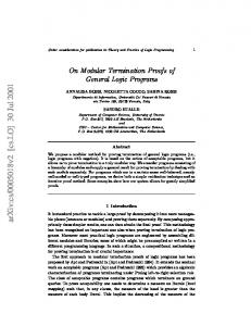
Termination provers for term rewrite systems (TRSs) became more and more powerful in the last years. One reason is that a proof of termination no longer is just some reduction order which contains the rewrite relation of the TRS. Currently, most provers construct a proof in the dependency pair framework which allows to combine basic termination techniques in a flexible way. Then a termination proof is a tree where at each node a specific technique has been applied. So instead of stating the precedence of some lexicographic path order (LPO) or giving some polynomial interpretation, current termination provers return proof trees which reach sizes of several megabytes. Hence, it would be too much work to check by hand whether these trees really form a valid proof. That we cannot blindly trust the output of termination provers is regularly demonstrated: Every now and then some tool delivers a faulty proof for some TRS. But most often this is only detected if there is some other prover giving the opposite answer on the same TRS, i.e., that it is nonterminating. To solve this problem, in the last years two systems have been developed which automatically certify or reject a generated termination proof: CiME/Coccinelle [4,6] and Rainbow/CoLoR [3] where Coccinelle and CoLoR are libraries on rewriting for Coq (http://coq.inria.fr), and CiME and Rainbow are used to convert proof trees into Coq-proofs which heavily rely on the theorems within those libraries. ?

This research is supported by FWF (Austrian Science Fund) project P18763.

CiME/Rainbow proof tree

Coq + Coccinelle/CoLoR proof.v

accept/failure

In this paper we present a new combination, CeTA/IsaFoR, to automatically certify termination proofs. Note that the system design has two major differences in comparison to the two existing ones. First, our library IsaFoR (Isabelle Formalization of Rewriting, containing 173 definitions, 863 theorems, and 269 functions) is written for the theorem prover Isabelle/HOL1 [16] and not for Coq. Second, and more important, instead of generating for each proof tree a new Coq-proof using the auxiliary tools CiME/Rainbow, our library IsaFoR contains several executable “check”-functions (within Isabelle) for each termination technique we formalized. We have formally proven that whenever such a check is accepted, then the termination technique is applied correctly. Hence, we do not need to create an individual Isabelle-proof for each proof tree, but just call the “check”-function for checking the whole tree (which does nothing else but calling the separate checks for each termination technique occurring in the tree). This second difference has several advantages: • In the other two systems, whenever a proof is not accepted, the user just gets a Coq-error message that some step in the generated Coq-proof failed. In contrast, our functions deliver error messages using notions of term rewriting. • Since the analysis of the proof trees in IsaFoR is performed by executable functions, we can just apply Isabelle’s code-generator [11] to create a certified Haskell program [17], CeTA, leading to the following workflow. IsaFoR proof tree

Isabelle CeTA

Haskell program

Haskell compiler CeTA

accept/error message

Hence, to use our certifier CeTA (Certified Termination Analysis) you do not have to install any theorem prover, but just execute some binary. Moreover, the runtime of certification is reduced significantly. Whereas the other two approaches take more than one hour to certify all (≤ 580) proofs during the last certified termination competition, CeTA needs less than two minutes for all (786) proofs that it can handle. Note that CeTA can also be used for modular certification. Each single application of a termination technique can be certified—just call the corresponding Haskell-function. Concerning the techniques that have been formalized, the other two systems offer techniques that are not present in IsaFoR, e.g., LPO or matrix interpretations. Nevertheless, we also feature one new technique that has not been certified so far. Whereas currently only the initial dependency graph estimation of [1] has been certified, we integrated the most powerful estimation which does not require tree automata techniques and is based on a combination of [9,12] where the function tcap is required. Initial problems in the formalization of tcap led to the development of etcap, an equivalent but more efficient version of tcap which 1

In the remainder of this paper we just write Isabelle instead of Isabelle/HOL.

2

is also beneficial for termination provers. Replacing tcap by etcap within the termination prover TTT2 [14] reduced the time to estimate the dependency graph by a factor of 2. We will also explain, how to reduce the number of edges that have to be inspected when checking graph decompositions. Another benefit of our system is its robustness. Every proof which uses weaker techniques than those formalized in IsaFoR is accepted. For example, termination provers can use the graph estimation of [1], as it is subsumed by our estimation. The paper is structured as follows. In Sect. 2 we recapitulate the required notions and notations of term rewriting and the dependency pair framework (DP framework). Here, we also introduce our formalization of term rewriting within IsaFoR. In Sect. 3–6 we explain our certification of the four termination techniques we currently support: dependency pairs (Sect. 3), dependency graph (Sect. 4), reduction pairs (Sect. 5), and combination of proofs in the dependency pair framework (Sect. 6). However, to increase readability we abstract from our concrete Isabelle code and present the checks for the techniques on a higher level. How we achieved readable error-messages while at the same time having maintainable Isabelle proofs is the topic of Sect. 7. We conclude in Sect. 8 where we show how CeTA is created from IsaFoR and where we give experimental data. IsaFoR, CeTA, and all details about our experiments are available at CeTA’s website http://cl-informatik.uibk.ac.at/software/ceta.

2

Formalizing Term Rewriting

We assume some basic knowledge of term rewriting [2]. Variables are denoted by x, y, z, etc., function symbols by f , g, h, etc., terms by s, t, u, etc., and substitutions by σ, µ, etc. Instead of f (t1 , . . . , tn ) we write f (tn ). The set of all variables occurring in term t is denoted by Var(t). By T (F, V) we denote the set of terms over function symbols from F and variables from V. In the following we give an overview of our formalization of term rewriting in IsaFoR. Our main concern is termination of rewriting. This property—also known as strong normalization—can be stated without considering the structure of terms. Therefore it is part of our Isabelle theory AbstractRewriting. An abstract rewrite system (ARS) is represented by the type (’a×’a)set in Isabelle. Strong normalization (SN) of a given ARS A is equivalent to the absence of an infinite sequence of A-steps. On the lowest level we have to link our notion of strong normalization to the notion of well-foundedness as defined in Isabelle. This is an easy lemma since the only difference is the orientation of the relation, i.e., SN(A) = wf(A−1 ). At this point we can be sure that our notion of strong normalization is valid. Now we come to the level of first-order terms (in theory Term):

datatype (’f,’v)"term" = Var ’v | Fun ’f "(’f,’v)term list" Many concepts related to terms are formalized in Term, e.g., an induction scheme for terms (as used in textbooks), substitutions, contexts, the (proper) subterm relation etc. By restricting the elements of some ARS to terms, we reach the level of TRSs 3

(in theory Trs), which in our formalization are just binary relations over terms. Example 1. As an example, consider the following TRS, encoding rules for subtraction and division on natural numbers. minus(x, 0) → x

div(0, s(y)) → 0

minus(s(x), s(y)) → minus(x, y)

div(s(x), s(y)) → s(div(minus(x, y), s(y)))

Given a TRS R, (`, r) ∈ R means that ` is the lhs and r the rhs of a rule in R (usually written as ` → r ∈ R). The rewrite relation induced by a TRS R is denoted by →R and has the following definition in IsaFoR: Definition 2. Term s rewrites to t by R, iff there are a context C, a substitution σ, and a rule ` → r ∈ R such that s = C[`σ] and t = C[rσ]. Note that this section contains the only parts where you have to trust our formalization, i.e., you have to believe that SN(→R ) as defined in IsaFoR really describes “R is terminating.”

3

Certifying Dependency Pairs

Before we introduce dependency pairs [1] formally and give some details about our Isabelle formalization, we recapitulate the ideas that led to the final definition (including a refinement proposed by Dershowitz [7]). For a TRS R, strong normalization means that there is no infinite derivation t1 →R t2 →R t3 →R · · · . Additionally we can concentrate on derivations, where t1 is minimal in the sense that all its proper subterms are terminating. Such terms are called minimal nonterminating. The set of all minimally nonterminating terms with respect to a TRS R is denoted by TR∞ . Observe that for every term t ∈ TR∞ there is an initial part of an infinite derivation having a specific shape: A (possibly empty) derivation taking place below the root, followed by an >ε∗ ε application of some rule ` → r ∈ R at the root, i.e., t →R `σ →R rσ, for some substitution σ. Furthermore, since rσ is nonterminating, there is some subterm u of r, such that uσ ∈ TR∞ , i.e., rσ = C[uσ]. Then the same reasoning can be used to get a root reduction of uσ, . . . , cf. [1]. To get rid of the additional contexts C a new TRS, DP(R), is built. Definition 3. The set DP(R) of dependency pairs of R is defined as follows: For every rule ` → r ∈ R, and every subterm u of r such that u is not a proper subterm of ` and such that the root of u is defined,2 `] → u] is contained in DP(R). Here t] is the same as t except that the root of t is marked with the special symbol ]. Example 4. The dependency pairs for the TRS from Ex. 1 consist of the rules M(s(x), s(y)) → M(x, y) (MM)

D(s(x), s(y)) → M(x, y)

(DM)

D(s(x), s(y)) → D(minus(x, y), s(y)) (DD) where we write M instead of minus and D instead of div] for brevity. ]

2

A function symbol f is defined (w.r.t. R) if there is some rule f (. . . ) → r ∈ R.

4

Note that after switching to ’]’-terms, the derivation from above can be written as t] →∗R `] σ →DP(R) u] σ. Hence every nonterminating derivation starting at a term t ∈ TR∞ can be transformed into an infinite derivation of the following shape where all →DP(R) -steps are applied at the root. t] →∗R s]1 →DP(R) t]1 →∗R s]2 →DP(R) t]2 →∗R · · ·

(1)

Therefore, to prove termination of R it suffices to prove that there is no such derivation. To formalize DPs in Isabelle we modify the signature such that every function symbol now appears in a plain version and in a ]-version.

datatype ’f shp = Sharp ’f ("_]") | Plain ’f ("_@") Sharping a term is done via

fun plain :: "(’f,’v)term => (’f shp,’v)term" where "plain(Var x) = Var x" | "plain(Fun f ss) = Fun f@ (map plain ss)"

fun sharp :: "(’f,’v)term => (’f shp,’v)term" where "sharp(Var x) = Var x" | "sharp(Fun f ss) = Fun f] (map plain ss)" Thus t] in Def. 3 is the same as sharp(t). Since the function symbols in DP(R) are of type ’f shp and the function symbols of R are of type ’f, it is not possible to use the same TRS R in combination with DP(R). Thus, in our formalization we use the lifting ID—that just applies plain to all lhss and rhss in R. Considering this technicalities and omitting the initial derivation t] →∗R s]1 from the derivation (1), we obtain s]1 →DP(R) t]1 →∗ID(R) s]2 →DP(R) t]2 →∗ID(R) · · · and hence a so called infinite (DP(R), ID(R))-chain. Then the corresponding DP problem (DP(R), ID(R)) is called to be not finite, cf. [8]. Notice that in IsaFoR a DP problem is just a pair of two TRSs over arbitrary signatures—similar to [8]. In IsaFoR an infinite chain3 and finite DP problems are defined as follows.

fun ichain where "ichain(P, R) s t σ = (∀i.

(s i,t i) ∈ P ∧ (t i)·(σ i) →∗R (s(i+1))·(σ(i+1))"

fun finite_dpp where "finite_dpp(P, R) = (¬(∃s t σ. ichain (P, R) s t σ))" where ‘t · σ’ denotes the application of substitution σ to term t. We formally established the connection between strong normalization and finiteness of the initial DP problem (DP(R), ID(R)). Although this is a wellknown theorem, formalizing it in Isabelle was a major effort. Theorem 5. wf_trs(R) ∧ finite_dpp(DP(R), ID(R)) −→ SN(→R ). 3

We also formalized minimal chains, but here only present chains for simplicity.

5

The additional premise wf_trs(R) ensures two well-formedness properties for R, namely that for every ` → r ∈ R, ` is not a variable and that Var(r) ⊆ Var(`). At this point we can obviously switch from the problem of proving SN(→R ) for some TRS R, to the problem of proving finite_dpp(DP(R), ID(R)), and thus enter the realm of the DP framework [8]. Here, the current technique is to apply so-called processors to a DP problem, in order to get a set of simpler DP problems. This is done recursively, until the leafs of the so built tree consist of DP problems with empty P-components (and therefore are trivially finite). For this to be correct, the applied processors need to be sound, i.e., every processor P roc has to satisfy the implication (∀p ∈ P roc(P, R). finite_dpp(p)) −→ finite_dpp(P, R) for every input. The termination techniques that will be introduced in the following sections are all such (sound) processors. So much to the underlying formalization. Now we will present how the check in IsaFoR certifies a set of DPs P that was generated by some termination tool for some TRS R. To this end, the function checkDPs is used. checkDPs(P,R) = checkWfTRS(R) ∧ computeDPs(R) ⊆ P Here checkWfTRS checks the two well-formedness properties mentioned above (the difference between wf_trs and checkWfTRS is that only the latter is executable) and computeDPs uses Def. 3, which is currently the strongest definition of DPs. To have a robust system, the check does not require that exactly the set of DPs w.r.t. to Def. 3 is provided, but any superset is accepted. Hence we are also able to accept proofs from termination tools that use a weaker definition of DP(R). The soundness result of checkDPs is formulated as follows in IsaFoR. Theorem 6. If checkDPs(P, R) is accepted then finiteness of (P, ID(R)) implies SN(→R ).

4

Certifying the Dependency Graph Processor

One important processor to prove finiteness of a DP problem is based on the dependency graph [1,8]. The dependency graph of a DP problem (P, R) is a directed graph G = (P, E) where (s → t, u → v) ∈ E iff s → t, u → v is a (P, R)-chain. Hence, every infinite (P, R)-chain corresponds to an infinite path in G and thus, must end in some strongly connected component (SCC) S of G, provided that P contains only finitely many DPs. Dropping the initial DPs of the chain results in an infinite (S, R)-chain.4 Hence, if for all SCCs S of G the DP problem (S, R) is finite, then (P, R) is finite. In practice, this processor allows to prove termination of each block of mutual recursive functions separately. To certify an application of the dependency graph processor there are two main challenges. First of all, we have to certify that a valid SCC decomposition of G is used, a purely graph-theoretical problem. Second, we have to generate the edges of G. Since the dependency graph G is in general not computable, usually 4

We identify an SCC S with the set of nodes S within that SCC.

6

estimated graphs G 0 are used which contain all edges of the real dependency graph G. Hence, for the second problem we have to implement and certify one estimation of the dependency graph. Notice that there are various estimations around and that the result of an SCC decomposition depends on the estimation that is used. Hence, it is not a good idea to implement the strongest estimation and then match the result of our decomposition against some given decomposition: problems arise if the termination prover used a weaker estimation and thus obtained larger SCCs. Therefore, in the upcoming Sect. 4.1 about graph algorithms we just speak of decompositions where the components do not have to be SCCs. Moreover, we will also elaborate on how to minimize the number of tests (s → t, u → v) ∈ E. The reason is that in Sect. 4.2 we implemented one of the strongest dependency graph estimations where the test for an edge can become expensive. In Sect. 4.3 we finally show how to combine the results of Sections 4.1 and 4.2. 4.1

Certifying Graph Decompositions

Instead of doing an SCC decomposition of a graph within IsaFoR we base our check on the decomposition that is provided by the termination prover. Essentially, we demand that the set of components is given as a list hC1 , . . . , Ck i in topological order where the component with no incoming edges is listed first. Then we aim at certifying that every infinite path must end in some Ci . Note that the general idea of taking the topological sorted list as input was already publicly mentioned at the “Workshop on the certification of termination proofs” in 2007. In the following we present how we filled the details of this general idea. The main idea is to ensure that all edges (p, q) ∈ E correspond to a step forward in the list hC1 , . . . , Ck i, i.e., (p, q) ∈ Ci × Cj where i ≤ j. However, iterating over all edges of G will be costly, because it requires to perform the test (p, q) ∈ E for all possible edges (p, q) ∈ P × P. To overcome this problem we do not iterate over the edges but over P. To be more precise, we check that ∀(p, q) ∈ P × P. (∃i ≤ j. (p, q) ∈ Pi × Pj ) ∨ (p, q) ∈ /E

(2)

where the latter part of the disjunction is computed only on demand. Thus, only those edges have to be computed, which would contradict a valid decomposition. Example 7. Consider the set of nodes P = {(DD), (DM), (MM)}. Suppose that we have to check a decomposition of P into L = h{(DD)}, {(DM)}, {(MM)}i for some graph G = (P, E). Then our check has to ensure that the dashed edges in the following illustration do not belong to E. (DD)

(DM)

(MM)

It is easy to see that (2) is satisfied for every list of SCCs that is given in topological order. What is even more important, whenever there is a valid SCC decomposition of G, then (2) is also satisfied for every subgraph. Hence, regardless of the dependency graph estimation a termination prover might have used, we accept it, as long as our estimation delivers less edges. 7

However, the criterion is still too relaxed, since we might cheat in the input by listing nodes twice. Consider P = {p1 , . . . , pm } where the corresponding graph is arbitrary and L = h{p1 }, . . . , {pm }, {p1 }, . . . , {pm }i. Then trivially (2) is satisfied, because we can always take the source of edge (pi , pj ) from the first part of L and the target from the second part of L. To prevent this kind of problem, our criterion demands that the sets Ci in L are pairwise disjoint. Before we formally state our theorem, there is one last step to consider, namely the handling of singleton nodes which do not form an SCC on their own. Since we cannot easily infer at what position these nodes have to be inserted in the topological sorted list—this would amount to do an SCC decomposition on our own—we demand that they are contained in the list of components.5 To distinguish a singleton node without an edge to itself from a “real SCC”, we require that the latter ones are marked. Then condition (2) is extended in a way that unmarked components may have no edge to themselves. The advantage of not marking a component is that our IsaFoR-theorem about graph decomposition states that every infinite path will end in some marked component, i.e., here the unmarked components can be ignored. Theorem 8. Let L = hC1 , . . . , Ck i be a list of sets of nodes, some of them marked, let G = (P, E) be a graph, let α be an infinite path of G. If • ∀(p, q) ∈ P × P. (∃i < j. (p, q) ∈ Ci × Cj ) ∨ (∃i. (p, q) ∈ Ci × Ci ∧ Ci is marked) ∨ (p, q) ∈ /E and • ∀i 6= j. Ci ∩ Cj = ∅ then there is some suffix β of α and some marked Ci such that all nodes of β belong to Ci . Example 9. If we continue with example Ex. 7 where only components {(MM)} and {(DD)} are marked, then our check also analyzes that G contains no edge from (DM) to itself. If it succeeds, every infinite path will in the end only contain nodes from {(DD)} or only nodes from {(MM)}. In this way, only 4 edges of G have to be calculated instead of analyzing all 9 possible edges in P × P. 4.2

Certifying Dependency Graph Estimations

What is currently missing to certify an application of the dependency graph processor, is to check, whether a singleton edge is in the dependency graph or not. Hence, we have to estimate whether the sequence s → t, u → v is a chain, i.e., whether there are substitutions σ and µ such that tσ →∗R uµ. An obvious solution is to just look at the root symbols of t and u—if they are different there is no way that the above condition is met (since all the steps in tσ →∗R uµ take place below the root, by construction of the dependency pairs). Although efficient and often good enough, there are more advanced estimations around. The estimation EDG [1] first replaces via an operation cap all variables and all subterms of t which have a defined root-symbol by distinct fresh variables. Then if cap(t) and u do not unify, it is guaranteed that there is no edge. 5

Note that Tarjan’s SCC decomposition algorithm produces exactly this list.

8

The estimation EDG∗ [12] does the same check and additionally uses the reversed TRS R−1 = {r → ` | ` → r ∈ R}, i.e., it uses the fact that tσ →∗R uµ implies uµ →∗R−1 tσ and checks whether cap(u) does not unify with t. Of course in the application of cap(u) we have to take the reversed rules into account (possibly changing the set of defined symbols) and it is not applicable if R contains a collapsing rule ` → x where x ∈ V. The last estimation we consider is based on a better version of cap, called tcap [9]. It only replaces subterms with defined symbols by a fresh variable, if there is a rule that unifies with the corresponding subterm. Definition 10. Let R be a TRS. • tcap(f (tn )) = f (tcap(t1 ), . . . , tcap(tn )) iff f (tcap(t1 ), . . . , tcap(tn )) does not unify with any variable renamed left-hand side of a rule from R • tcap(t) is a fresh variable, otherwise To illustrate the difference between cap and tcap consider the TRS of Ex. 1 and t = div(0, 0). Then cap(t) = xfresh since div is a defined symbol. However, tcap(t) = t since there is no division rule where the second argument is 0. Apart from tree automata techniques, currently the most powerful estimation is the one based on tcap looking both forward as in EDG and backward as in EDG∗ . Hence, we aimed to implement and certify this estimation in IsaFoR. Unfortunately, when doing so, we had a problem with the domain of variables. The problem was that although we first implemented and certified the standard unification algorithm of [15], we could not directly apply it to compute tcap. The reason is that to generate fresh variables as well as to rename variables in rules apart, we need a type of variables with an infinite domain. One solution would have been to constrain the type of variables where there is a function which delivers a fresh variable w.r.t. any given finite set of variables. However, there is another and more efficient approach to deal with this problem than the standard approach to rename and then do unification. Our solution is to switch to another kind of terms where instead of variables there is just one special constructor “” representing an arbitrary fresh variable. In essence, this data structure represents contexts which do not contain variables, but where multiple holes are allowed. Therefore in the following we speak of ground-contexts and use C, D, . . . to denote them. Definition 11. Let JCK be the equivalence class of a ground-context C where the holes are filled with arbitrary terms: JCK = {C[t1 , . . . , tn ] | t1 , . . . , tn ∈ T (F, V)}. Obviously, every ground-context C can be turned into a term t which only contains distinct fresh variables and vice-versa. Moreover, every unification problem between t and ` can be formulated as a ground-context matching problem between C and `, which is satisfiable iff there is some µ such that `µ ∈ JCK. Since the result of tcap is always a term which only contains distinct fresh variables, we can do the computation of tcap using the data structure of groundcontexts; it only requires an algorithm for ground-context matching. To this end we first generalize ground-context matching problems to multiple pairs (Ci , `i ). 9

Definition 12. A ground-context matching problem is a set of pairs M = {(C1 , `1 ), . . . , (Cn , `n )}. It is solvable iff there is some µ such that `i µ ∈ JCi K for all 1 ≤ i ≤ n. We sometimes abbreviate {(C, `)} by (C, `). To decide ground-context matching we devised a specialized algorithm which is similar to standard unification algorithms, but which has some advantages: it does neither require occur-checks as the unification algorithm, nor is it necessary to preprocess the left-hand sides of rules by renaming (as would be necessary for standard tcap). And instead of applying substitutions on variables, we just need a basic operation on ground-contexts called merge such that merge(C, D) = ⊥ implies JCK ∩ JDK = ∅, and merge(C, D) = E implies JCK ∩ JDK = JEK. Definition 13. The following rules simplify a ground-context matching problem into solved form (where all terms are distinct variables) or into ⊥. (a) (b) (c) (d) (e)

M ∪ {(, `)} M ∪ {(f (D n ), f (un ))} M ∪ {(f (D n ), g(uk ))} M ∪ {(C, x), (D, x)} M ∪ {(C, x), (D, x)}

⇒match ⇒match ⇒match ⇒match ⇒match

M M ∪ {(D1 , u1 ), . . . , (Dn , un )} ⊥ if f 6= g or n 6= k M ∪ {(E, x)} if merge(C, D) = E ⊥ if merge(C, D) = ⊥

Rules (a–c) obviously preserve solvability of M (where ⊥ represents an unsolvable matching problem). For Rules (d,e) we argue as follows: • • • •

{(C, x), (D, x)} ∪ . . . is solvable iff there is some µ such that xµ ∈ JCK and xµ ∈ JDK and . . . iff there is some µ such that xµ ∈ JCK ∩ JDK and . . . iff there is some µ such that xµ ∈ Jmerge(C, D)K and . . . iff {(merge(C, D), x)} ∪ . . . is solvable

Since every ground-context matching problem in solved form is solvable, we have devised a decision procedure. It can be implemented in two stages where the first stage just normalizes by the Rules (a–c), and the second stage just applies the Rules (d,e). It remains to implement merge. merge(, C) ⇒merge C merge(C, ) ⇒merge C merge(f (C n ), g(D k )) ⇒merge ⊥

if f 6= g or n 6= k

merge(f (C n ), f (D n )) ⇒merge f (merge(C1 , D1 ), . . . , merge(Cn , Dn )) f (. . . , ⊥, . . .) ⇒merge ⊥ Note that our implementations of the matching algorithm and the merge function in IsaFoR are slightly different due to different data structures. For example matching problems are represented as lists of pairs, so it may occur that we have duplicates in M. The details of our implementation can be seen in IsaFoR (theory Edg) or in the source of CeTA. 10

Soundness and completeness of our algorithms are proven in IsaFoR. Theorem 14. • If merge(C, D) ⇒∗merge ⊥ then JCK ∩ JDK = ∅. • If merge(C, D) ⇒∗merge E then JCK ∩ JDK = JEK. • If (C, `) ⇒∗match ⊥ then there is no µ such that `µ ∈ JCK. • If (C, `) ⇒∗match M where M is in solved form, then there exists some µ such that `µ ∈ JCK.

Using ⇒match , we can now easily reformulate tcap in terms of ground-context matching which results in the efficient implementation etcap. Definition 15. • etcap(f (tn )) = f (etcap(t1 ), . . . , etcap(tn )) iff (f (etcap(t1 ), . . . , etcap(tn )), `) ⇒∗match ⊥ for all rules ` → r ∈ R. • , otherwise One can also reformulate the desired check to estimate the dependency graph whether tcap(t) does not unify with u in terms of etcap. It is the same requirement as demanding (etcap(t), u) ⇒∗match ⊥. Again, the soundness of this estimation has been proven in IsaFoR where the second part of the theorem is a direct consequence of the first part by using the soundness of the matching algorithm. Theorem 16. (a) Whenever tσ →∗R s then s ∈ Jetcap(t)K. (b) Whenever tσ →∗R uτ then (etcap(t), u) 6⇒∗match ⊥ and (etcap(u), t) 6⇒∗match ⊥ where etcap(u) is computed w.r.t. the reversed TRS R−1 . 4.3

Certifying Dependency Graph Decomposition

Eventually we can connect the results of the previous two subsections to obtain one function to check a valid application of the dependency graph processor. checkDepGraphProc(P, L, R) = checkDecomposition(checkEdg(R), P, L) where checkEdg just applies the criterion of Thm. 16 (b). In IsaFoR the soundness result of our check is proven. Theorem 17. If checkDepGraphProc(P, L, R) is accepted and if for all P 0 ∈ L where P 0 is marked, the DP problem (P 0 , R) is finite, then (P, R) is finite. To summarize, we have implemented and certified the currently best dependency graph estimation which does not use tree automata techniques. Our check-function accepts any decomposition which is based on a weaker estimation, but requires that the components are given in topological order. Since our algorithm computes edges only on demand, the number of tests for an edge is reduced considerably. For example, the five largest graphs in our experiments contain 73,100 potential edges, but our algorithm only has to consider 31,266. This reduced the number of matchings from 13 millions down to 4 millions. Furthermore, our problem of not being able to generate fresh variables or to rename variables in rules apart led to a more efficient algorithm for tcap based on matching instead of unification: simply replacing tcap by etcap in TTT2 reduced the time for estimating the dependency graph by a factor of two. 11

5

Certifying the Reduction Pair Processor

One important technique to prove finiteness of a DP problem (P, R) is the socalled reduction pair processor. The general idea is to use a well-founded order where all rules of P ∪ R are weakly decreasing. Then we can delete all strictly decreasing rules from P and continue with the remaining dependency pairs. We first state a simplified version of the reduction pair processor as it is introduced in [8], where we ignore the usable rules refinement. Theorem 18. If all the following properties are satisfied, then finiteness of (P \ , R) implies finiteness of (P, R). (a) (b) (c) (d)

 is a well-founded and stable order % is a stable and monotone quasi-order % ◦  ⊆  and  ◦ % ⊆  P ⊆  ∪ % and R ⊆ %

Of course, to instantiate the reduction pair processor with a new kind of reduction pair, e.g., LPO, polynomial orders,. . . , we first have to prove the first three properties for that kind of reduction pairs. Since we plan to integrate many reduction pairs, but only want to write the reduction pair processor once, we tried to minimize these basic requirements such that the reduction pair processor still remains sound in total. In the end, we replaced the first three properties by: (a)  is a well-founded and stable relation (b) % is a stable and monotone relation (c) % ◦  ⊆  In this way, for every new class of reduction pairs, we do not have to prove transitivity of  or % anymore, as it would be required for Thm. 18. Currently, we just support reduction pairs based on polynomial interpretations with negative constants [13], but we plan to integrate other reduction pairs in the future. For checking an application of a reduction pair processor we implemented a generic function checkRedPairProc in Isabelle, which works as follows. It takes as input two functions checkS and checkNS which have to approximate a reduction pair, i.e., whenever checkS(s, t) is accepted, then s  t must hold in the corresponding reduction pair and similarly, checkNS has to guarantee s % t. Then checkRedPairProc(checkS, checkNS, P, P 0 , R) works as follows: • iterate once over P to divide P into P and P6 where the former set contains all pairs of P where checkS is accepted • ensure for all s → t ∈ R ∪ P6 that checkNS(s, t) is accepted, otherwise reject • accept if P6 ⊆ P 0 , otherwise reject The corresponding theorem in IsaFoR states that a successful application of checkRedPairProc(. . . , P, P 0 , R) proves that (P, R) is finite whenever (P 0 , R) is finite. Obviously, the first two conditions of checkRedPairProc ensure condition (d) of Thm. 18. Note, that it is not required that all strictly decreasing pairs are removed, i.e., our checks may be stronger than the ones that have been used in the termination provers. 12

6

Certifying the Whole Proof Tree

From Sect. 3–5 we have basic checks for the three techniques of applying dependency pairs (checkDPs), the dependency graph processor (checkDepGraphProc), and the reduction pair processor (checkRedPairProc). For representing proof trees within the DP framework we used the following data structures in IsaFoR.

datatype ’f RedPair = NegPolo "(’f × (cint × nat list))list" datatype (’f,’v)DPProof = . . . 6 | PisEmpty | RedPairProc "’f RedPair" "(’f,’v)trsL" "(’f,’v)DPProof" | DepGraphProc "((’f,’v)DPProof option × (’f,’v)trsL)list"

datatype (’f,’v)TRSProof = . . . 6 | DPTrans "(’f shp,’v)trsL" "(’f shp,’v)DPProof" The first line fixes the format for reduction pairs, i.e., currently of (linear) polynomial interpretations where for every symbol there is one corresponding entry. E.g., the list [(f, (−2, [0, 3]))] represents the interpretation where Pol(f )(x, y) = max(−2 + 3y, 0) and Pol(g)(x1 , . . . , xn ) = 1 + Σ1≤i≤n xi for all f 6= g. The datatype DPProof represents proof trees for DP problems. Then the check for valid DPProofs gets as input a DP problem (P, R) and a proof tree and tries to certify that (P, R) is finite. The most basic technique is the one called PisEmpty, which demands that the set P is empty. Then (P, R) is trivially finite. For an application of the reduction pair processor, three inputs are required. First, the reduction pair redp, i.e., some polynomial interpretation. Second, the dependency pairs P 0 that remain after the application of the reduction pair processor. Here, the datatype trsL is an abbreviation for lists of rules. And third, a proof that the remaining DP problem (P 0 , R) is finite. Then the checker just has to call createRedPairProc(redp, P, P 0 , R) and additionally calls itself recursively on (P 0 , R). Here, createRedPairProc invokes checkRedPairProc where checkS and checkNS are generated from redp. The most complex structure is the one for decomposition of the (estimated) dependency graph. Here, the topological list for the decomposition has to be provided. Moreover, for each subproblem P 0 , there is an optional proof tree. Subproblems where a proof is given are interpreted as “real SCCs” whereas the ones without proof remain unmarked for the function checkDepGraphProc. The overall function for checking proof trees for DP problems looks as follows. checkDPProof(P,R,PisEmpty) = (P = []) checkDPProof(P,R,(RedPairProc redp P 0 prf)) = createRedPairProc(redp,P,P 0 ,R) ∧ checkDP(P 0 ,R,prf) checkDPProof(P,R,DepGraphProc P 0 s) = checkDepGraphProc(P,map (λ(prfO,P 0 ).(isSome prfO,P 0 )) P 0 s, R) V ∧ (Some prf,P 0 )∈P 0 s checkDPProof(P 0 ,R,prf) 6

CeTA supports even more techniques, cf. CeTA’s website for a complete list.

13

Theorem 19. If checkDPProof(P,R,prf) is accepted then (P, R) is finite. Using checkDPProof it is now easy to write the final method checkTRSProof for proving termination of a TRS, where computeID is an implementation of ID. checkTRSProof(R,DPTrans P prf) = checkDPs(R,P) ∧ checkDPProof(P,computeID(R),prf) For the external usage of CeTA we developed a well documented XML-format, cf. CeTA’s website. Moreover, we implemented two XML parsers in Isabelle, one that transforms a given TRS into the internal format, and another that does the same for a given proof. The function certifyProof, finally, puts everything together. As input it takes two strings (a TRS and its proof). Then it applies the mentioned parsers and afterwards calls checkTRSProof on the result. Theorem 20. If certifyProof(R,prf) is accepted then SN(→R ). To ensure that the parser produces the right TRS, after the parsing process it is checked that when converting the internal data-structures of the TRS back to XML, we get the same string as the input string for the TRS (modulo whitespace). This is a major benefit in comparison to the two other approaches where it can and already has happened that the uncertified components Rainbow/CiME produced a wrong proof goal from the input TRS, i.e., they created a termination proof within Coq for a different TRS than the input TRS.

7

Error Messages

To generate readable error messages, our checks do not have a Boolean return type, but a monadic one (isomorphic to ’e option). Here, None represents an accepted check whereas Some e represents a rejected check with error message e. The theory ErrorMonad contains several basic operations like >> for conjunction of checks,