Title: Automated tools within workflows for 3D structural construction from .... analysis of data, dip-domain construction, and 3D surface construction (Figure 1).
Editorial Manager(tm) for Geoinformatica Manuscript Draft
Manuscript Number: GEIN133R1 Title: Automated tools within workflows for 3D structural construction from surface and subsurface data Article Type: Special Issue: Geology and Info. Tech. Section/Category: Keywords: structural modeling; orientation analysis; dip-domain; isopach Corresponding Author: Dr. Oscar Fernandez, Corresponding Author's Institution: First Author: Oscar Fernandez Order of Authors: Oscar Fernandez; Serena Jones, Dr; Norman Armstrong; Gareth Johnson; Antonio Ravaglia, Dr; Josep Anton Muñoz, Prof Manuscript Region of Origin:
Cover Letter - Response to reviewers
Dear sirs, We have uploaded our revised manuscript and figures. Below you will find a list of the main changes we have made with respect to the comments made by the reviewers. Best regards, Oscar Fernandez
Reviewer #1 – 1) Modified text in the introduction to better define the areas of applicability of the techniques discussed in the paper 2) The section in the workflow describing the use of geological maps to obtain structural information has been expanded to include the reviewer’s concerns. The reviewer’s comments on the limitations of the technique are discussed in the section on the automated tool for dip calculation from geological contacts. This is precisely one of the novelties of the approach: whereas previous authors have used geological maps to obtain dip without any quantitative control on the quality of the measurement, we are providing a tool that includes a quantification of the quality as one of its main outputs. This quantification is meant to provide the user with an accurate way to evaluate the applicability of the tool to his/her particular case. 3) A 3D illustration has been used to replace Figure 6, as requested by the reviewer.
Reviewer #2 – The objective of this paper is to present a number of novel automatic tools that can be embedded into a workflow for 3D structural reconstruction. It is not our goal to automate the entire workflow and we consider that is well beyond the scope of this paper. The three tools discussed in the paper apply to three very particular problems encountered by geologists when attempting 3D reconstructions from outcrop and well data. The technique for automated dip calculations presented herein significantly improves the more standard 3-point approach now commonly used to obtain structural data in areas of limited accessibility. The 3D dip-domain surface construction is the first step in transforming one of the most powerful interpolation techniques in 2D cross-section construction into a 3D tool. Finally, 3D isopach measurement is an incredibly powerful tool for construction and analysis of 3D models, particularly given that to our knowledge the only alternative to the tool discussed are “manual” calculations.
Manuscript Click here to download Manuscript: Fernandez_et_al_2007_final.doc
1 2 3 4 5 6 7 8 9 10 11 12 13 14 15 16 17 18 19 20 21 22 23 24 25 26 27 28 29 30 31 32 33 34 35 36 37 38 39 40 41 42 43 44 45 46 47 48 49 50 51 52 53 54 55 56 57 58 59 60 61 62 63 64 65
Automated tools within workflows for 3D structural construction from surface and subsurface data O. Fernandez, S. Jones, N. Armstrong, G. Johnson, A. Ravaglia, J.A. Muñoz Abstract Mainstream techniques for the construction of 3D geological models frequently rely on high-density subsurface datasets, such as 3D seismic surveys or dense 2D seismic grids. In settings where the available geological and/or geophysical data are relatively sparse, the construction of a consistent 3D structural framework is seldom straightforward and is strongly dependent on the optimization of the use of surface data. To deal with this challenge, workflows for constructing 3D models from sparse surface data have been proposed by multiple authors. This paper presents three automated techniques which optimize the use of data and enhance the time-efficiency of 3D model construction: 3D geological contact analysis, 3D dip-domain construction, and 3D isopach measurement and construction.
Introduction In recent years, the construction of 3D structural models has become a prerequisite in both industry and academia-led projects. In areas of complex structure or of limited accessibility, as are onshore fold-and-thrust provinces, geological and geophysical data are often sparse, making the problem of 3D construction a non-trivial one. Over recent years, different authors have suggested approaches to optimize the 3D nature of surface (field) data in the construction of 3D models (e.g., [4], [5], [12], [11], [8], [6]). The goal of this article is to present three new automated tools inscribed in a general workflow for 3D construction based on that presented by [5]. These tools solve key issues present in structural analysis, initial surface construction and final 3D model construction steps of the workflow.
Workflow The workflow for 3D structural construction proposed by [5] is used as a framework for the development of the tools presented in this paper. This workflow integrates surface data to generate 3D reconstructions of geological surfaces through the process of detailed structural analysis of data, dip-domain construction, and 3D surface construction (Figure 1). Figure 1. Geological data are collected in the field (a) and georeferenced in 3D by acquiring the Z coordinate from DEM or equivalent digital topography (b). Dip data are analyzed to define dip-domains and geological contacts to obtain extra orientation measurements (c). A single key horizon is constructed by creating single surfaces of constant dip according to dip-domain and placed at the
Automated tools in 3D structural modeling
1 2 3 4 5 6 7 8 9 10 11 12 13 14 15 16 17 18 19 20 21 22 23 24 25 26 27 28 29 30 31 32 33 34 35 36 37 38 39 40 41 42 43 44 45 46 47 48 49 50 51 52 53 54 55 56 57 58 59 60 61 62 63 64 65
stratigraphic position of the key horizon by displacing them perpendicular to bedding (d). Neighboring dip-domain patches are intersected and tidied to generate a single surface.
The process starts with geo-referencing and digitizing data and attributes in 3D space (in the case of surface geology by locating data on topography) (Figure 1a,b). Depending on the type of data, it can be analyzed to obtain different information. Dip data can be analyzed to define dip-domains (sectors where bedding orientation is approximately constant), their areal extent, and the position and nature of their boundaries (e.g., axial surfaces, faults, unconformities) (Figure 1c). Geological mapping can be analyzed to obtain the local dip of geological surfaces (Figure 1c). Due to their areal extent, geometrical analysis of geological contacts provides a measure of the orientation of geological surfaces that is more regional than that indicated by individual field dip measurements. This is particularly true when there isn’t an accurate control on the quality of field dip measurements, such as uncertainties on whether the dip was measured at the base of a channel or on a cross-bedding surface because of outcrop limitations. In these instances, geological contacts at the map scale will provide a better estimate of bedding, unless the contact is an unconformity (which should be easily identifiable at map scale), Furthermore, geological contacts also provide a better constraint on defining the lateral variations in the geometry (as in folding) of geological surfaces than sparsely distributed field dip measurements. Evidently, the technique of extracting structural information from geological mapping depends on the quality of mapping and the presence of sufficient topographical ruggedness, as will be discussed in the next section. The complete 3D geometrical analysis of data is then used to create partial 3D surfaces honouring local dip-domain orientations (we call these partial constructions 3D patches) (Figure 1d). 3D patch construction is aimed at generating a key horizon that can be used as a template for constructing new horizons. Data that lies on this key horizon (dips on the key horizon or geological contact of that horizon) can be used to create 3D patches that are already defining a part of the key horizon. Data that does not lie on the key horizon can be projected stratigraphically (translated perpendicular to bedding) until it lies on the desired horizon. All 3D patches lying on a single stratigraphic horizon are then merged to create complete 3D surfaces (Figure 1d). The construction of a complete 3D model requires the construction of multiple 3D horizons and any bounding faults. The process of constructing multiple horizons is also used to confirm the quality of the 3D analysis and construction. The construction of faults can follow the same procedure as that used for the construction of stratigraphic horizons if they are being constructed from similar data (field and subsurface data with the position and orientation of the fault surface). Once a complete 3D model has been obtained it can be used for further
Automated tools in 3D structural modeling
1 2 3 4 5 6 7 8 9 10 11 12 13 14 15 16 17 18 19 20 21 22 23 24 25 26 27 28 29 30 31 32 33 34 35 36 37 38 39 40 41 42 43 44 45 46 47 48 49 50 51 52 53 54 55 56 57 58 59 60 61 62 63 64 65
analysis, including restoration, geometrical analysis, and even the generation of representative cross-sections.
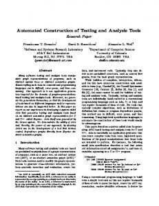
Automated tools In this paper we present three tools that automate three different procedures that are an integral part of the workflow discussed above. The first tool makes it possible to automatically extract structural orientation information from a geological contact and construct 3D surfaces along contacts. The second tool is an advance in dip-domain construction that allows construction of neighboring dip-domain surfaces and the definition of dip-domain axial surfaces. Finally, a third tool that permits the automated construction of multiple horizons once a key horizon has been built, greatly enhances the population of the complete 3D model. Geological contact analysis In the 3D construction workflow the analysis of geological contacts is done following the approach proposed by [9] based on moment-of-inertia analysis [14]. This approach is based on the principle that any geological contact results from the intersection of a geological surface with topography. In the presence of topography, the contact line will define upright and inverted ‘V’ shapes as it crosses valleys and ridges respectively. Wherever the geometry of the contact defines a ‘V’ shape, the position of digitized nodes along the contact can be used to provide information on the structural orientation (strike and dip) of the geological surface. Even though V’s are the ideal geometry to obtain dip from a geological contact, this technique does not require the contact to be mapped continuously, and can actually be a collection of discontinuously mapped segments. As opposed to the more traditional 3 point problem, the moment-of-inertia analysis approach uses multiple digitized nodes in its calculation of the orientation of the geological surface and therefore provides a measure less prone to spurious errors related to sampling. Other authors ([2], [3], [1]) have proposed using the planar regression of geological contacts,also using multiple nodes, with the same objective of providing more statistically valid results. However, the advantage of the moment-of-inertia analysis approach is that it yields two measures of the reliability or quality of the average orientation calculated. These two measures correspond to ratios of the eigenvalues [14]. One of the ratios (ratio K) indicates the degree of colinearity of the segment of contact analysed. On straight segments (such as along a flat valley bottom) the value of K will increase, whereas in segments where the contact turns around a ridge or a narrow valley, it will decrease, indicating a better defined ‘V’ shape. Measurements in areas of low K indicate higher topographic surface ruggedness and are therefore more reliable (Figure 2a). The second ratio (ratio M) is an indicator of the coplanarity of the segment of contact
Automated tools in 3D structural modeling
1 2 3 4 5 6 7 8 9 10 11 12 13 14 15 16 17 18 19 20 21 22 23 24 25 26 27 28 29 30 31 32 33 34 35 36 37 38 39 40 41 42 43 44 45 46 47 48 49 50 51 52 53 54 55 56 57 58 59 60 61 62 63 64 65
analysed. If orientation of the contact varies along strike (e.g., due to folding or erosional character of the contact) or the contact is not digitized properly due to poor correlation (Figure 2b) the value of M decreases, indicating a lower quality of the measurement. Figure 2. a) On a mapped contact, straight segments yield higher K values. In the image above, colored lines represent the local surface dip vector calculated from the contact: dark blue represents low K values, whereas light blue, green, yellow and red represent gradually higher K values (observe higher K’s deviate more from the real contact dip). b) If a contact spans across a change in surface dip orientation or is improperly mapped, it will yield low M value. Improper mapping typically occurs when contacts are mapped in 2D map view (red contact above) and projected vertically onto a DEM (red contact below), as opposed to digitizing contacts in 3D directly (yellow line below).
The main drawback to the approach by [9] is the difficulty in its automation. In a digital environment, average orientations need to be stored in association to digitized elements (i.e., nodes). The moment-of-inertia analysis uses imaginary points (centres of mass) to generate the vectors for analysis. This yields average orientations that are assigned to these imaginary center of mass points, and ultimately constitutes an obstacle for the automation of the algorithm. However, the centre of mass is the point around which the analysis needs to be carried out for the mathematical concept to be valid. Therefore, for the purpose of automation, the method was modified in the following manner. The most relevant change is that the analysis algorithm was turned into a recursive algorithm that moves along a geological contact and performs the analysis at each node on the digitized contact. At each node the algorithm collects an equal number of points 'ahead' of it and 'behind' it according to a user-defined search window (Figure 3a). When there are insufficient points on either side of a node to fill the search window, the node is not contemplated for analysis. The algorithm was also modified to be able to assign the average orientation measure to a node on the geological contact rather than to an abstract centre of mass. To do this, the algorithm turns each node for which it performs the calculation into a centre of mass. This is achieved by duplicating the points collected for analysis (the neighbouring points within the search window) and mirroring them around the analysed node with full x, y, and z symmetry (Figure 3a). Once this has been done, the algorithm defined by [9] is applied to the duplicated dataset. Figure 3. a) To calculate the orientation of a contact around a single node (e.g. nodes 6 and 28), an equal number of nodes ahead and behind the measurement node are collected, the number of nodes being defined by the search window. The nodes selected are reflected with XYZ symmetry around the measurement node before estimating average orientation. b) Orientation measured at each node can be displayed as dip vectors and filtered by its K and M values. The remaining dip vectors can be used to construct a “ribbon” surface along the contact.
Automated tools in 3D structural modeling
1 2 3 4 5 6 7 8 9 10 11 12 13 14 15 16 17 18 19 20 21 22 23 24 25 26 27 28 29 30 31 32 33 34 35 36 37 38 39 40 41 42 43 44 45 46 47 48 49 50 51 52 53 54 55 56 57 58 59 60 61 62 63 64 65
A consideration that derives from the automation of the process is how to determine an ideal sampling window. For this purpose a number of tests were used to understand the correlation between the ratios K and M and the search window and assuming the geological contact being sampled has been mapped as a continuous trace. Since the tool relies on geological contacts defining ‘V’ shapes across valleys and ridges, the behavior of K and M was studied on idealized contacts represented by strings of V’s with varying size and varying orientation (Figure 4a). For these experiments, the VRatio has been defined as the ratio between the search window and the average size of a V (both measured in number of nodes along the contact). Results from ideal geometries were contrasted with those from 7 real contacts mapped on a 5m resolution DEM in the Spanish Pyrenees (Figure 4b). Four of these contacts, used to understand the behavior of K, are of approximately constant orientation, between 1 and 2km long, and with variable V size. The other three, used to study M, are between 1.5 and 10 km long, with gradually varying orientation along strike, and variable V size. Irrespective of whether V shape is constant or variable, it is observed that for contacts representing beds of constant orientation, the lowest K values are obtained when the VRatio is between 1 and 1.5 (Figure 4c). Above this VRatio window, the value of K increases, indicating that as more V’s are captured in the search window, the contact becomes more linear for the purpose of analysis. A similar pattern is observed on constant-orientation real contacts, with minimum K values occurring around VRatio 2 (Figure 4d). Furthermore, when K measured along these contacts is compared to the deviation of the estimated orientation from the real orientation (angular error), a relatively good correlation can be found, indicating that K values above 1 to 1.5 imply the contact orientation analysis results in significant angular errors (over 15º) (Figure 4e). The value M is more difficult to employ as a quality indicator. When orientation analysis is applied to the three contacts with varying orientation (Figure 4b), it is difficult to locate points of orientation change from the values of M. At best, if results are filtered for poor K values (K>1.5), it is observed that angular errors are higher for lower M values (Figure 4f). However, a significant amount of points with low M values (M