Automatic Dating of Documents and Temporal Text Classification Angelo Dalli NLP Research Group University of Sheffield United Kingdom
[email protected]
Yorick Wilks NLP Research Group University of Sheffield United Kingdom
[email protected]
classification, author and language identification and topic classification. In this paper, we introduce an unsupervised method that classifies text and documents according to their predicted time of writing/creation. The method uses a sophisticated temporal language model to predict likely creation dates for a document, hence dating it automatically. This paper presents the main assumption behind this work together some background information about existing techniques and the implemented system, followed by a brief explanation of the classification and dating method, and finally concluding with results and evaluation performed on the LDC GigaWord English Corpus (LDC, 2003) together with its implications and relevance to temporal-analytical frameworks and TimeML applications.
Abstract The frequency of occurrence of words in natural languages exhibits a periodic and a non-periodic component when analysed as a time series. This work presents an unsupervised method of extracting periodicity information from text, enabling time series creation and filtering to be used in the creation of sophisticated language models that can discern between repetitive trends and non-repetitive writing patterns. The algorithm performs in O(n log n) time for input of length n. The temporal language model is used to create rules based on temporal-word associations inferred from the time series. The rules are used to guess automatically at likely document creation dates, based on the assumption that natural languages have unique signatures of changing word distributions over time. Experimental results on news items spanning a nine year period show that the proposed method and algorithms are accurate in discovering periodicity patterns and in dating documents automatically solely from their content.
1
2
Background and Assumptions
The main assumption behind this work is that natural language exhibits a unique signature of varying word frequencies over time. New words come into popular use continually, while other words fall into disuse either after a brief fad or when they become obsolete or archaic. Current events, popular issues and topics also affect writers in their choice of words and so does the time period when they create documents. This assumption is implicitly made when people try to guess at the creation date of a document – we would expect a document written in Shakespeare’s time to contain higher frequency counts of words and phrases such as “thou art”, “betwixt”, “fain”, “methinks”, “vouchsafe” and so on than would a modern 21st century document. Similarly, a document that contains a high frequency of occurrence of the words “terrorism”, “Al Qaeda”, “World Trade Center”, and so on is more likely to be written after 11 September 2001. New words can also be used to create absolute constraints on the creation dates of documents, for example, it is highly improbable that a
Introduction
Various features have been used to classify and predict the characteristics of text and related text documents, ranging from simple word count models to sophisticated clustering and Bayesian models that can handle both linear and non-linear classes. The general goal of most classification research is to assign objects from a pre-defined domain (such as words or entire documents) to two or more classes/categories. Current and past research has largely focused on solving problems like tagging, sense disambiguation, sentiment
17 Proceedings of the Workshop on Annotating and Reasoning about Time and Events, pages 17–22, c Sydney, July 2006. 2006 Association for Computational Linguistics
document containing the word “blog” was written before July 1999 (it was first used in a newsgroup in July 1999 as an abbreviation for “weblog”), or a document containing the word “Google” to have been written before 1997. Words that are now in common use can also be used to impose constraints on the creation date; for example, the word “bedazzled” has been attributed to Shakespeare, thus allowing documents from his time onwards to be identifiable automatically. Traditional dictionaries often try to record the date of appearance of new words in the language and there are various Internet sites, such as WordSpy.com, devoted to chronicling the appearance of new words and their meanings. Our system is building up a knowledge base of the first occurrences of various words in different languages, enabling more accurate constraints to be imposed on the likely document creation date automatically. Commercial trademarks and company names are also useful in dating documents, as their registration date is usually available in public registries. Temporal information extracted from the documents itself is also useful in dating the documents – for example, if a document contains many references to the year 2006, it is quite likely that the document was written in 2006 (or in the last few weeks of December 2005). These notions have been used implicitly by researchers and historians when validating the authenticity of documents, but have not been utilised much in automated systems. Similar applications have so far been largely confined to authorship identification, such as (Mosteller and Wallace, 1964; Fung, 2003) and the identification of association rules (Yarowsky, 1994; Silverstein et al., 1997). Temporal information is presently underutilised for automated document classification purposes, especially when it comes to guessing at the document creation date automatically. This work presents a method of using periodical temporal-frequency information present in documents to create temporal-association rules that can be used for automatic document dating. Past and ongoing related research work has largely focused on the identification and tagging of temporal expressions, with the creation of tagging methodologies such as TimeML/TIMEX (Gaizauskas and Setzer, 2002; Pustejovsky et al., 2003; Ferro et al., 2004), TDRL (Aramburu and Berlanga, 1998) and their associated evaluations such as the ACE TERN competition (Sundheim et al. 2004).
Temporal analysis has also been applied in Question-Answering systems (Pustejovsky et al., 2004; Schilder and Habel, 2003; Prager et al., 2003), email classification (Kiritchenko et al., 2004), aiding the precision of Information Retrieval results (Berlanga et al., 2001), document summarisation (Mani and Wilson, 2000), time stamping of event clauses (Filatova and Hovy, 2001), temporal ordering of events (Mani et al., 2003) and temporal reasoning from text (Boguraev and Ando, 2005; Moldovan et al., 2005). A growing body of related work related to the computational treatment of time in language has also been building up largely since 2000 (COLING 2000; ACL 2001; LREC 2002; TERQAS 2002; TANGO 2003, Dagstuhl 2005). There is also a large body of work on time series analysis and temporal logic in Physics, Economics and Mathematics, providing important techniques and general background information. In particular, this work uses techniques adapted from Seasonal ARIMA (auto-regressive integrated moving average) models (SARIMA). SARIMA models are a class of seasonal, nonstationary temporal models based on the ARIMA process. The ARIMA process is further defined as a non-stationary extension of the stationary ARMA model. The ARMA model is one of the most widely used models when analyzing time series, especially in Physics, and incorporate both auto-regressive terms and moving average terms (Box and Jenkins, 1976). Non-stationary ARIMA processes are defined by the following equation: (1 − B )d φ (B )X t = θ (B )Z t (1) where d is non-negative integer, and φ ( X )
θ ( X ) polynomials of degrees p and q respectively. The SARIMA extension adds seasonal AR and MA polynomials that can handle seasonally varying data in time series. The exact formulation of the SARIMA model is beyond the scope of this paper and can be found in various mathematics and physics publications, such as (Chatfield, 2003; Brockwell et al., 1991; Janacek, 2001). The main drawback of SARIMA modelling (and associated models built on the basic ARMA model) is that it requires fairly long time series before accurate results are obtained. The majority of authors recommend that a time series of at least 50 data points is used to build the SARIMA model.
18
3
16
18
13
35
33
31
14
17
5
6
16
18
13
35
33
31
14
17
5
6
22
3
10
10
22
17
17
19
12
12
307
24
24
307
46
46
19
237
237
6
5
17
14
31
33
35
0
13
0 18
100
3
100
16
200
22
200
19
300
307
300
10
400
17
400
12
500
24
500
46
600
237
600
600
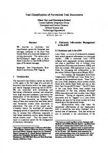
Time Series for “January” Original (Top Left), Non-Periodic Component (Top Right), Periodic Component (Bottom Right)
500 400 300 200 100 0
4000
10000 9000
3500
8000
3000
7000
2500
6000 5000
2000
4000
1500
3000
1000
2000
500
1000
0
0 1
164 327 490 653 816 979 1142 1305 1468 1631 1794 1957
1
161 321 481 641 801 961 1121 1281 1441 1601 1761 1921 2081
1
161 321 481 641 801 961 1121 1281 1441 1601 1761 1921 2081
9000
Time Series for “The” Original (Top Left), Non-Periodic Component (Top Right), Periodic Component (Bottom Right)
8000 7000 6000 5000 4000 3000 2000 1000 0
Figure 1: Effects of applying the temporal periodical algorithm on time series for "January" (top three graphs) and "the" (bottom three graphs) with the original series on the left and the remaining time series components after filtering on the right. Y-axis shows frequency count and X-axis shows the day number (time).
3
left after the periodic component has been filtered out from the original time series. Figure 1 shows an example of the filtering results on timeseries of the words “January” and “the”. The original series is presented together with two series representing the periodic and non-periodic
Temporal Periodicity Analysis
We have created a high-performance system that decomposes time series into two parts: a periodic component that repeats itself in a predictable manner, and a non-periodic component that is 19
components of the original time series. The time series are based on training documents selected at random from the GigaWord English corpus. 10% of all the documents in the corpus were used as training documents, with the rest being available for evaluation and testing. A total of 395,944 time series spanning 9 years were calculated from the GigaWord corpus. The availability of 9 years of data also mitigated the negative effects of using short time series in combination with SARIMA models (as up to 3,287 data points were available for some words, well above the 50 data point minimum recommendation). Figure 2 presents pseudo-code for the time series decomposition algorithm:
names (“Monday”, “Tuesday”, etc.) Note that the frequency counts peak exactly on that particular day of the week. Thus, for example, the word “Monday” is automatically associated with Day 1, and “April” associated with Month 4. The creation of temporal association rules generalises the inferences obtained from the periodic data. Each association rule has the following information: • • •
Word ID Period Type (Week, Month, etc.) Period Number and Score Matrix
The period number and score matrix represent a probability density function that shows the likelihood of a word appearing on a particular period number. Thus, for example, the score matrix for “January” will have a high score for period 1 (and period type set to Monthly). Figure 4 shows some examples of extracted association rules. The probability density function (PDF) scores are shown in Figure 4 as they are stored internally (as multiples of the standard deviation of that time series) and are automatically normalised during the classification process at runtime. The standard deviation of values in the time series is used instead of absolute values in order to reduce the variance between fluctuations in different time series for words that occur frequently (like pronouns) and those that appear relatively less frequently. Rule generalisation is not possible in such a straightforward manner for the non-periodic data. In this paper, the use of non-periodic data to optimise the results of the temporal classification and automatic dating system is not covered. Nonperiodic data may be used to generate specific rules that are associated only with particular dates or date ranges. Non-periodic data can also use information obtained from hapax words and other low-frequency words to generate additional refinement rules. However, there is a danger that relying on rules extracted from non-periodic data will simply reflect the specific characteristics of the corpus used to train the system, rather than the language in general. Ongoing research is being performed into calculating relevance levels for rules extracted from non-periodic data.
1. Find min/max/mean and standard deviation of time series 2. Start with a pre-defined maximum window size (set to 366 days in our present system) 3. While window size bigger than 1 repeat steps a. to d. below: a. Look at current value in time series (starting from first value) b. Do values at positions current, current + window size, current + 2 x window size, etc. vary by less than half a standard deviation? c. If yes, mark current value/window size pair as being possible decomposition match d. Look at next value in time series until the end is reached e. Decrease window size by one 4. Select the minimum number of decomposition matches that cover the entire time series using a greedy algorithm
Figure 2: Time Series Decomposition Algorithm
The time series decomposition algorithm was applied to the 395,944 time series, taking an average of 419ms per series. The algorithm runs in O(n log n) time for a time series of length n. The periodic component of the time series is then analysed to extract temporal association rules between words and different “seasons”, including Day of Week, Week Number, Month Number, Quarter, and Year. The procedure of determining if a word, for example, is predominantly peaking on a weekly basis, is to apply a sliding window of size 7 (in the case of weekly periods) and determining if the periodic time series always spikes within this window. Figure 3 shows the frequency distribution of the periodic time series component of the days of week
4
Temporal Classification and Automatic Dating
The periodic temporal association rules are utilised to guess automatically the creation date of 20
documents. Documents are input into the system and the probability density functions for each word are weighted and added up. Each PDF is weighted according to the inverse document frequency (idf) of each associated word. Periods that obtain high score are then ranked for each type of period and two guesses per period type are obtained for each document. Ten guesses in total are thus obtained for Day of Week, Week Number, Month Number, Quarter, and Year (5 period types x 2 guesses each). 0 1 2 3 4 5 6 Av St
Su
M
22660
10540
T 7557
W 772
Th 2130
F 3264
12461
37522
10335
6599
1649
3222
3414
3394
18289
38320
9352
7300
2543
2261
2668
4119
18120
36933
10427
5762
2147
2052
2602
3910
17492
36094
9098
5667
5742
1889
2481
2568
17002
32597
7849
7994
7072
1924
1428
3050
14087
21468
8138
11719
11806
10734
11093
10081
7782
7357
12711
12974
12933
12308
10746
6930
document. The system has been integrated with a fine-grained temporal analysis system based on TimeML, with promising results, especially when processing documents obtained from the Internet.
5
The system was trained using 67,000 news items selected at random from the GigaWord corpus. The evaluation took place on 678,924 news items extracted from items marked as being of type “story” or “multi” in the GigaWord corpus. Table 1 presents a summary of the evaluation results. Processing took around 2.33ms per item. The actual date was extracted from each news item in the GigaWord corpus and the day of week (DOW), week number and quarter calculated from the actual date. This information was then used to evaluate the system performance automatically. The average error for each type of classifier was also calculated automatically. For a result to be considered as correct, the system had to have the predicted value ranked in the first position equal to the actual value (of the type of period).
S 11672
Figure 3: Days of Week Temporal Frequency Distribution for extracted Periodic Component displayed in a Weekly Period Type format January Week 1 Score 1.48
2 2.20
Month 1 Quarter
Score 2.95 1 Score 1.50
Christmas Week 2 Score 1.32 Week 47 Score 1.32
5 0.73 49 2.20
36 1.60 50 2.52
42 0.83 51 2.13
44 1.32 52 1.16
Month Score
9 0.75
10 1.63
11 1.73
12 1.98
4
Score 1.07
1 1.10
Quarter
3 3.60
4 3.43
Type
5 3.52
DOW Week Month Quarter Year
Correct 218,899 (32.24%) 24,660 (3.53%) 122,777 (18.08%) 337,384 (49.69%) 596,009 (87.78%)
Incorrect 460,025 (67.75%) 654,264 (96.36%) 556,147 (81.91%) 341,540 (50.30%) 82,915 (12.21%)
Avg. Error 1.89 days 14.37 wks 2.57 mths 1.48 qts 1.74 yrs
Table 1: Evaluation Results Summary
The system results show that reasonable accurate dates can be guessed at the quarterly and yearly levels. The weekly classifier had the worst performance of all classifiers, likely as a result of weak association between periodical word frequencies and week numbers. Logical/sanity checks can be performed on ambiguous results. For example, consider a document written on 4 January 2006 and that the periodical classifiers give the following results for this particular document: • DOW = Wednesday • Week = 52 • Month = January
Figure 4: Temporal Classification Rules for Periodic Components of "January" and "Christmas"
4.1
Evaluation, Results and Conclusion
TimeML Output
The system can output TimeML compliant markup tags using TIMEX that can be used by other TimeML compliant applications especially during temporal normalization processes. If the base anchor reference date for a document is unknown, and a document contains relative temporal references exclusively, our system output can provide a baseline date that can be used to normalize all the relative dates mentioned in the 21
• Quarter = 1 • Year = 2006 These results are typical of the system, as particular classifiers sometimes get the period incorrect. In this example, the weekly classifier incorrectly classified the document as pertaining to week 52 (at the end of the year) instead of the beginning of the year. The system will use the facts that the monthly and quarterly classifiers agree together with the fact that week 1 follows week 52 if seen as a continuous cycle of weeks to correctly classify the document as being created on a Wednesday in January 2006. The capability to automatically date texts and documents solely from its contents (without any additional external clues or hints) is undoubtedly useful in various contexts, such as the forensic analysis of undated instant messages or emails (where the Day of Week classifier can be used to create partial orderings), and in authorship identification studies (where the Year classifier can be used to check that the text pertains to an acceptable range of years). The temporal classification and analysis system presented in this paper can handle any IndoEuropean language in its present form. Further work is being carried out to extend the system to Chinese and Arabic. Evaluations will be carried out on the GigaWord Chinese and GigaWord Arabic corpora for consistency. Current research is aiming at improving the accuracy of the classifier by using the non-periodic components and integrating a combined classification method with other systems.
Ferro, L. Gerber, L. Mani, I. Sundheim, B. Wilson, G. 2004. TIDES Standard for the Annotation of Temporal Expressions. The MITRE Corporation. Filatova, E. Hovy, E. 2001. Assigning time-stamps to event-clauses. Proc. EACL 2001, Toulouse. Fung, G. 2003. The Disputed Federalist Papers: SVM Feature Selection via Concave Minimization. New York City, ACM Press. Gaizauskas, R. Setzer, A. 2002. Annotation Standards for Temporal Information in NL. LREC 2002. Janacek, G. 2001. Practical Time Series. Oxford U.P. Kiritchenko, S. Matwin, S. Abu-Hakima, S. 2004. Email Classification with Temporal Features. Proc. IIPWM 2004, Zakopane, Poland. Springer Verlag Advances in Soft Computing, pp. 523-534. Linguistic Data Consortium (LDC). 2003. English Gigaword Corpus. David Graff, ed. LDC2003T05. Mani, I. Wilson, G. 2000. Robust temporal processing of news. Proc. ACL 2000, Hong Kong. Mani, I. Schiffman, B. Zhang, J. 2003. Inferring temporal ordering of events in news. Proc. HLTNAACL 2003, Edmonton, Canada. Moldovan, D. Clark, C. Harabagiu, S. 2005. Temporal Context Representation and Reasoning. IJCAI2005, pp. 1099-1104. Mosteller, F. Wallace, D. 1964. Inference and Disputed Authorship: Federalist. Addison-Wesley. Prager, J. Chu-Carroll, J. Brown, E. Czuba, C. 2003. Question Answering using predictive annotation. In Advances in Question Answering, Hong Kong. Pustejovsky, J. Castano, R. Ingria, R. Sauri, R. Gaizauskas, R. Setzer, A. Katz, G. 2003. TimeML: Robust Specification of event and temporal expressions in text. IWCS-5.
References Aramburu, M. Berlanga, R. 1998. A Retrieval Language for Historical Documents. Springer Verlag LNCS, 1460, pp. 216-225.
Pustejovsky, J. Sauri, R. Castano, J. Radev, D. Gaizauskas, R. Setzer, A. Sundheim, B. Katz, G. 2004. “Representing Temporal and Event Knowledge for QA Systems”. New Directions in QA, MIT Press.
Berlanga, R. Perez, J. Aramburu, M. Llido, D. 2001. Techniques and Tools for the Temporal Analysis of Retrieved Information. Springer Verlag LNCS, 2113, pp. 72-81.
Schilder, F. Habel, C. 2003. Temporal Information Extraction for Temporal QA. AAAI Spring Symp., Stanford, CA. pp. 35-44.
Boguraev, B. Ando, R.K. 2005. TimeML-Compliant Text Analysis for Temporal Reasoning. IJCAI2005, pp. 997-1003.
Silverstein, C. Brin, S. Motwani, R. 1997. Beyond Market Baskets: Generalizing Association Rules to Dependence Rules. Data Mining and Knowledge Discovery.
Box, G. Jenkins, G. 1976. Time Series Analysis: Forecasting and Control, Holden-Day.
Sundheim, B. Gerber, L. Ferro, L. Mani, I. Wilson, G. 2004. Time Expression Recognition and Normalization (TERN). MITRE, Northrop Grumman, SPAWAR. http://timex2.mitre.org.
Brockwell, P.J. Fienberg, S. Davis, R. 1991. Time Series: Theory and Methods. Springer-Verlag. Chatfield, C. 2003. The Analysis of Time Series. CRC Press.
Yarowsky, D. 1994. Decision Lists For Lexical Ambiguity Resolution: Application to Accent Restoration in Spanish and French. ACL 1994.
22