1 Introduction. Shrinking the semiconductor devices requires accurate investigations by means of simulation. Numerical modelling was first suggested by ...
SIMULATION OF SEMICONDUCTOR DEVICES AND PROCESSES Vol. 4 Edited by W. Fichtner, D. Aemmer - Zurich (Switzerland) September 12-14,1991
- Hartung-Gorre
Automatic Device Characterization Institute
P e t e r Verhas and Siegfried Selberherr for Microelectronics, Technical University of Vienna,
Austria
Abstract An automatic device characterization tool was developed. This tool chooses bias points automatically adapting itself to nonlinearities for simulation of semiconductor devices and builds up a table for interpolation. This table can later be used for fast calculation of device behavior instead of invoking the simulator during device parameter extraction.
1
Introduction
Shrinking the semiconductor devices requires accurate investigations by means of simulation. Numerical modelling was first suggested by Gummel [1] in 1964. Since t h a t time numerical semiconductor device simulators have become well-known and widely used. Today semiconductor device development without simulation is unimaginable. The daily work of an engineer using simulators is to produce input for the simulators, run t h e m and read and interpret the results. This work contains a lot of tedious actions and significant research is done nowadays to automatize it as much as possible. One approach is to build device characterization tools t h a t calculate the characteristics of a device using simulators over a given region of input parameters by automatically adapting itself to the nonlinearities and building up a table. This table is used later for interpolation. It can be used to derive basic device parameters or applied in circuit simulators [2]. Such a tool was developed using a two-dimensional algorithm. It has been applied for M O S F E T simulation using the simulator MINIMOS [3]. In this paper a procedure is detailed which creates the interpolation table automatically. First a one-dimensional algorithm is discussed in section 3. This algorithm is extended for two dimensions in section 4 and experiments were m a d e using this algorithm using the MOS simulator MINIMOS.
2
Requirements for automatic table generation
The requirements can be grouped into two categories: the conditions t h a t automatic device characterization needs, and what it should fulfill. The automatic table generation needs a simulation environment where it is possible to start a simulation automatically for several bias points. This requirement is fulfilled by the VISTA system [4]. The requirements for the a u t o m a t i c table generator are the following: • The bias points, for which the simulator is started, should be calculated automatically. • The points t h a t are simulated should cover the bias domain dense enough to enable accurate interpolation.
400
• The points should be more dense at nonlinear regions and sparse at linear regions. This way the interpolation error does not depend on the location and is lower everywhere than a given limit. • The storage of the result of the simulations should be compact. • The structure of the points should be suited for a fast interpolation tool. • The different bias points should be simulated in an order that the result of previous calculations can be used for the initial solution estimation in the next simulation step. • Bias points which are computationally cheap (low voltages) should be calculated first and initial solution extrapolation should be applied for the higher voltages. • Parameters should easily be estimated
3
One—dimensional mapping
The one-dimensional algorithm is similar to the algorithm published in [5] with some extensions. A function / : R >-> R can be defined with a finite number of points (xi, f(%i)), (x2, f(x2)), • • •, (z n , /(«„)) within an interval. The slope of the function in [a:;, a;»+i] is /(s»+i) ~ / ( * 0 s.
-
m
.
(XJ
The nonlinearity of the function at the point xi is defined as di~
S{ - S i _ i .
(2)
The definition of the resolution is a = maxdj-.
(3)
»=2
Using this definition the resolution is strongly linked with the error of the interpolation based on the points {xu / (aii)), (x2, f(x2)),..., (xn, f(xn)). To characterize a device with one free parameter (like drain voltage) one should specify the range of the characterization (i.e. minimal and maximal value for the parameter), the required resolution of the mapping and an estimated value for the average size of an interval A. The algorithm: 1. Calculate the function at the points XQ — xmin, x\ = xmin + A and x2 = xmin + 2A. 2. Set i = 1. 3. If di > a then the last interval was too long, refine it calculating a new point inside. 4. Estimate a new value for A according to the nonlinearity of the function at the point X{ using the expression Cx Aneuj — T ' "old-
di
5. Set i = i + 1 and a;,- = ai;_i + A. 6. If £,- < xmax
calculate f(x{) and go to 3.
V.4J
401
Figure 1: Definition of nonlinearity During experiments it turned out that some refinement of the algorithm above is required. These refinements do not effect the base of the algorithm and the adaptation of the step size due to nonlinearity. To avoid infinite shortening of A due to numerical inaccuracies of the simulator we denned a minimal value Xmin- A function being almost linear near the point xmin causes the problem that the calculated value of A after the third step is too high. We introduce Xmax that stands for the maximal allowed value of A. As the above algorithm does not calculate the f(xmax), the interpolation is inaccurate for points being larger than the last calculated. Therefore the value f(xmax) is always calculated, and if xmax - X{ < Xmin then £; is set to xmax at point 6. The program does not use the value of A as input but the approximated number of the required points N. The calculation of A is defined by the expression K
(5) N The value of K is an arbitrary positive value in the order 0(1). It is to note that for functions which are almost linear around the point xmin a value of K > 1.0 fits, and for functions which are strongly nonlinear at the start K < 1.0 is better. The algorithm is very sensitive to the value of a and specifying a too low value causes too many points to be calculated. As an extreme case [(xmax — a; mt „)/A m i n ] + 1 points will be calculated for a = 0.0. Fortunately we do not use the one dimensional algorithm alone and the two-dimensional case gives the possibility to eliminate this weakness.
4
Two-dimensional mapping
To map a function f(x,y) on the domain xmin < x < xmax and ymin < y < Vmax using the one-dimensional algorithm one can define some g: [zmin, zmax] h-> R2 functions and apply the algorithm for the composite function h(z) = f(g(z)). The function g(z) = (x • g(z),y- g(z)) defines a curve on the domain. The simplest way is to choose functions of the form g(z) = (Axz + Bx,Ayz where Ax,Bx,Ay,By
+ By)
(6)
are constant values and \xmin
•£>x)Ay — \ymin
"yj-^-3
(7)
402
holds. In this case the curves defined by g(z) are straight lines including the point (£„,,„, t/ m ; n ). Without loss of generality we can assume that for any zi,z2 € (zmin, zmax) the expression (zi — Z2)2 = \\g(zi) — ^(22)|| is true. This scaling is useful when the two axes have the same dimension (voltage in our experiments). In other cases one can set the values of zm,-n and zmax to 0 and 1 respectively. We say that two such lines g\ and g2 are neighbour lines on a subset of the set of this type of lines if there is no line g$ in the subset for which AxiAX3 < AyiAy3 and Ax^Ax2 < Ay3Ay2 holds assuming Ax\Axi < Ay\Ay2. {Avi means the Au coefficient for the function (3X.
(11)
Let gi{z)
= (Axix + Bxi, Ayiy -V Byi)
(12)
where
r* = ^(iv, + r„fc)
(13)
and T and v stand for all possible combinations of A, B and x, y. If there are no such lines then stop. Set z m j n so that \\gi{zmin
~ 9k(Zmin)\\
= /3A
(14)
and set zmax so that Zmax = max{z: x • gi(z) < xmax
A y-gi(z)
< ymax}-
(15)
Set ai
= -(ai + ak).
(16)
Map the line gi using the one-dimensional algorithm, and after mapping calculate a value for cti that would have been the best for the mapping. 4. Set i = i + 1 and go to 3.
403
'max^
'mm min
D Calculated Bias Points
max
Figure 2: Geometry of calculated points One can see that following the instructions the geometrical place of the lines is determined by the values of xmin,xmax,ymin,ymax,X and /3. Therefore the total length L of the lines can be calculated, and a function L = 7 (A) (17) can describe the relationship. One can also see that 7(A) is monotonically decreasing. On the other hand if the total length of the lines L and the number of the expected points n are known, the average step size I, can be calculated. 7(A) (18) N Assuming that the distance between neighbouring points should be approximately the same on one line and between neighbouring lines we can say that the value of A and ls should be the same. Putting equations (17) and (18) together we get an equation /, = L/N
N
(19)
which can be solved iteratively. The value of /3 in equation (14) is an arbitrary constant value around 2.0. In steps 2 and 3 we calculate a values for lines that are already mapped. In this action we know the length of the line and the expected average interval length l3. These two values define the expected number of the points on the given line, n. If we have less than n points, we just take the resolution of the curve. If the number of the calculated points k is larger than n, the used a value was too small. In this case we calculate the resolution of the line according to equation (3) neglecting those k - n points for which the value d{ is the highest. This resolution value gives an approximation for a that would have been good for the mapping. We use these values in equation (16). The only exception is the calculation of 03 that should not follow this equation because gi and g2 are orthogonal.
404
5
Interpolation
The interpolation in one-dimension can be done using arbitrary scheme. Using the a-priori knowledge that the function is monotonic one can for instance use monotonic spline interpolation as it is suggested in [2]. The 2D interpolation is based on some one-dimensional interpolation. To interpolate a value for the point (x,y) we should examine the lines gx(z) = {x,z)
(20)
gy(z) = (z,y).
(21)
and Unless x = xmin the set Sx = gx U g\ U . . . U gn has only finit number of points. Similarly if y 7^ ymin the set Sy = gx U g\ U -.. U gn is finite. Choose the line gv if \SV\ > |5"n|. Calculate the value of the function / at the points Sv using one-dimensional interpolations along all lines gi for which gu U gi ^ 0 and using the line gv interpolate a value for f(x,y) based on the points S„. This interpolation produces a smooth surface over all the domain except for the region where \SX\ = \Sy\. In this region the interpolated function has discontinuities because the direction of the interpolation changes. However it is to note that these discontinuities are within the range of the error of the interpolation. To remove these we build up an equidistant dense mesh over the domain and later we use this mesh to interpolate. For each point of the mesh we use the interpolation described above and when the mesh is ready we apply a 2D low pass filtering to increase smoothness and remove discontinuities [6].
6
Results
As a typical example we have applied the algorithm to simulations of strong inversion characteristics of an N-channel MOSFET using MINIMOS. The boundary values were J7z)m,n = 1.0F, Uomax = 8.OF, UGmin = 1.0V, UGmax = 6.OF. This boundary covers the normal operating region of a typical switching MOSFET for open state, but does not include the subthreshold region. To calculate the points of this region is enough for most of the parameter extraction tools. We have set the value of the expected points N = 200. The algorithm produces 187 points. Extending the boundary to Uomax = 14.OF including the breakdown region the algorithm produces 195 points. As shown in Figure 3, the points are more dense at low drain voltages where the function ID{UD,UG) is nonlinear, sparse at the saturation region and dense at the breakdown region where the function is strongly nonlinear. One can see very dense points in the breakdown region. This was generated because the value Am;n was set too low and numerical inaccuracies forced the algorithm to decrease X down to A m i n . Our experiments show that the value of AT in equation (5) should be around 1.5 for simulation of MOS transistor strong inversion characteristics with Up or UG as parameter and xmin ss UthIn the example that is shown in Figure 3 the value K — 1.61 was used. To check the error of the interpolation we calculated a 0.2V equidistant mesh over the larger area using the simulator and compared it to the interpolated values. The relative error of the interpolation is below 2% everywhere on both of the domains. This error is small enough for any practical purpose and the simulation can be replaced by table interpolation.
405
Figure 3: MINIMOS simulation, 195 points
7
Conclusion
In this paper we have described a method to characterize devices automatically. The characterization covers a two-dimensional domain and so the algorithms described in [5] are extended from "Curve-Tracer" into "Plane-Tracer" mode. The algorithms support initial solution estimation for the device simulator and this improves the simulator convergence. The method produces a data structure that can be used for interpolation of scalar or distributed physical quantities with good accuracy. The number of the required points is low taking into account that the simulation time can radically be reduced by the initial solution estimation. The algorithm was constructed taking into account the possibility of further multi-dimensional expansion.
Acknowledgements This project is supported by the research laboratories of: AUSTRIAN INDUSTRIES - AMS Int. at Unterpremstatten, Austria; DIGITAL EQUIPMENT Corp. at Hudson, USA; SIEMENS Corp. at Munich, FRG; and SONY Corp. at Atsugi, Japan.
References [l] H.K. Gummel, A self-consistent iterative scheme for one-dimensional steady state transistor calculations., IEEE Trans. Electron Devices, ED-11, pp. 455-465, 1964 [2] Takeshi Shima, Hisashi Yamada, and Ryo Luong Mo Dang, Table look-up mosfet modeling system using a 2-d device simulator and monotonic piecewise cubic interpolation., IEEE Trans, on Computer-Aided Design of Integrated Circuits and Systems, CAD-2, pp. 121126, 1983
406
[3] S. Selberherr, Three dimensional device modeling with MINIMOS 5, In Proceedings VLSI Process/Device Modeling Workshop, pp. 40—41, 1989 [4] F. Fasching et at, An Integrated Technology CAD Environment, Proc. Int. Symp. on VLSI Technology, Systems and Applications, Taipei, Taiwan, 1991 [5] Robert W. Dutton and Zhiping Yu, Algorithms for curve-tracer mode in simulation of devices with highly nonlinear characteristics, In Proceedings VLSI Process/Device Modeling Workshop, pp. 24-27, 1990 [6] William H. Press, Brian P. Flannery, Saul A. Teukolsky, and William T. Vetterling, Numerical Recipes, Cambridge University Press, 1st edition, 1988