Automatic Differentiation for GPU-Accelerated 2D/3D. Registration. Markus Grabner, Thomas Pock, Tobias Gross, and Bernhard Kainz. Institute for Computer ...
Automatic Differentiation for GPU-Accelerated 2D/3D Registration Markus Grabner, Thomas Pock, Tobias Gross, and Bernhard Kainz Institute for Computer Graphics and Vision, Graz University of Technology, Inffeldgasse 16a/II, 8010 Graz, Austria
Summary. A common task in medical image analysis is the alignment of data from different sources, e.g., X-ray images and computed tomography (CT) data. Such a task is generally known as registration. We demonstrate the applicability of automatic differentiation (AD) techniques to a class of 2D/3D registration problems which are highly computationally intensive and can therefore greatly benefit from a parallel implementation on recent graphics processing units (GPUs). However, being designed for graphics applications, GPUs have some restrictions which conflict with requirements for reverse mode AD, in particular for taping and TBR analysis. We discuss design and implementation issues in the presence of such restrictions on the target platform and present a method which can register a CT volume data set (512 × 512 × 288 voxels) with three X-ray images (512 × 512 pixels each) in 20 seconds on a GeForce 8800GTX graphics card. Key words: Optimization, medical image analysis, 2D/3D registration, GPU
1 Introduction Accurate location information about the patient is essential for a variety of medical procedures such as computer-aided therapy planning and intraoperative navigation. Such applications typically involve image and volume data of the patient recorded with different devices and/or at different points in time. In order to use these data for measurement purposes, a common coordinate system must be established, and the relative orientation of all involved coordinate systems with respect to the common one must be computed. This process is referred to as registration. Variational methods [5] are among the most successful methods to solve a number of computer vision problems (including registration). Basically, variational methods aim to minimize an energy functional which is designed to appropriately describe the behavior of a certain model. The variational approach provides therefore a way to implement non-supervised processes by just looking for the minimizer of the energy functional. Minimizing these energies is usually performed by calculating the solution of the EulerLagrange equations for the energy functional. For quite involved models, such as the energy functional we use in our 2D/3D registration task, their analytical differentiation is not a trivial task and is moreover error prone. Therefore many people bypass this issue by computing the
2
Markus Grabner, Thomas Pock, Tobias Gross, and Bernhard Kainz
derivatives by means of a numerical approximation. This is clearly not optimal and can lead to inaccurate results. In [26] automatic differentiation methods have been studied in the context of computer vision problems (denoising, segmentation, registration). The basic idea is to discretize the energy functional and then apply automatic differentiation techniques to compute the exact derivatives of the algorithmic representation of the energy functional. Recently, graphics processing units (GPUs) have become increasingly flexible and can today be used for a broad range of applications, including computer vision applications. In [25] it has been shown that GPUs are particularly suitable to compute variational methods. Speedups of several orders of magnitude can be achieved. In this paper we propose to take advantage of both automatic differentiation and the immense computational power of GPUs. Due to the limited computational flexibility of GPUs, standard automatic differentiation techniques can not be applied. In this paper we therefore study options of how to adapt automatic differentiation methods for GPUs. We demonstrate this by means of medical 2D/3D registration. The remainder of this article is organized as follows: in Sect. 2 we give a brief literature review about automatic differentiation and medical registration. We give then technical details about the 2D/3D registration task in Sect. 3, and the limitations of currently available GPU technologies and our proposed workaround are discussed in Sect. 4. We demonstrate the usefulness of our approach in Sect. 5 by means of experimental results of synthetic and real data. Finally, in Sect. 6 we give some conclusions and suggest possible directions for future investigation.
2 Related Work Automatic differentiation is a mathematical concept whose relevance to natural sciences has steadily been increasing in the last twenty years. Since differentiating algorithms is, in principle, tantamount to applying the chain rule of differential calculus [9], the theoretic fundamentals of automatic differentiation are long-established. However, only recent progress in the field of computer science places us in a position to widely exploit its capabilities [10]. Roughly speaking, there are two elementary approaches to accomplishing this rather challenging task, namely source transformation and operator overloading. Prominent examples of AD tools performing source transformation include Automatic Differentiation of Fortran (ADIFOR) [3], Transformation of Algorithms in Fortran (TAF) [7], and Tapenade [13]. The bestknown AD tool implementing the operator overloading approach is Automatic Differentiation by Overloading in C++ (ADOL-C) [11]. There is a vast body of literature on medical image registration, a good overview is given by Maintz and Viergever [19]. Many researchers realized the potential of graphics hardware for numerical computations. GPU-based techniques have been used to create the digitally reconstructed radiograph (DRR), which is a simulated X-ray image computed from the patient’s CT data. Early approaches are based on texture slicing [18], while more recent techniques make use of 3D texture hardware [8]. The GPU has also been used to compute the similarity between the DRR and X-ray images of the patient [17]. K¨ohn et al. presented a method to perform 2D/2D and 3D/3D registration on the GPU using a symbolically calculated gradient [15]. However, they do not deal with the 2D/3D case (i.e., no DRR is involved in their method), and they manually compute the derivatives, which restricts their approach to very simple similarity measures such as the sum-of-squares difference (SSD) metric. A highly parallel approach to the optimization problem has been
AD for 2D/3D Registration on the GPU
3
( t x , t y , tz , φ, θ , ψ )T (a) C T scanner (computed tomography)
(b) C T volume (set of slices)
(e) mobile X -ray device (C-arm)
(c) tr ansformation par ameters
(f) X- ray image
(d) digitally reconstructed radiograph
(g) GPU-based 2D/3D-registration
Fig. 1. Schematic workflow of 2D/3D registration. Before the intervention, a CT scanner (a) is used to obtain a volumetric data set (b) of the patient. With an initial estimate for the transformation parameters (c), which we seek to optimize, a DRR (d) is created from the volume data. During the intervention, a C-arm (e) is used to obtain X-ray images (f) of the patient. The registration procedure (g) compares the DRR and X-ray image and updates the transformation parameters until the DRR is optimally aligned with the X-ray image (i.e., our distance measure is minimized). We use three DRR/X-ray image pairs for better accuracy (only one is shown here). proposed by Wein et al. [27]. They perform a best neighbor search in any of the six degrees of freedom, i.e., they require 12 volume traversals per iteration, where each traversal is done on a separate processor.
3 Review of 2D/3D Registration The 2D/3D rigid registration task as outlined in Fig. 1 can be formulated as an optimization problem, where we try to find the parameter vector xopt ∈ R6 of a rigid transformation in 3D such that the n projections Ii (x) of our CT volume (i.e., the DRRs) are optimally aligned with a set of n X-ray images Ji , i = 1 . . . n. Formally, we try to solve xopt = argmin E(x), x
E(x) = ∑ D(Ii (x), Ji )
(1)
i
where E is our cost function, and D(Ii (x), Ji ) computes the non-negative distance measure between two images, which is zero for a pair of perfectly aligned images. Note that the Xray images Ji do not depend on the parameter vector x, but each X-ray image has an exterior camera orientation [12] associated with it (describing the recording geometry), which must be used to compute the corresponding DRR Ii (x). The computation of the camera orientation is out of the scope of this paper. In the following, we only deal with a single pair of images and leave the summation in Eq. (1) as a final (implicit) processing step.
3.1 Digitally Reconstructed Radiograph To adequately simulate the process of X-ray image acquisition, we have to understand what the image intensities of the radiograph arise from. The X-ray intensity I reaching the detector
4
Markus Grabner, Thomas Pock, Tobias Gross, and Bernhard Kainz
Algorithm 1 The DRR rendering algorithm. All transformations are given as 4 × 4 matrices in homogeneous coordinates, where T and R are translation and rotation, respectively, C describes the center of rotation, and H is the window-to-object coordinates transformation. d is the sampling distance in window coordinates. Ω is the set of pixels (u, v) which are covered by the projection of the volume, and Ω(u,v) is the set of sampling positions along the ray through pixel (u, v) which intersect the volume. µ(p) is the volume sample at point p. Require: C, R, T, H ∈ M4 (R) ; d ∈ R+ 1: for all (u, v) ∈ Ω do (0) 2: pwin = (u, v, d/2, 1)T 3: dwin = (0, 0, d, 1)T (0) (0) 4: pobj = CR−1 T−1 C−1 Hpwin 5: 6: 7:
{ray start position in window coordinates} {ray step vector in window coordinates} {ray start position in object coordinates}
dobj = CR−1 T−1 C−1 Hdwin I(u, v) = 0 for all t ∈ Ω(u,v) do
{ray step vector in object coordinates}
(0)
8: I(u, v) = I(u, v) + µ(pobj + tdobj ) 9: end for 10: end for
{take volume sample and update intensity}
at a pixel (u, v) ∈ Ω in image space can be expressed using the following physically-based model [27]: µ Z ¶ Z Emax Iphys (u, v) = I0 (E) exp − µ(x, y, z, E)dr dE, (2) 0
r(u,v)
where I0 (E) denotes the incident X-ray energy spectrum, r(u, v) a ray from the X-ray source to the image point (u, v), and µ(x, y, z, E) the energy dependent attenuation at a point (x, y, z) in space. The second integral represents the attenuation of an incident energy I0 (E) along the ray r(u, v). The integral over E incorporates the energy spectrum of X-ray cameras. The above expression can be simplified in several ways [27]. First, the X-ray source is mostly modeled to be monochromatic and the attenuation to act upon an effective energy Eeff . Second, due to the fact that X-ray devices usually provide the logarithm of the measured Xray intensities, we can further simplify Eq. (2) by taking its logarithm. Finally, when using more elaborate similarity measures which are invariant with respect to constant additions and multiplications [19], we can omit constant terms and obtain the following pixel intensities for our DRR image: Z I(u, v) = r(u,v)
µ(x, y, z, Eeff )dr
(3)
The pseudo code of the DRR rendering algorithm under the parameter vector x = (tx ,ty ,tz , φ , θ , ψ)T is given in Alg. 1. The rigid body transformation we seek to optimize in Fig. 1(c) consists of a translation t = (tx ,ty ,tz )T and a rotation R = Rψ Rθ Rφ given in terms of three Euler angles φ , θ , and ψ, where cos φ sin φ 0 cos θ 0 − sin θ 1 0 0 Rφ = − sin φ cos φ 0 , Rθ = 0 1 0 , Rψ = 0 cos ψ sin ψ 0 0 1 sin θ 0 cos θ 0 − sin ψ cos ψ
AD for 2D/3D Registration on the GPU
5
3.2 Similarity Measure We investigate the normalized cross correlation, which verifies the existence of an affine relationship between the intensities in the images. It provides information about the extent and the sign by which two random variables (I and J in our case) are linearly related: ¡ ¢¡ ¢ ∑(u,v)∈Ω I(u, v) − I J(u, v) − J q (4) NCC (I, J) = q ¢2 ¢2 ¡ ¡ ∑(u,v)∈Ω I(u, v) − I ∑(u,v)∈Ω J(u, v) − J Optimal alignment between the DRR image I and the X-ray image J is achieved for NCC(I, J) = −1 since we use Eq. (3) for DRR computation, but the actual X-ray image acquisition is governed by Eq. (2). Our distance measure from Eq. (1) is therefore simply D(Ii (x), Ji ) = NCC(Ii (x), Ji ) + 1.
3.3 Iterative Solution We chose the L-BFGS-B algorithm [28] to accomplish the optimization task because it is easy to use, does not depend on the computation of second order derivatives, and does not require any knowledge about the structure of the cost function. Moreover, it is possible to set explicit bounds on the subset of the parameter space to use for finding the optimum.
4 Automatic Differentiation for a hybrid CPU/GPU Setup In this section we address several issues that must be considered when applying AD techniques to generate code that will be executed in a hybrid CPU/GPU setup for maximum performance. Before we do so, however, we give a brief review of currently available computing technologies for GPUs and compare their strengths and weaknesses in the given context.
4.1 GPU Computing Technologies The Cg language developed by NVidia [20] allows the replacement of typical computations performed in the graphics pipeline by customized operations written in a C-like programming language. It makes use of the stream programming model, i.e., it is not possible to communicate with other instances of the program running at the same time or to store intermediate information for later use by subsequent invocations. Moreover, local memory is limited to a few hundred bytes, and there is no support for indirect addressing. This makes it impossible to use arrays with dynamic indices, stacks, and similar data structures. On the other hand, this computation scheme (which is free of data inter-dependences) allows for very efficient parallel execution of many data elements. Furthermore, Cg has full access to all features of the graphics hardware, including the texture addressing and interpolation units for access to 3D texture data. Similar functionality as in Cg is available in the OpenGL Shading Language (GLSL), which is not separately discussed here. The Compute Unified Device Architecture (CUDA) by NVidia [23] is specifically designed for the use of graphics hardware for general-purpose numeric applications. As such, it also allows arbitrary read and write access to GPU memory and therefore seems to be the ideal candidate for our implementation. However, the current version 1.1 of CUDA lacks native support for 3D textures, so access to CT data would have to be rewritten as global memory access, which neither supports interpolation nor caching. Such a workaround would impose severe performance penalties, we therefore decided to use Cg since the intermediate storage problem can more easily be overcome as we will see in the remainder of this section.
6
Markus Grabner, Thomas Pock, Tobias Gross, and Bernhard Kainz
4.2 Computing Resources In order to properly execute both the original algorithm and its derivative, we must determine which hardware component is best suited for each section of the algorithm. The following components are available to us: • • •
the host’s CPU(s), the GPU’s rasterizer, and the GPU’s shader processors.
The CPU’s involvement in the numeric computations is marginal (its main task is to control the workflow), we therefore did not consider the use of more than one CPU. Due to the stream programming model in Cg, the output of the shader program is restricted to a fixed (and small) number of values, sufficient however to write a single pixel (and the corresponding adjoint variables) of the DRR. Therefore looping over all pixels in the image (equivalent to (u, v) ∈ Ω in Alg. 1) is left to the rasterizer. The core of the computation is the traversal of the individual rays through the volume (equivalent to t ∈ Ω(u,v) in Alg. 1). Since the CT volume is constant, data can be read from (read-only) texture memory, and the innermost loop can be executed by the shader processors. This procedure has good cache coherence since a bundle of rays through neighboring pixels will likely hit adjacent voxels, too, if the geometric resolutions of image and volume data and the sampling distance are chosen appropriately. The loops in the similarity measurement code, corresponding to the sums in Eq. (4), are more difficult to handle, although the domain (u, v) ∈ Ω is the same as above. The reason is the data-interdependence between successive invocations of the loop body, which must not proceed before the previous run has updated the sum variables. We therefore employ a reduction technique [24], where the texture is repeatedly downsampled by a factor of two (n times for an image 2n × 2n pixels large) until we end up with a single pixel representing the desired value. The optimizer is executed entirely on the CPU and invokes the function evaluation and gradient computation as needed for the L-BFGS-B algorithm (Sect. 3.3).
4.3 Gradient Computation We need to compute the gradient of the (scalar-valued) cost function (Eq. 1) with respect to the transformation parameter vector x ∈ R6 . This can be done either by invoking the algorithm’s forward mode derivative six times or by a single pass of the algorithm’s reverse mode derivative. Every pass of the original and the derived algorithm (both in forward and reverse mode) requires access to all voxels visible under the current transformation parameters at least once (or even several times in case of texture cache misses). Since global memory traffic is the main bottleneck of many GPU-based algorithms, we choose reverse mode AD for our purposes to reduce the number of read operations from texture memory. Reverse mode AD is known to be more difficult to implement than forward mode AD. Due to the above-mentioned memory limitations it is generally not possible to use techniques like taping [21] and TBR analysis [14, 22] to produce adjoint code in Cg. However, since the inner loop in Alg. 1 is simply a sum, we do not need to store intermediate values in the derivative code (i.e., the “TBR set” of our program is empty), hence a Cg implementation is feasible. An additional benefit of the analytically computed gradient is its better numerical behaviour. When computing a numerical approximation of the gradient (e.g., based on central
AD for 2D/3D Registration on the GPU
7
(e)
(a)
(b)
(c)
(d)
(f)
Fig. 2. A simple object with density distribution µ(x, y, z) = 1 − max(|x|, |y|, |z|), x, y, z ∈ [−1, 1], is translated to the left (∆ x < 0) in (a), and the per-pixel contributions to the component of the parameter vector gradient ∇E corresponding to translation in x-direction are visualized in (b), where gray is zero, darker is negative (not present in the image), and brighter is positive. The histogram (e) of the gradient image (b) shows only positive entries (center is zero), indicating an overall positive value of the gradient in x-direction to compensate for the initial translation. In a similar way, the object is rotated (∆ ϕ > 0) in (c), and the gradient contributions with respect to rotation around the z-axis are shown in (d). Its histogram (f) shows a prevalence of negative values, indicating an overall negative rotation gradient around the z-axis to compensate for the initial rotation. All other histograms are symmetric (not shown here), indicating a value of zero for the respective gradient components. differences), one has to carefully find a proper tradeoff between truncation error and cancellation error [4]. This is particularly true with our hardware and software platform (NVidia graphics cards and Cg), where the maximum available precision is 32 bit IEEE floating point.
4.4 Automatic Differentiation Issues The operator overloading technique [6] for generating the algorithm’s derivative can not be used in our case since it requires the target compiler to understand C++ syntax and semantics. However, both Cg and CUDA only support the C language (plus a few extensions not relevant here) in their current versions. Moreover, in order to apply reverse mode AD with operator overloading, the sequence of operations actually performed when executing the given algorithm must be recorded on a tape [6] and later reversed to compute the adjoints and finally the gradient. This approach can not be used in Cg due to its limited memory access capabilities as explained in Sect. 4.1. Therefore source transformation remains as the only viable option. We implemented a system which parses the code tree produced from C-code by the GNU C compiler and uses GiNaC [1] to calculate the symbolic derivatives of the individual expressions. It produces adjoint code in the Cg language, but is restricted to programs with an empty TBR set since correct TBR handling cannot be implemented in Cg anyway as stated above. The task distribution discussed in Sect. 4.2 was done manually since it requires special knowledge about the capabilities of the involved hardware components, which is difficult to generalize. Moreover, the derivative code contains two separate volume traversal passes, which can be rewritten in a single pass, reducing the number of volume texture accesses by 50%.
5 Results A visualization of the contributions to the gradient of each (u, v) ∈ Ω (i.e., each pixel in the image) for the 2D/3D registration with a simple object is shown in Fig. 2. Figures 2(b) and 2(d)
8
Markus Grabner, Thomas Pock, Tobias Gross, and Bernhard Kainz 80
post-registration error
70
60
50
40
30
20
10
0
0
10
20
30
40
50
60
70
pre-registration error
Fig. 3. Scatter plot of the registration error [16] before (x-axis) and after (y-axis) the registration procedure, the dot size indicates the initial rotation.
are the inputs to the final reduction pass, the sums over all pixels are the individual components of the gradient vector ∇E. The volume was sampled with 643 voxels, average registration time was 3.3 seconds on a GeForce 8800GTX graphics card. Figure 3 illustrates the convergence behaviour of our 2D/3D registration method. The method performs very reliably for an initial error of less than 20mm, where the final registration error is less than 1mm in most experiments. For a CT volume data set with 512 × 512 × 288 voxels and three X-ray images (512 × 512 pixels each), the average registration time is 20 seconds, which is 5.1 times faster than with numerical approximation of the gradient. This confirms previous results that the computation of the gradient does not take significantly longer than the evaluation of the underlying function [2].
6 Conclusions and Future Work We discussed an approach to apply AD techniques to the 2D/3D registration problem which frequently appears in medical applications. We demonstrated how to work around the limitations of current graphics hardware and software, therefore being able to benefit from the tremendous computing capabilities of GPUs. Our method is 5.1 times faster than its counterpart with numeric approximation of the cost function’s gradient by means of central differences. Its performance and accuracy are sufficient for clinical applications such as surgery navigation. Our implementation is based on NVidia graphics cards. Nevertheless it would be interesting to compare the performance on equivalent cards from other manufacturers, in particular from ATI. We intend to study more similarity measures, in particular mutual information, which has been reported to give very good results even in multimodal settings (e.g., registering Xray images with a magnetic resonance volume data set). We can reuse the DRR code and
AD for 2D/3D Registration on the GPU
9
its derivative with very few modifications, only the similarity measuring portion of the code needs to be replaced. When doing so, we expect a similar performance gain as in our NCC approach. In our present work we accepted a certain degree of manual work to make the code produced by our source code transformation tool suitable for a hybrid CPU/GPU setup. It remains an open question whether this step can be done fully automatically. We need to formalize the conditions under which parts of the derivative code can run on the CPU or on the GPU. It can be assumed that future versions of the CUDA framework by NVidia will include full support for 3D textures. This will open a range of new interesting possibilities to implement high-performance optimization methods based on AD tools. Acknowledgement. We would like to thank Prof. Bartsch from the Urology Clinic of the University Hospital Innsbruck for funding part of this work and providing the X-ray and CT data used for the experiments in this paper. We also thank the anonymous reviewers for their valuable comments.
References 1. Bauer, C., Frink, A., Kreckel, R.: Introduction to the GiNaC framework for symbolic computation within the c++ programming language. J. Symb. Comput. 33(1), 1–12 (2002). URL http://www.ginac.de 2. Baur, W., Strassen, V.: The complexity of partial derivatives. Theoretical Computer Science 22(3), 317–330 (1983) 3. Bischof, C., Khademi, P., Mauer, A., Carle, A.: Adifor 2.0: Automatic differentiation of Fortran 77 programs. IEEE Computational Science & Engineering 3(3), 18–32 (1996) 4. Bischof, C.H., B¨ucker, H.M.: Computing derivatives of computer programs. In: Modern Methods and Algorithms of Quantum Chemistry: Proceedings, Second Edition, NIC Series, vol. 3, pp. 315–327. NIC-Directors, J¨ulich (2000) 5. Chan, T., Shen, J.: Image Processing and Analysis – Variational, PDE, Wavelet, and Stochastic Methods. SIAM, Philadelphia (2005) 6. Corliss, G.F., Griewank, A.: Operator overloading as an enabling technology for automatic differentiation. Tech. Rep. MCS-P358-0493, Mathematics and Computer Science Division, Argonne National Laboratory (1993) 7. Giering, R., Kaminski, T., Slawig, T.: Applying TAF to a Navier-Stokes solver that simulates an euler flow around an airfoil. Future Generation Computer Systems 21(8), 1345– 1355 (2005) 8. Gong, R.H., Abolmaesumi, P., Stewart, J.: A Robust Technique for 2D-3D Registration. In: Engineering in Medicine and Biology Society, pp. 1433–1436 (2006) 9. Griewank, A.: The chain rule revisited in scientific computing. SINEWS: SIAM News 24(4), 8–24 (1991) 10. Griewank, A.: Evaluating derivatives: principles and techniques of algorithmic differentiation. Society for Industrial and Applied Mathematics, Philadelphia, PA, USA (2000) 11. Griewank, A., Juedes, D., Utke, J.: ADOL–C, A package for the automatic differentiation of algorithms written in C/C++. ACM Trans. Math. Software 22(2), 131–167 (1996) 12. Hartley, R., Zisserman, A.: Multiple View Geometry in Computer Vision, second edn. Cambridge University Press (2004)
10
Markus Grabner, Thomas Pock, Tobias Gross, and Bernhard Kainz
13. Hasco¨et, L., Greborio, R.M., Pascual, V.: Computing adjoints by automatic differentia´ tion with TAPENADE. In: B. Sportisse, F.X.L. Dimet (eds.) Ecole INRIA-CEA-EDF “Probl`emes non-lin´eaires appliqu´es”. Springer (2005) 14. Hasco¨et, L., Naumann, U., Pascual, V.: ”To be recorded” analysis in reverse-mode automatic differentiation. Future Generation Computer Systems 21(8), 1401–1417 (2005) 15. K¨ohn, A., Drexl, J., Ritter, F., K¨onig, M., Peitgen, H.O.: GPU accelerated image registration in two and three dimensions. In: Bildverarbeitung f¨ur die Medizin, pp. 261–265. Springer (2006) 16. van de Kraats, E.B., Penney, G.P., Tomazevic, D., van Walsum, T., Niessen, W.J.: Standardized evaluation of 2D-3D registration. In: C. Barillot, D.R. Haynor, P. Hellier (eds.) Proceedings Medical Image Computing and Computer-Assisted Intervention–MICCAI, Lecture Notes in Computer Science, vol. 3216, pp. 574–581. Springer (2004) 17. Kubias, A., Deinzer, F., Feldmann, T., Paulus, S., Paulus, D., Schreiber, B., Brunner, T.: 2D/3D Image Registration on the GPU. In: Proceedings of the OGRW (2007) 18. LaRose, D.: Iterative X-ray/CT Registration Using Accelerated Volume Rendering. Ph.D. thesis, Carnegie Mellon University (2001) 19. Maintz, J.B.A., Viergever, M.A.: A survey of medical image registration. Medical Image Analysis 2(1), 1–36 (1998) 20. Mark, W.R., Glanville, R.S., Akeley, K., Kilgard, M.J.: Cg: a system for programming graphics hardware in a C-like language. In: J. Hodgins (ed.) SIGGRAPH 2003 Conference Proceedings, Annual Conference Series, pp. 896–907. ACM SIGGRAPH, ACM Press, New York, NY, USA (2003) 21. Naumann, U.: Automatic Differentiation of Algorithms: From Simulation to Optimization. Springer (2002) 22. Naumann, U.: Reducing the memory requirement in reverse mode automatic differentiation by solving TBR flow equations. Lecture Notes in Computer Science 2330/2002, 1039 (2002) 23. NVidia Corporation: Compute unified device architecture programming guide version 1.1 (2007). http://developer.nvidia.com/object/cuda.html 24. Pharr, M. (ed.): GPU Gems 2. Addison Wesley (2005) 25. Pock, T., Grabner, M., Bischof, H.: Real-time computation of variational methods on graphics hardware. In: 12th Computer Vision Winter Workshop (CVWW 2007). St. Lamprecht (2007) 26. Pock, T., Pock, M., Bischof, H.: Algorithmic differentiation: Application to variational problems in computer vision. IEEE Transactions on Pattern Analysis and Machine Intelligence 29(7), 1180–1193 (2007) 27. Wein, W., R¨oper, B., Navab, N.: 2D/3D registration based on volume gradients. In: SPIE Medical Imaging 2005, San Diego (2005) 28. Zhu, C., Byrd, R.H., Lu, P., Nocedal, J.: L-BFGS-B: Fortran subroutines for large-scale bound-constrained optimization. ACM Transactions on Mathematical Software 23(4), 550–560 (1997)