Automatic Differentiation for Numerically Exact Computation of ...

Automatic Differentiation for Numerically Exact Computation of Tangent Operators in Small- and Large-Deformation Computational Inelasticity Qiushi Chen1 , Jakob T. Ostien2 , Glen Hansen3 1

Department of Civil Engineering, Clemson University; Clemson, SC 29630, USA Mechanics of Materials Dept., Sandia National Laboratories; Livermore, CA 94551, USA 3 Multiphysics Simulation Technologies Dept., Sandia National Laboratories; Albuquerque, NM 87185, USA 2

Keywords: Automatic Differentiation, Tangent Operators, Constitutive Models, Computational Inelasticity 1

Abstract Advances in computer software tools and technologies have transformed the way in which finite element codes and associated material models are developed. In this work, we propose a numerically exact approach for computing the sensitivites required to construct local consistent tangent operators in computational inelasticity applications. The tangent operators that come from the derivatives of constitutive equations are necessary for achieving quadratic convergence in integrating material models at the integration point level. Unlike finite difference-based numerical methods, the approach proposed in this work is based on an exact differentiation technique called automatic differentiation (AD). The method is efficient, robust and easy to incorporate. Numerical examples in both small- and large-deformation inelasticity problems with complicated material models are presented to illustrate the efficiency and applicability of the proposed method. Introduction As constitutive models grow in sophistication, computation of the sensitivities required to construct the local tangent operator becomes more and more challenging, if it is possible at all. Various approaches at computing the tangent operator have been proposed in the literature, which fall mainly into two groups: analytical derivations and finite differencebased numerical approximations. For simple material models, such as the von Mises plasticity model, analytical sensitivities are readily available, and have significant advantages in terms of accuracy and computational cost. However, for more complicated material models involving strong nonlinearities 1 Cite this paper as: Chen, Q., Ostien, J. T., and Hansen, G. (2014). Automatic Differentiation for Numerically Exact Computation of Tangent Operators in Small-and Large-Deformation Computational Inelasticity. In TMS 2014 143rd Annual Meeting & Exhibition, Annual Meeting Supplemental Proceedings (p. 289). John Wiley & Sons.

and state variables evolution equations, it becomes more difficult to obtain closed-form expressions. Indeed, deriving and coding the derivatives may even divert focus from the actual physical phenomena. Due to these shortcomings, numerical approximation methods based on finite difference concepts have been proposed in the literature, as in [4]. The numerical approximation requires a relatively smaller effort in terms of implementation, however, the approximation of the derivatives generates potentially significant computational overhead. Moreover, in cases where accurate sensitivities are needed, such as material bifurcation analysis, numerical approximation may introduce sizable errors that can lead to erroneous conclusions. In contrast to the above two methods, we propose a numerically exact approach using a technique called automatic differentiation (AD) for integrating constitutive equations. AD is a well-known technique in computational science, [3], and has recently attracted attention in scientific computing as a tool to perform partial differentiation in modeling codes, [5]. It combines the advantages of analytical methods (efficiency, precision), and numerical approximation methods (requires limited effort in the proper environment). For the remainder of this paper, we will first layout the role of sensitivities in integrating constitutive equations. Then, we will introduce the automatic differentiation technique and close with a set of examples. Tangent Operators in Local Constitutive Equations In this section, we present constitutive equations in general rate form, and then apply an implicit backward Euler scheme which results a set of discrete equations for integrating the stress and internal variables. In many cases, the resulting system of equations are nonlinear and therefore require an iterative solution method such as Newton’s method. In Newton’s method, precise derivatives are necessary to achieve an optimal asymptotic convergence rate. For simplicity of presentation, we illustrate the derivation of the tangent operator using a small strain elastoplasticity model. However, the applicability of AD applies equally to large-deformation problems, as will be demonstrated in the following numerical examples. For a point residing in a body undergoing deformation, the material state is characterized by the current stress σ, and a set of internal variables q. In infinitesimal elastoplasticity, we assume an additive decomposition of the strain rate tensor into elastic and plastic parts ˙ = ˙ e + ˙ p .

(1)

σ˙ = Ce : ˙ e = Ce : (˙ − ˙ p ),

(2)

The generalized Hooke’s law states that

where Ce is the fourth-order elasticity tensor. We assume the existence of a plastic potential function G(σ, q) that dictates the plastic flow via the equation ∂G , (3) ∂σ where γ˙ is the plastic consistency parameter. The evolution of internal variables q is given as q˙ = γh ˙ q (σ, q), (4) ˙ p = γ˙

where hq (σ, q) is a hardening function. Furthermore, we define a convex yield function F (σ, q) such that the material undergoes elastic deformation if F (σ, q) < 0, and plastic flow can only occur when F (σ, q) = 0. Any combination of stress and internal variables that result in F (σ, q) > 0 are inadmissible. Equations (1), (2), (3), and yield condition F (σ, q) = 0 provide a set of rate equations for small deformation plasticity that need to be integrated at each integration point in the domain. When integrating the rate form of the constitutive equations, one may employ implicit, explicit, or semi-implicit methods [9]. In this work, we only focus on implicit algorithms. By applying the backward Euler scheme to the rate equations, we obtain the following system of generally nonlinear equations   ∂G(σ n+1 , q n+1 e , (5) σ n+1 = σ n + C : ∆ − ∆γ ∂σ q n+1 = q n + ∆γhq (σ n+1 , q n+1 ), (6) F (σ n+1 , q n+1 ) = 0, (7) where the unknown states at time tn+1 to be solved are  X = σ n+1 , q n+1 , ∆γ .

(8)

A common method to solve the above system of nonlinear equations is to use an iterative solution technique such as the Newton’s method. This requires consistent linearization of the system, which necessities a declaration of an objective function for the system and the computation of the derivative of the objective function with respect to the indepent fields. The Jacobian derivative of the objective function is commonly referred to as the algorithmic consistent tangent operator in the consitutive model literature, see [4] and [7].   ∂2G ∂2G I + ∆γCe : ∂σ∂σ ∆γCe : ∂σ∂q Ce : ∂G ∂σ ∂F (σ n+1 , q n+1 )  q q  ∂hq ∆γ ∂h I − ∆γ −h = (9) , ∂σ ∂q ∂X ∂F ∂F 0 ∂σ ∂q The expression for the consistent tangent operator can be quite complicated, and in the geneeral case time consuming and error prone to derive, implement, and verify. To address the difficulty, explicit time integration can be used, which sacrifices the unconditional stability of the backward Euler schemes. In this work, we propose using AD, which allows for the exact calculation of the derivatives of the objective function, which, in the proper environment, are transparent to the constitutive model developer. In this way, unconditional stability can be achieved for the nonlinear system integration at the integration point level. Forward Automatic Differentiation Automatic differentiation is a well-known technique in computational science for transforming a given algorithm implemented in a programming language into one that computes derivatives of the algorithm [3, 5]. Any computation implemented in a programming language can be decomposed into a series of simple arithmetic operations (addition, subtraction,

multiplication and division) and standard mathematical functions (sine, exponential, etc.), which all have known formulas for computing their derivatives [5]. Therefore, the computation of derivatives can be obtained by combining those basic known differential formulas using the chain rule. This can be achieved by hand, as in the case of analytically deriving tangent operators. An alternative method advocated in this paper is to use the automatic differentiation technique, which automates the manual process of obtaining derivatives using the chain rule. Forward Automatic Differentiation (FAD) is a specific instance of the automatic differentiation technique. FAD works by computing derivatives at each stage of the calculation using the basic rules and propagates them forward starting from the initialization point. The FAD technique described above is applied towards computing the tangent operator, (9), which involves first- and second- derivatives of the local system of residual equations (5), (6), and (7), with respect to the unknown vector X. The implementation is presented in Sandia National Laboratories’ Albany analysis code [6], which utilizes the Sacado package contained in Sandia’s Trilinos framework to supply the automatic differentiation capabilities employed. To utilize the FAD technique for computing the local tangent operator, one must template both the system of residual equations and unknown vectors in terms of a Sacado FAD type data instead of the typical double precision data type. The unknown state vector will be the independent variable, while the residual equations will be generic functions dependent on the state vectors. The FAD data type contains not only the value of the data but also the derivative of the data with respect to the independent variables. The derivative information is initialized appropriately and propagated forward through the algorithm. In this way, once the sensitivities are initialized , the Jacobian or tangent operator will be calculated automatically. AD is also employed in the Albany analysis code to form the global system Jacobian, or stiffness matrix, for solving boundary value problems. Numerical Examples In this section, numerical examples using AD to compute local tangent operators for integrating small- and large- deformation models will be presented. We direct the reader to specific references for the formulation of each model employed. The objective of the numerical example is to demonstrate the favorable convergence rate one can obtain by utilizing the AD technique on these sophisticated constitutive models. In the first example, we present an application of an elasto-plastic cap model. Cap models are typically used to model complicated behavior of porous geomaterials, taking into account pressure-sensitive yielding, differences in strength in triaxial compression and extension, the Bauschinger effect, dependence on porosity and so on. The yield function and plastic potential function for the cap model in question are given as f (I1 , J2 , J3 , α, κ) = (Γ(β))2 J2 − Fc (Ff − N )2 = 0,

(10)

g(I1 , J2 , J3 , α, κ) = (Γ(β))2 J2 − Fcg (Ffg − N )2 ,

(11)

Ffg

where Ff is an exponential shear failure function, and is the corresponding plastic potential surface. I1 , J2 , J3 are stress invariants and β is Lode angle. N is a constant.

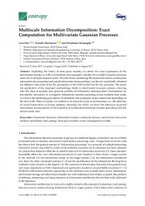
There are two sets of internal variables involved in the cap model: the kinematic hardening tensor α and isotropic hardening parameter κ. For detailed formulation as well as material properties fitted to limestone data, the reader is referred to [2, 8]. If a fully implicit integration is chosen, 13 equations comprise the local system of equations to be solved, (5), (6), (7). This number can be reduced to 7 using a modified spectral decomposition method as shown in [2]. Nevertheless, it is still a daunting task to derive the necewsary sensitivities of the tangent operator analytically. To demonstrate the effectiveness of AD in deriving local tangent, we perform two sets of single element tests: (1) plane strain compression with loading and unloading, and (2) plane stress compression followed by shear loading. Benchmark solutions using analytically derived sensitivities, as see in [2], will be used to verify the solutions obtained using AD. Additionally, integration using an explicit algorithm will be used for comparison purposes. For the plane strain compression with loading and unloading, Figure 1(a) shows the stressstrain response of the implicit AD algorithm, explicit AD algorithm and benchmark solutions using the analytical tangent. It can be seen that both implicit and explicit implementations match the benchmark solutions very well. Also, we report the convergence profiles using the AD computed tangent at two different strain levels (Points A and B as shown in Figure 1(b)). Quadratic convergence is observed for both strain levels, verifying that the correct local consistent tangent operator is obtained using AD. 0

150

−5

B

A

Point A Point B

10 0

|R|/|R |

Axial Stress, MPa

200

10

Implicit Explicit Benchmark

d

100

−10

10

50

0 0

−15

0.005

0.01 0.015 Axial Strain

(a)

0.02

0.025

10

1

2

3 Iteration Number

4

5

(b)

Figure 1: Plain strain compression with loading and unloading for the cap model. (a) Stress and strain relation. Points A and B show where the convergence profiles are reported. The normal displacement on the darker faces are prescribed to be zero (plane strain condition). (b) Convergence of local residual. |R| is the residual norm and |R0 | is the residual norm at the beginning of the iteration. The second test using the cap model is a plane stress compression test followed by shear loading. Similar to the previous test, we compare implicit AD and explicit AD algorithms against benchmark solutions where an analytical tangent is used. Figure 2(a) shows the stress-strain relation. Both implicit and explicit implementations correctly reproduce the benchmark solutions. For the convergence profiles of the implicit AD algorithm, we pick one point (A) during the compression phase and one point (B) during the shearing phase of the

loading. The results are reported in Figure 2(b). Again, we obtain the expected quadratic convergence behavior. 0

10

120 100

Point A Point B

Uniaxial A

dc > 0

0

|R|/|R |

Stress, MPa

−5

10

80 dc = 0

60 40

Implicit Explicit Benchmark

20

B

ds > 0

−10

10

Shear

0 0

−15

0.01

0.02 Strain

0.03

0.04

10

1

2

3 Iteration Number

(a)

4

5

(b)

Figure 2: Plain stress compression followed by shear loading on cap model. (a) Stress and strain relation. Points A and B show where the convergence profiles are reported. The darker faces are stress-free (plane stress condition). (b) Convergence of local residual. |R| is the residual norm and |R0 | is the residual norm at the beginning of the iteration. For the second numerical example, we will demonstrate the performance of the ADcomputed local tangent on a large-deformation hydride model for modeling used fuel cladding possessing both circumferential and radial hydride responses [1]. The model is formulated within a hyperelasto-plastic large deformation framework, where the mechanical response (stress) of the material is derived from a stored potential energy function as follows Ψ(C) =fm (1 − ξm )Ψ0m (C) n X + fi (1 − ξi )Ψ0i (C, M i ),

(12)

i

where C is the right Cauchy-Green tensor, and M i is the direction vector for the ith hydride. In this example, we investigated the performance of the AD technique in the context of a boundary value problem, where ring compression tests on HB Robinson fuel samples were simulated. Due to symmetry, only a quarter of the ring needs to be modeled. Figure 3(a) shows the finite element mesh and boundary conditions and Figure 3(b) shows the contour of radial damage predicted by the model. To illustrate the convergence using the AD technique on this boundary value problem, we picked two representative elements, one at the bottom right corner (element A in Figure 3(a)) and one at the upper left corner (element B in Figure 3(a)). For each of these two elements, we selected the first integration point to report the convergence profile at two different applied displacement levels d = 3.8 × 10−4 m and d = 4.5 × 10−4 m. Figure 4 shows the convergence profiles for elements A and B. Using the AD-computed tangent, we observed quadratic convergence for both elements. The local iteration process converges within 4 steps.

apply vertical displacement original

Element B to report convergence

deformed

Element A to report convergence

(a)

(b)

Figure 3: Ring compression tests on large-deformation hydride model. (a) Finite element mesh and boundary conditions (elements picked to report convergence profiles are highlighted); (b) Damage accumulation in radial hydrides at applied displacement d = 4.5 × 10−4 m. 5

0

10

10

Element A Element B

Element A Element B

0

10

−5

0

|R|/|R |

|R|/|R0|

10 −5

10

−10

10 −10

10

−15

10

1

−15

1.5

2 2.5 3 Iteration Number

3.5

4

10

(a)

1

1.5

2 2.5 Iteration Number

3

(b)

Figure 4: Convergence profiles at Elements A and B for a ring compression test using a large deformation hydride model. Applied displacements are (a) d = 3.8e−4 m, and (b) d = 4.5e−4 m. Conclusions In this paper, we propose a numerically exact approach based on automatic differentiation for computing the sensitivities used in the construction of the local tangent operators in small- and large-deformation constitutive models. These tangent operators are essential for achieving the desired local convergence rate when Newton-type iterative methods are used in solving nonlinear equations in integrating constitutive models. The AD algorithm works by automating the process of differentiating a series of basic differential formulas using the

chain rule. The AD technique is model-independent. In the numerical examples, two reasonably sophisticated models demonstrating both small- and large-deformation regimes are implicitly integrated, where AD is utilized to provide the derivatives neccesary for constitent Newton iteration. Results of various boundary value problems show that the AD-computed tangent operators provide excellent convergence rates in solving the local nonlinear system of equations. References [1] Q. Chen, J.T. Ostien, and G. Hansen. Development of a used fueal cladding damage model incorporating circumferential and radial hydride responses. Journal of Nuclear Materials, 2013(in review). [2] C. D. Foster, R. A. Regueiro, A. F. Fossum, and R. I. Borja. Implicit numerical integration of a three-invariant, isotropic/kinematic hardening cap plasticity model for geomaterials. Computer Methods in Applied Mechanics and Engineering, 194:5109–5138, 2005. [3] Andreas Griewank and Andrea Walther. Evaluating derivatives: principles and techniques of algorithmic differentiation. Siam, 2008. [4] Christian Miehe. Numerical computation of algorithmic (consistent) tangent moduli in large-strain computational inelasticity. Computer methods in applied mechanics and engineering, 134(3):223–240, 1996. [5] Roger P Pawlowski, Eric T Phipps, and Andrew G Salinger. Automating embedded analysis capabilities and managing software complexity in multiphysics simulation, part i: Template-based generic programming. Scientific Programming, 20(2):197–219, 2012. [6] A. Salinger et al. Albany website. https://software.sandia.gov/albany, 2013. [7] Juan C Simo and Robert L Taylor. Consistent tangent operators for rate-independent elastoplasticity. Computer methods in applied mechanics and engineering, 48(1):101–118, 1985. [8] W. Sun, Q. Chen, and J.T. Ostien. Modeling the hydro-mechanical responses of strip and circular punch loadings on water-saturated collapsible geomaterials. Acta Geotechnica, 2013 (in press). doi: 10.1007/s11440-013-0276-x. [9] Xuxin Tu, Jose E. Andrade, and Qiushi Chen. Return mapping for nonsmooth and multiscale elastoplasticity. Computer Methods in Applied Mechanics and Engineering, 198:2286 – 2296, 2009.