Exact and Approximate Methods for the Computation of the Spectral ...

Exact and Approximate Methods for the Computation of the Spectral Stability of Traveling-Wave Solutions

Christopher W. Curtis

A dissertation submitted in partial fulfillment of the requirements for the degree of

Doctor of Philosophy

University of Washington

2009

Program Authorized to Offer Degree: Applied Mathematics

University of Washington Graduate School

This is to certify that I have examined this copy of a doctoral dissertation by Christopher W. Curtis and have found that it is complete and satisfactory in all respects, and that any and all revisions required by the final examining committee have been made.

Chair of the Supervisory Committee:

Bernard Deconinck

Reading Committee:

Robert E. O’Malley Jr. J. Nathan Kutz Anne Greenbaum Yua Yuan

Date:

University of Washington Abstract

Exact and Approximate Methods for the Computation of the Spectral Stability of Traveling-Wave Solutions Christopher W. Curtis Chair of the Supervisory Committee: Associate Professor Bernard Deconinck Applied Mathematics

This thesis addresses the use of various techniques in functional analysis applied to the problem of determining the spectral stability of a traveling wave solution to a nonlinear partial differential equation. This work is separated into two parts. In the first part, a numerical method for the determination of spectral stability, called Hill’s Method, is analyzed. In the second part, I determine, both analytically and numerically, the spectral stability of a family of solitary wave solutions to a new Boussinesq approximation to the Euler water wave equations.

TABLE OF CONTENTS

Page List of Figures . . . . . . . . . . . . . . . . . . . . . . . . . . . . . . . . . . . . . . . .

ii

Chapter 1: Introduction . . . . . . . . . . . . . . . . . 1.1 Traveling Wave Solutions and Stability . . . . . . 1.2 Hill’s Method . . . . . . . . . . . . . . . . . . . . 1.3 Spectral Stability of a Boussinesq Approximation

. . . .

. . . .

. . . .

. . . .

. . . .

. . . .

. . . .

. . . .

. . . .

. . . .

. . . .

. . . .

. . . .

. . . .

. . . .

. . . .

1 1 6 9

Chapter 2: Hill’s Method . . . . . . . . 2.1 The Floquet-Bloch Decomposition 2.2 The Fourier Decomposition . . . . 2.3 Finite-Dimensional Projection . . .

. . . .

. . . .

. . . .

. . . .

. . . .

. . . .

. . . .

. . . .

. . . .

. . . .

. . . .

. . . .

. . . .

. . . .

. . . .

. . . .

13 14 15 16

. . . .

. . . .

. . . .

. . . .

. . . .

. . . .

. . . .

. . . .

Chapter 3: Proof of Convergence . . . . . . . . . . . . . . . . . . . . . . . . . . . . 18 3.1 Proof of the No-Spurious-Modes Condition . . . . . . . . . . . . . . . . . . . 18 3.2 Proof of the Second Condition . . . . . . . . . . . . . . . . . . . . . . . . . . 26 Chapter 4:

Convergence of Eigenfunctions

. . . . . . . . . . . . . . . . . . . . . . 29

Chapter 5:

Rate of Convergence . . . . . . . . . . . . . . . . . . . . . . . . . . . . 32

Chapter 6: The Boussinesq Approximation . . . . . . . . . . . . . . . . . . . . . . 36 6.1 Linearization and Spectral Problem . . . . . . . . . . . . . . . . . . . . . . . . 36 6.2 Spectral Stability of Elevation Soliton . . . . . . . . . . . . . . . . . . . . . . 37 Appendix A: . . . . . . . . . . . . . . . . . . . . . A.1 Matrix Entries . . . . . . . . . . . . . . . . A.2 The Hyperbolicity of A(Ω, η0 , ρ) . . . . . . . A.3 Results about the Characteristic Polynomial A.4 Asymptotics for σ(A(Ω, η0 , ρ)) . . . . . . . .

. . . . . . . . . . . . . . . . . . . . . . . . of A(Ω, η0 , ρ) . . . . . . . .

. . . . .

. . . . .

. . . . .

. . . . .

. . . . .

. . . . .

. . . . .

. . . . .

. . . . .

. . . . .

. . . . .

44 44 45 46 48

Bibliography . . . . . . . . . . . . . . . . . . . . . . . . . . . . . . . . . . . . . . . . . 51 i

LIST OF FIGURES

Figure Number

Page

1.1

. . . . . . . . . . . . . . . . . . . . . . . . . . . . . . . . . . . . . . . . . . . .

6.1

. . . . . . . . . . . . . . . . . . . . . . . . . . . . . . . . . . . . . . . . . . . . 41

ii

5

ACKNOWLEDGMENTS

I’ll get to thanking people when I’m done writing this thing.

iii

DEDICATION

to my beloved wife, Kate

iv

1

Chapter 1 INTRODUCTION 1.1

Traveling Wave Solutions and Stability

The focus in this thesis is on the stability of traveling-wave solutions (TWS(s)) to evolution equations, i.e. nonlinear-partial-differential equations of the form ut = F (u)

(1.1)

u(x, 0) = u0 (x), where x ∈ R. A TWS is a solution u to (1.1) of the form u(x, t) = T (ct)u0 (x; c), where c is called the wave speed, and T is a semigroup representing the action of a symmetry of the evolution equation, and by u0 (x; c) we mean some appropriate scaling of the initial condition. As an example we look at the focusing nonlinear Schr¨odinger (NLS) equation: 1 iut = − uxx − u|u|2 . 2

(1.2)

It is well known and easy to show that any solution to NLS is invariant under phase transformations i.e. if u solves NLS then ueis is also a solution for any real valued number s. Thus if we look for solutions of the form w(x)eict , we get the following problem 1 cw(x) = wxx + w|w|2 2

(1.3)

Assume w is real and integrate with respect to w to get the differential equation (wx )2 = −w4 + 2cw2 + d.

(1.4)

If we assume d < 0, c2 − d = 41 , and c = k 2 − 12 , then using the elliptic integral [21] cn

−1

Z

k

(x, k) = kx

(k 2 − s2 )−1/2 ((1 − k 2 )2 + s2 )−1/2 ds,

(1.5)

2

we see that w(x) = kcn(x, k). Thus we can generate the TWS 1

u(x, t) = kcn(x, k)e−i( 2 −k 1

where T (ct) = e−i( 2 −k

2 )t

2 )t

,

(1.6)

.

Another example illustrating the use of a different symmetry is Korteweg de-Vries (KdV) equation ut + uux + uxxx = 0

(1.7)

In this case, it is easy to show that if u(x, t) is a solution to KdV, then u(x + s, t) is also a solution, and thus we look for a TWS of the form u(x, t) = w(x − ct; c) = T (ct)w(x; c). Note, in general one can look at problems with the spatial variable being in any arbitrary dimension. In our case, the spatial variable, x, is restricted to be one-dimensional for ease of presentation. The interest in TWS’s stems both from physical importance and mathematical tractability. In physics, translating profiles have been of interest in a number of fields ranging from fluid dynamics to optics, with the famous sech squared profile of KdV being an excellent example. Of course, a TWS is simply a particular solution to a model of some physical system. Thus the scientist is forced to ask, even if we believe in our model, do we really expect to see a particular solution in nature? The idea of stability addresses this key issue in mathematical modeling. There are several notions of stability, some stronger or weaker than others. The strongest definition of stability referred to in this paper is known as orbital stability and is defined in the following way. One says that a TWS u is stable if for any solution ψ(x, t) with nearby initial conditions to u0 (x), one can at each time t find some phase shift s such that ψ(x, t) is close to u0 (x−ct−s). In more technical terms, we have if for all  > 0 there exists δ > 0 such that if ψ(x, t) is a solution to the evolution equation with initial condition ψ(x, 0) = ψ0 (x) and ||ψ0 (x) − u(x)|| < δ,

(1.8)

inf ||ψ(x, t) − u(x − ct − s)|| < 

(1.9)

then s∈R

3

for t  1. Note, ||·|| is a norm of some Hilbert space, with corresponding inner product . To understand the intuition behind this definition, one can look at the propagation of one-soliton solutions in KdV. Since the amplitude and wave speed are coupled, two onesoliton profiles close in amplitude at t = 0 will necessarily diverge in norm as time increases. Thus one might be inclined to say any soliton solution to KdV is unstable. But it is clear that if two soliton solutions begin near each other, they will remain close in norm modulo an appropriate phase shift at every later time t since KdV will preserve the shapes of the initial profiles. In general, orbital stability is quite difficult to establish since the nonlinearities of the evolution equation prevent any simple understanding of the effects of varying initial conditions. A simpler problem can be defined by way of a TWS T (ct)w(x; c). Plugging this ansatz into (1.1), we get Tc T (ct)w(x; c) = F (T (ct)w(x; c))

(1.10)

and so at t = 0, noting that T (0) = 1, we get Tc w(x; c) = F (w(x; c)). Hence, w becomes a stationary solution of the associated PDE ut = F (u) − Tc u.

(1.11)

Let ψ(x, t) be a solution to (1.11) such that ψ(x, 0) = w(x) + v(x). Then formally we can write ψ(x, t) = w(x) + ˜ v (x, t) + O(2 )

(1.12)

v˜(x, 0) = v(x). Substituting (1.13) into (1.11) and collecting in powers of  generates the linear evolution equation v˜t = DF (w(x))˜ v − Tc v˜

(1.13)

v˜(x, 0) = v(x) We will henceforth refer to the linear operator DF (w(x)) − Tc as Lw . If the spectrum of Lw , σ(Lw ), is contained in the closure of the left-hand side of the complex plane, then u = T (ct)w(x; c) is said to be spectrally stable.

4

While weaker, spectral stability is easier to establish than orbital stability. Unfortunately, spectral stability does not necessarily imply orbital stability. However, in the important case that the evolution equation is Hamiltonian, i.e. ut = JE 0 (u),

(1.14)

0

where J is skew adjoint, and E (u) is the derivative of the Hamiltonian E(u), one can directly connect spectral stability to orbital stability. Letting J be invertible, and u = T (ct)w(x; c), in the seminal paper [16], the authors develop necessary and sufficient conditions for estab00

00

lishing orbital stability based on properties of the spectrum of the operator E (w) − Q (w). Q(w) =

1 2

< J −1 Tc w, w > is a second conserved quantity of the Hamiltonian system gen-

erated by the symmetry used to construct the TWS since Tc = T 0 (0)c, T 0 (0) being the 0

infinitesimal generator of T . Using our previous notation, we have F (u) = JE (u), thus 00

00

00

DF (u) = JE (u) and E (w) − Q (w) = J −1 (DF (w) − Tc ) = J −1 Lw . A great deal of work has been done connecting σ(J −1 Lw ) to σ(Lw ), and it has been shown for a wide class of Hamiltonian problems that spectrally instability implies orbital stability. Further, being able to compute σ(J −1 Lw ) and σ(Lw ) provides key hints as to how to establish orbital stability beyond the cases covered in [16]. As an explicit example to make the previous terminology more concrete and to show a prominent case of a Hamiltonian system, we again use focusing NLS. If we separate u = ψ + iφ, then we get the PDE     ψ 0 −1   =   φ 1 0

1 2 ψxx

+

ψ(φ2

+

ψ2)

t

0 1 2 φxx

0



+

φ(φ2

+

ψ2)



(1.15)

For NLS, Z  E(φ, ψ) = and

 1 2 1 2 2 2 2 − (φx + ψx ) + (φ + ψ ) dx, 2 4 

J= 

0 −1 1

0

(1.16)

 .

(1.17)

It is straightforward to show, where T in this case is the phase shift generating (1.6), that Z c Q(u) = − |u|2 dx. (1.18) 2

5

00

00

Choosing u to be (1.6), E (w) − Q (w) is  

1 2 2 ∂x

+

3w2 (x) 0

+c



0 1 2 2 ∂x

+

w2 (x)

+c



(1.19)

which is just J −1 Lw for focussing NLS. For (1.6), one can approximate σ(Lw ) by way of Hill’s method (explained in the following sections), which for k = .8, produces the plot

Figure 1.1:

which shows that (1.6) is unstable, both spectrally and thus orbitally. As for when the given evolution equation is not Hamiltonian, one still attempts to make use of a knowledge of the spectrum of the associated linearization, but no general theorems exist like those in [16]. Instead, one must make recourse to a number of tools from dynamical systems which are usually infinite dimensional versions of the manifold theorems used in finite-dimensional-dynamical systems. Suffice to say though, establishing the spectral stability of solutions to nonlinear problems is the first step any researcher should take when attempting to determine the orbital stability of said particular solution. Thus, this thesis addresses different means at computing the spectrum of linear operators. These are explained in the following sections.

6

1.2

Hill’s Method

Hill’s method is used to approximate the spectrum of the operator Sp ψ ≡ ∂xp ψ +

p−1 X

fk (x) ∂xk ψ,

(1.20)

k=0

where ψ is in some appropriate space to be defined later. The coefficient functions fk (x) are smooth, T -periodic functions: fk (x + T ) = fk (x), k = 0, . . . , p − 1. This is denoted as fk ∈ C∞ (ST ) .

(1.21)

Using Floquet and Fourier theory, our approximation starts by computing a bi-infinite matrix representing a parameter-dependent symbol of Sp . We make the problem finite dimensional by truncating the bi-infinite matrix in both rows and columns; we then compute the eigenvalues of the resulting finite-dimensional matrix. Such an approach is commonly used. This is made more precise in the following section. In modern terminology, this truncation may be called a Galerkin approximation [3], though it is also called a projection method in [5]. In its full generality, Hill’s method was first developed in [11]. However, the method has appeared in more specialized contexts as early as 1886, when George Hill published [17]. This paper detailed his investigations into the reduced three-body problem, where an analysis of small perturbations led him to seek solutions to the linear problem d2 ψ + dx2

θ0 + 2

∞ X

! θn cos(2nx) φ = 0.

(1.22)

n=1

Here θk , k = 1, 2, . . ., are real parameters. In his analysis, Hill incorporated both Floquet and Fourier theory, which led him to consider infinite-dimensional matrices and their corresponding determinants. Hill used these determinants in a formal way, and he attempted to approximate the spectra of the infinite-dimensional matrices using the spectra of threeby-three truncations. Inspired by Hill’s work, a rigorous theory on determinants of infinite matrices was initiated by Poincar´e [27] and von Koch [32]. This in turn has led to a modern theory of determinants of operators defined over Banach spaces. The treatise by Gohberg, Goldberg, and Krupnick [14] provides an excellent introduction to both the classical origins

7

and modern developments of infinite dimensional determinants, and our work relies heavily on the material in [14] (see also [13] and [6]). However, we do not develop this theory any further. Instead, we focus on proving the validity of Hill’s truncation. This problem, in turn, has its own deep and storied history. A wonderful introduction can be found in [5]. Likewise, in the same reference, one can find a number of examples where using finite-dimensional approximations to compute the spectra of infinite-dimensional operators fails spectacularly. For our problem, however, we show that for general Sp , Hill’s method never converges to spurious eigenvalues in compact domains. In the case that Sp is self-adjoint, we go further and show, again on any compact domain, that Hill’s method converges to the spectrum of Sp restricted to said domain. Further, assuming the convergence of an approximate sequence of eigenvalues to a simple eigenvalue, we show that the corresponding eigenvector approximations converge to a true eigenvector in the L2 -norm. As shown in [11], Hill’s method is exact for constant-coefficient problems. By restricting ourselves to a particular class of self-adjoint operators, which represent the simplest case of non-constant coefficient equations, we show Hill’s method approximates the smallest eigenvalue faster than any polynomial power. This restricted class of operators includes classic problems such as Mathieu’s equation, and it represents a non-trivial and interesting body of problems for which Hill’s method is an excellent approximation scheme. Another, more abstract but also more general, approach for analyzing Hill’s method can be found in the notes of G.M. Vainikko (Chapter 4 of [20]). This approach applies to a more general class of problems than just Hill’s method, and once the approach is mastered, its application to Hill’s method can be viewed as a corollary. The results in [20] not only allow for establishing the convergence of Hill’s method, but the rate of convergence can also be determined. The rate thus found is identical to the one we establish in this paper. In the case of symmetric operators, a convergence proof and rate can also be found in [12]. However, the class of operators considered in [12] is far more restricted than in this paper or [20]. Further, the rate of convergence obtained is far slower than what we or [20] are able to show. The key to the deeper results in [20] is the notion of the aperture between subspaces

8

of a Banach space (see also Chapter 4 of [19]). We make no use of this idea, or any other result found in [20]. Instead, a more direct and explicit approach is used, which may be more natural or intuitive if one is interested in Hill’s method in its own right, as opposed to regarding it as a special case of a more general problem. Indeed, as mentioned above, Hill’s method led to the consideration of determinants of infinite-dimensional operators and the work of [14]. Thus, the methods presented in this paper are new and hopefully insightful. Remarks.

• The form of the operator (1.20) is restrictive in that we equate the coefficient of the highest-order derivative to one. Were the coefficient a constant, this would not change our results. The affect of a non-constant coefficient on our work is non-trivial. However, in many problems (linear stability, scattering) the spectral problems that arise are of the form used here (see the examples in [11]), although variations occur.

• Numerically computing the eigenvalues of a matrix is a nontrivial problem. It is not a problem we consider in this thesis. The sole interest is in the relation between the finite-dimensional approximations as obtained through Hill’s method and the problem they are meant to approximate.

• The work in this paper focuses on spectral problems defined by scalar differential operators (1.20). This restriction is made for ease of presentation. Hill’s method, in essence a Galerkin method, works equally well for systems of equations or for problems with multiple independent variables [11]. Our methods of analysis used apply to the system case, but modifications are necessary for the multi-dimensional case.

• Combining the ideas of Floquet decomposition and the truncation of matrix representations of operators is frequently done when considering periodic operator equations. Three contemporary examples of this can be found in [29], [33], and [34]. Special mention should be made with regards to [34].

9

1.3

Spectral Stability of a Boussinesq Approximation

It has long been a goal of several disciplines to fully understand the Euler surface-water-wave equations, which in scaled form are ∆φ + ∂z2 φ = 0 0 ≤ z < 1 + η(x, y) ∂z φ = 0

z=0

∂t φ + η + 21 (|∇φ|2 + |∂z φ|2 ) = 0

z = 1 + η(x, y)

∂t η + ∇φ · ∇η − 1 ∂z φ = 0

z = 1 + η(x, y)

(1.23)

Here, φ is the velocity potential of an incompressible, irrotational fluid (hence Laplace’s equation on the interior of the fluid), and η is the height of the wave above the resting state of the fluid, which has been scaled to z = 1 in this case. If we denote the unscaled resting height of the fluid as h0 , we have chosen  =

a h0 ,

where a denotes a characteristic amplitude

of the problem. Likewise, we introduce the balance

λ2 h20

=

1 ,

where λ is the magnitude

of the wave vector in the x and y directions. which will allow us to formally derive long wavelength, shallow water approximations to (1.23). In this spirit, as in the derivation of KdV (see [1]), we begin by noting that since φ must be harmonic on the interior of the fluid, we expand φ in z such that φ(x, y, z) =

∞ X

φn (x, y)z n .

(1.24)

n=0

Using the boundary condition at the bottom of the fluid, and substituting our expansion for φ into the scaled Laplace equation of (1.23) and matching powers of z gives  φ(x, y, z) = φ0 (x, y) − ∆φ0 z 2 + O(2 ). 2

(1.25)

Using this expansion, the equations defined at the surface in (1.23) become ηt + ∇ · w + (∇ · (ηw) − 61 ∆∇ · w) = O(2 ) wt + ∇η + ( 21 ∇|w|2 − 12 ∆wt ) = O(2 ),

(1.26)

where w = ∇φ0 . We now introduce the horizontally scaled velocity v given by v=w−

θ2 ∆w + O(2 ) 2

(1.27)

10

where 0 ≤ θ ≤ 1. Formally inverting this equality gives to the order of our approximation w=v+

θ2 ∆v + O(2 ) 2

(1.28)

Substituting this into (1.26), we get 1  ηt + ∇ · v + (∇ · (ηw)) + (θ2 − )∆∇ · w = O(2 ) 2 3 θ2 1 1 2 vt + ∆vt + ∇η + ( ∇|v| − ∆vt ) = O(2 ), 2 2 2

(1.29)

To the first order, we have ηt + ∇ · v = O() vt + ∇η = O(),

(1.30)

and thus we can introduce the formal identities ∆∇ · v = δ∆∇ · v − (1 − δ)∆ηt + O() ∆vt = −µ∆∇η + (1 − µ)∆vt + O().

(1.31)

If we let a = 12 (θ2 − 13 )δ

b = 12 (θ2 − 31 )(1 − δ)

c = 12 (1 − θ2 )µ d = 21 (1 − θ2 )(1 − µ),

(1.32)

and introduce the scalings t x y η w t = √ , (x, y) = ( √ , √ ), η = , w = ,     

(1.33)

and drop all higher order in epsilon terms, we get the following approximation to (1.23) ηt + ∇ · v + ∇ · ηv + a∇ · ∆v − b∆ηt = 0 1 vt + ∇η + ∇|v|2 + c∇(∆η) − d∆vt = 0. 2

(1.34)

The derivation presented here is a summary of that presented in [8] and [4]. There are several interesting aspects of (1.34) that make it an exciting new approximation to (1.23). As pointed out in [8], by varying the coefficients a, b, c, and d, it appears one can capture a variety of phenomena usually associated with separate approximations to the Euler equation. An excellent example of this in practice can be found in [7], where both the second Kadomstev-Petviashvili (KP-II) equation and an associated analog using Benjamin-BonaMahoney (BBM) instead of KdV is derived from (1.34). Thus from [7], we also trivially get BBM and KdV by restricting to one dimension.

11

Another remarkable aspect of (1.34) is that, at least for the parameter values that interest us in this thesis, not only is (1.34) locally well posed, but solutions   of (1.34) will 1 uniformly approximate solutions of (1.23) to O() on timescales of O [4]. Puzzling  though is that (1.34) is only known to be Hamiltonian in the case that b = d. It is not known whether or not (1.34) is Hamiltonian in general. This is an intriguing question given that it is well known that the Euler-water-wave equations are Hamiltonian. Thus if it were the case that (1.34) were not Hamiltonian, it would provide an example where formal multiple scale arguments destroyed the Hamiltonian structure of the parent problem, but which had no bearing on the problem being a valid approximation to said parent problem. It is worth noting that a conserved quantity is found in [4] for cases where b 6= d, so perhaps mathematically it is not troublesome to approximate one conservative system with another. However, physically, Hamiltonicity is considered so important that one would not believe non-Hamiltonian versions of (1.34) could ever be a useful model of (1.23). This issue is not addressed in this thesis. Instead, we attempt to prove the spectral stability of sech2 solutions to (1.34). In particular we look at solutions of the form

η0 sech2 (λξ) , r 3 v1 = η0 sech2 (λξ) η0 + 3 v2 = 0 η=

(1.35) (1.36) (1.37)

This is a very natural place to begin assessing the phenomenological accuracy of (1.34) given the prominence that the sech2 profile has in the subject of water waves. It is known that these profiles are stable for both KdV and KP-II, and there is strong experimental evidence (Hammack and Segur) that they describe the profile of surface waves in shallow water. Thus establishing the stability of such solutions to (1.34) is another key step in determining the Boussinesq approximations’ validity as a physical model. However, given the complexity of (1.34), spectral stability is the best that the author can do at present. Even in the case that (1.34) is known to be Hamiltonian, one does not have direct recourse to the results of [16] and its descendants. Analytically, the author can only establish spectral stability with respect to one-dimensional perturbations. Numerically,

12

we can go much further, and further we also look at particular solutions that look like depression ”solitons” and multi ”solitons”. Note, we use quotes around the word soliton since technically a soliton is a solution to a nonlinear PDE obtained by way of the inverse scattering transform which in turn relies upon the existence of a Lax pair representation of said PDE. Thus no solution of (1.34) is known to be an actual soliton. Soliton is by now though just a quick way to say sech profile.

13

Chapter 2 HILL’S METHOD

In essence Hill’s method combines a Floquet (or Bloch) decomposition with a Fourier expansion so as to reduce the numerical computation of the spectrum of a periodic differential operator to the computation of spectra of a family of (finite-dimensional) matrices. Before continuing, some relevant spaces that will be used throughout the rest of this thesis are defined. Let L2 (ST ) be defined as the completion of C (ST ), the space of T -periodic, continuous functions, with respect to the L2 norm on the interval [−T /2, T /2]. Let en (x) =

e−i2πnx/T √ , T

n ∈ Z,

(2.1)

so that for φ ∈ L2 (ST ), we have the associated Fourier series

φ (x) =

∞ X

φˆn en (x) ,

(2.2)

n=−∞

with 1 φˆn = hφ, en i = √ T

T /2

Z

−T /2

φ(x)e∗n (x)dx.

(2.3)

This allows us to associate with every function φ ∈ L2 (ST ) its Fourier transform

n o∞ φˆ ≡ φˆn

n=−∞

.

(2.4)

We define the Sobolev spaces Hp (ST ) in a similar fashion, and in our paper, we define the norm on Hp (ST ) as ([3], pg. 308) 2 X  2πk 2p 2 ˆ ||φ||22,p ≡ φˆ0 + φk . T |k|>0

(2.5)

14

2.1

The Floquet-Bloch Decomposition

First, we define Sp over the Sobolev space Hp (R), with ) ( p Z X k 2 p |f (x)| dx < ∞ , H (R) = f ∈ L2 (R) | k=0

where

fk

denotes the

k th

(2.6)

R

weak derivative of f . This makes Sp closed and densely defined.

We can likewise turn the operator Sp − λ into a first-order differential operator defined on H1 (R; Cp ), where the notation means that the space H1 (R; Cp ) consists of Cp valued functions with one weak derivative, and for which the function and its derivate have Cp norms that are both in L2 (R) (see [28] for more details). Denote the first-order differential operator as S(x; λ) =

d dx

− B(x; λ), where B(x; λ) is a p × p matrix. By definition,

σ(Sp ) = {λ ∈ C : S(x; λ) does not have a bounded inverse} .

(2.7)

Following [30], we use the following decomposition of σ(Sp ) (see also [9], [24]). • σpt (Sp ) = {λ ∈ C : S(x; λ) is Fredholm with zero index.} • σess (Sp ) = σ(Sp )\σpt (Sp ). Since Sp has only periodic coefficients, we need only compute σess (Sp ) [30]. This reduces to the following problem. Theorem 1. λ ∈ σ(Sp ) if and only if the differential equation du dx

= B(x; λ)u, 0 < x < T (2.8)

u(T ) = eiµT u(0) has a solution for some µ ∈ [0, 2π/T ). Proof. See [30], page 1001. We transform the differential equation in Theorem 1 into dψ dx

˜ λ, µ)ψ, 0 < x < T = B(x; (2.9)

ψ(T ) = ψ(0)

15

˜ λ, µ) = B(x; λ) − iµ. We can then via the transformation ψ(x) = e−iµx u(x). Note, B(x; restate Theorem 1 as Theorem 2. λ ∈ σ(Sp ) if and only if the differential equation dψ ˜ λ, µ)ψ, ψ ∈ H1 (ST ; Cp ) = B(x; dx

(2.10)

has a solution for some µ ∈ [0, 2π/T ). It is easy to show that the pth -order system in Theorem 2 is equivalent to the scalar problem

Spµ φ = λφ, φ ∈ Hp (ST ) ,

(2.11)


Spµ φ = e−iµx Sp eiµx φ .

(2.12)

where

An explicit form for Spµ is found in [11]. Theorem 2 implies that we can write σ(Sp ) as σ(Sp ) =

[

σ(Spµ ).

(2.13)

µ

As implied by (2.11), for each value of µ, σ(Spµ ) consists only of point spectra. We approximate these point sets numerically for a fixed value of µ. 2.2

The Fourier Decomposition

To reduce the problem to linear algebra, we resort to a Galerkin method [3] using the orthonormal basis en given at the beginning of this section. Of course, given any orthonormal basis {ϕj }, we can generate a matrix representation for any linear operator M with entries hM ϕj , ϕk i, (j, k) ∈ Z2 . Our particular choice of basis reflects the boundary conditions of our eigenvalue problem (2.11). We interchangeably refer to the bi-infinite matrix, with entries hSpµ ej , ek i, as the Fourier transform or symbol of the linear operator Spµ . We denote the symbol (or Fourier transform, or bi-infinite matrix representation) of Spµ as Sˆpµ , where the µ (n,m)th entry of Sˆpµ is denoted by Sˆp,nm = hSpµ em , en i. We write the Fourier transform of

our eigenvalue problem (2.11) as

16

ˆ Sˆpµ φˆ = λφ.

2.3

(2.14)

Finite-Dimensional Projection

The last step of Hill’s method requires the introduction of the orthogonal projection operator PN onto the subspace spanned by the Fourier modes from −N to N . The effect of PN applied to a periodic function is truncation of the Fourier series i.e. N X

PN φ(x) =

φˆn en (x) .

(2.15)

n=−N

Likewise, the action of the symbol of PN , PˆN , will give



 PˆN φˆ = n

   0  

|n| > N .

(2.16)

    φˆ |n| ≤ N n

µ,τ via Define the (2N + 1) × (2N + 1) matrix SˆN



.. .

..

.         µˆ ˆ ˆ PN S p PN =   ···        . ..

0

0

µ,τ 0 SˆN

0

0 .. .

. ..



   0      0 ···  ,      0   .. .

(2.17)

µ,τ where the τ emphasizes that SˆN is a truncation of a bi-infinite matrix. As a matter of

17

convention, for any operator A with symbol  .. .         ˆ ˆ ˆ PN APN =   ···        . ..

ˆ we define Aˆτ in the same fashion, namely A, N  .. . . . .    0 0 0      τ ˆ (2.18) 0 AN 0 · · ·  .      0 0 0   .. .. . .

Likewise we introduce the shorthand AˆN = PˆN AˆPˆN . Finally, we define the approximate eigenvalue problem

µ,τ ˆτ SˆN φN = λN φˆτN ,

(2.19)

where the subscript N on λN reinforces the order of the approximation. A more detailed derivation is presented in [11].

18

Chapter 3 PROOF OF CONVERGENCE

By the convergence of Hill’s method, we mean that the following two properties are satisfied. ˆµ,τ 1. For a given sequence {λN }∞ N =1 , λN ∈ σ(SN ), and for any  > 0, there exists an integer M such that any λN , N ≥ M , is in an -neighborhood of some λ ∈ σ(Spµ ). ˆµ 2. For all λ ∈ σ(Spµ ), there exists some sequence {λN }∞ N =1 , λN ∈ σ(SpN ), such that λN → λ. The first condition ensures that Hill’s method is accurate, but it leaves open the possibility that the method may not produce all of σ(Spµ ). Likewise, the second statement ensures that the method will faithfully reproduce all of σ(Spµ ), but it does not rule out that the method will produce spurious information. It is this distinction that leads us to refer to the first condition as the “no-spurious modes” condition. We are able to prove a slightly restricted version of the no-spurious modes condition for any operator Spµ . We modify the condition only by requiring the arbitrary sequence {λN }∞ N =1 to be confined to a compact subset of the complex plane. The second condition is essentially proved in [28], for self-adjoint operators. We have not been able to improve upon this restriction. However, we present the outline of the proof provided in [28] for the sake of completeness. 3.1

Proof of the No-Spurious-Modes Condition

Our proof of the first condition relies upon one major theorem. Before proving this theorem, we need to develop and explain the basic machinery necessary for our proof. First, for notational ease, we define the operator S 1

19


• D S 1 = Hp (ST ), S 1 φ = Spµ φ. We now provide a brief introduction to the theory of determinants of operators on a separable Hilbert Space, say H. This material was developed in [14], and we reproduce it here only for completeness or to clarify some points made in [14]. Let B (H) denote the space of all bounded operators from H into itself. Let F denote the space of finite-rank operators. For our purposes, it is not sufficient to use the operator norm induced by the norm on H, say ||·||. Instead, we need to introduce a new norm ||·||Z , where Z denotes a sub-algebra of B (H) such that F ∩ Z is dense in Z and ||·|| ≤ C ||·||Z ,

(3.1)

where C is a constant. Thus Z is an embedded sub-algebra in B (H). Likewise, if the space of finite-rank operators is dense in Z, this implies every element in Z is compact. Next, define the trace of K ∈ F ∩ Z by tr (K) =

n X

λk ,

(3.2)

(1 + λk ) ,

(3.3)

k=1

and define the determinant of I + K as det (I + K) =

n Y k=1

where n is the rank of K and λk are the eigenvalues of K. The issue at hand is whether we can find some continuous function that will serve as an extension of the determinant, which has only been defined on F ∩ Z. A necessary and sufficient condition for this (see [14]) is if the trace is a bounded linear functional in the Z norm, i.e. |tr (K)| ≤ M ||K||Z

(3.4)

holds for all K ∈ F ∩ Z, where M is a constant independent of K. If this condition holds, then for K ∈ Z, we know there exists a sequence of finite-rank operators KN such that lim ||KN − K||Z = 0,

N →∞

(3.5)

and we can define the Z-determinant of I + K as detZ (I + K) = lim det (I + KN ) . N →∞

(3.6)

20

Using the above definitions, one can prove [14]: Theorem 3. (I+K)−1 exists if and only if detZ (I+K) 6= 0. A space well suited for our purposes was developed by Gohberg et al [14]. Define the sub-algebra Ω via:   M  X Ω ≡ A ∈ B (L2 (ST )) : max  lim Aˆnn ,  M →∞

∞ X

ˆ 2 Anm

N |n|>N m=−∞

(3.19)

and X

||PN A(I − PN )||2Ω =

2 X Aˆnm ,

(3.20)

|n|≤N |m|>N

the result follows, since ||A||Ω < ∞. This shows that for A ∈ Ω, we have detΩ (I + A) = lim det (I + PN APN ) ,

(3.21)

  τ det (I + PN APN ) ≡ det IˆN + AˆτN .

(3.22)

N →∞

where

For omitted proofs and more detail on this material the interested reader is advised to consult [14]. Finally, we need two key facts about operators of the form I + K, where I is the identity and K is compact. • I + K is a Fredholm operator. • i (I + K) = 0. Note, for any Fredholm operator F , i(F ) ≡ dim(ker(F )) − dim(ker(F † )),

(3.23)

where F † again denotes the adjoint of F . For proof, see [31]. With these tools in hand, we prove the following theorem. This theorem will be the engine to drive the proof of the no-spurious-mode condition.

23

Theorem 7. Let γ ∈ ρ(S 1 ). Then there exists some constant Mγ such that for N ≥ Mγ , 1,τ γ ∈ ρ(SˆN ).

Proof. Define the operator B : L2 (ST ) → L2 (ST ) via 
−p   2πni ψˆn n 6= 0  T  ˆn= ˆ ψ) (B ,     i−p ψˆ0 n = 0

(3.24)

ˆ is the symbol of B. B, when where ψˆn are the components of the vector ψˆ ∈ l2 , and B applied to S 1 − γ, is introduced to nullify the growth along the diagonal of Sˆ1 − γ. Clearly Hp (ST ) ⊂ R (B). With γ ∈ ρ(S 1 ), we have that S 1 −γ is a bijection from Hp (ST ) to L2 (ST ) ˆ Sˆ1 − γ), noting that by definition. Therefore, we define the operator A whose symbol is B( Hp (ST ) ⊂ R(A). ˆ and (Sˆ1 − γ). Clearly this operator Now consider computing the matrix product of B ˆ and we will show that it is a bounded operator on l2 . Therefore, it is the extension of A, must be the unique bounded extension of Aˆ [28]. We refer to the extension of Aˆ as Aˆ to economize on notation. Given that δnm is the Kroenecker delta function, the terms of Aˆ are then

Aˆnm =

     2πni −p     T   

ip µ +


2πn p T




− γ δnm +

p−1 X

fˆk,n−m i

k

k=0



2πn µ+ T

k ! n 6= 0 .

        

(µp − γ) δ0m +

p−1 X

fˆk,−m µk ik−p n = 0

k=0

(3.25) See [11], equation 17, for an explicit derivation. Therefore, for n 6= 0   1 T  1 ˆ ˆ Ann = 1 + +O pµ − ifp−1,0 , 2π n n2 which shows lim

M →∞

Likewise, we have also shown

M  X

 Aˆnn − 1 < ∞.

(3.26)

(3.27)

n=−M

∞ 2 X ˆ Ann − 1 < ∞. n=−∞

(3.28)

24

For n 6= m and n 6= 0, we have k !2 p−1 X 2πn ˆ fk,n−m µ + T k=0 ! p−1  2k ! 2p p−1 2 X X T 2πn µ + , fˆk,n−m 2πn T

  T 2p ˆ 2 Anm ≤ 2πn ≤

k=0

while for n = 0 we have

(3.29)

k=0

p−1 2 ˆ 2 µ2p − 1 X ˆ fk,−m . A0m ≤ 2 µ −1

(3.30)

k=0

Therefore X m6=n,|n|>0

  2k 2p p−1  2 X X T ˆ µ + 2πn  Anm ≤  2πn T |n|>0 k=0

p−1 ∞ X X ˆ 2 fk,m

! .

(3.31)

m=−∞ k=0

The above shows that 2 X Aˆnm − δnm < ∞,

(3.32)

n,m

and therefore A − I ∈ Ω. Let K = A − I, and so K is compact. It is then clear that A ∈ B (L2 (ST )), and that A is Fredholm. Therefore the range of A is closed. We know Hp (ST ) ⊂ R (A), Hp (ST ) is dense in L2 (ST ), and so together these facts imply R (A) =

L2 (ST ). Hence dim ker A† = 0, and i (A) = 0, so dim (ker (A)) = 0. Therefore A is a bounded bijection from L2 (ST ) to L2 (ST ), which means A has a bounded inverse by the Open Mapping Theorem. Knowing that A has a bounded inverse and that A ∈ Ω, it follows from Theorem 3 that detΩ (A) 6= 0. We have detΩ (A) = lim det (I + PN KPN ) N →∞   τ τ ˆN = lim det IˆN +K , N →∞

(3.33)

  τ +K ˆ τ 6= 0. Since and thus there exists constant Mγ such that for N ≥ Mγ , det IˆN N ˆ=B ˆ PˆN , PˆN B τ ˆ1,τ ˆN AˆτN = B (SN − γ IˆN ),

(3.34)

ˆ T (Sˆ1,τ − γ IˆN ) has trivial kernel. Since B ˆN has trivial kernel, we know which means that B N N that   1,τ ker SˆN − γ IˆN = {0},

(3.35)

25

1,τ and therefore γ ∈ ρ(SˆN − γ IˆN ) for N ≥ Mγ .

Given this theorem, we prove the following corollary. 1,τ Corollary 8. If λNj ∈ σ(SˆN ) and λNj → γ, then γ ∈ σ(S 1 ). j

Proof. Suppose in contradiction that γ ∈ ρ(S 1 ). Then, by Theorem 7, we know for some 1,τ value M that γ ∈ ρ(SˆN ) for N ≥ M . Then

ˆ τ ˆ1,τ ˆ1,τ −1 ˆ τ B ( S − γ)) (SN − γ)−1 = (B N N N 2 2 ˆ τ ˆ1,τ −1 ˆ τ ≤ (B N (SN − γ)) BN 2 2 ˆ τ ˆ1,τ −1 ˆ ≤ (BN (SN − γ)) B . 2

(3.36)

2

ˆ τ . Likewise, per our convention, ˆ T (Sˆ1,τ −γ) = IˆN +K Following the notation in Theorem 7, B N N N ˆ N denote the l2 operator such that K ˆ τ is the (2N +1)×(2N +1) truncation of K ˆ N , and let K N ˆ N = PˆN K ˆ N PˆN = PˆN K ˆ PˆN . From Theorem 7, we know that K is compact, and therefore K ˆ N converges to K in the uniform operator topology. Clearly K ˆτ τ −1 ˆN ˆ N )−1 , ) ≤ (Iˆ + K (IN + K 2

(3.37)

2

and we know that I + K has a bounded inverse. This implies ˆ ˆ −1 ˆ ˆ −1 ˆ −1 ˆ −1 ˆ ˆ ˆ (I + KN ) ≤ (I + K) (I + (I + K) (KN − K)) 2

2

(3.38)

2

ˆ N converges uniformly to K, ˆ there exists L such that (Iˆ + K) ˆ −1 (K ˆ N − K) ˆ < 1/2 Since K 2

for N ≥ L, and therefore ˆ ˆ −1 (K ˆ N − K)) ˆ −1 ≤ 2. (I + (Iˆ + K) 2

(3.39)

Finally, we know that ˆ1,τ −1 ( S − γ) N ≥ 2

1

, 1,τ d γ, σ(SˆN ) 

(3.40)

where 1,τ d(γ, σ(SˆN )) =

inf

1,τ s∈σ(SˆN )

|γ − s| .

(3.41)

26

This implies that 2 1,τ d(γ, σ(SˆN )) ≥ ˆ (Iˆ + K) ˆ −1 B 2

for N ≥ S. Hence, if γ ∈

ρ(S 1 ),

(3.42) 2

1,τ there can be no subsequence λNj ∈ σ(SˆN ) converging to j

γ. Now we can prove the restricted no-spurious-mode condition. Theorem 9. Let D be some compact set in the complex plane, and let {λN }∞ N =1 be a 1,τ sequence contained in D with λN ∈ σ(SˆN ). Then for all  > 0, there exists some integer

M such that λN is in an -neighborhood of some value λ ∈ D ∩ σ(S 1 ) for N ≥ M . Proof. Suppose instead that there exists a subsequence λNj such that d(λNj , D ∩ σ(S 1 )) ≥  > 0. However, since D is compact, λNj must have a convergent subsequence, and this subsequence must converge to some element in σ(S 1 ) by Corollary 8. Hence our original assumption cannot hold, and the theorem is proved. 3.2

Proof of the Second Condition

We were able to prove the first condition under quite general assumptions. Specifically, it was not necessary to impose that S 1 was a self-adjoint operator. We are unable to prove the second condition without making this assumption. However, it should be noted that for non-self-adjoint operators, we have been unable to find numerical examples where the second condition appears not to hold. Our proof relies on a number of results from [28]. To apply these, we need the following lemma. Lemma 10. PN S 1 PN converges strongly to S 1 . Proof. Let ψ ∈ Hp (ST ). Then 1 S ψ − PN S 1 PN ψ = PN S 1 (I − PN ) ψ + (I − PN ) S 1 ψ 2 2 1 ≤ S (I − PN ) ψ 2 + (I − PN ) S 1 ψ 2 ≤ C ||(I − PN ) ψ||2,p + (I − PN ) S 1 ψ 2 . This must become arbitrarily small as N → ∞. Therefore the lemma is proved.

(3.43)

27

The results we need from [28] will now be stated for the sake of completeness. Proofs of the lemmas and theorem can be found in [28], pages 290-292. Definition 11. For any linear operator T, if γ ∈ ρ(T ), the resolvent operator of T is defined as Rγ (T ) ≡ (T − γ)−1 .

(3.44)

Lemma 12. If T is a self-adjoint operator, then

||Rγ (T )||2 =

1 , d(γ, σ(T ))

(3.45)

where d(γ, σ(T )) = inf s∈σ(T ) |γ − s| Lemma 13. If T is self adjoint and Im(γ) 6= 0, then

||Rγ (T )||2 ≤

1 . |Im(γ)|

(3.46)

Definition 14. Given a linear operator T with domain D (T ), a core of T is a subset D ⊂ D (T ) such that T |D = T,

(3.47)

where T |D is the smallest closed extension of T |D . Our operator S 1 is closed over Hp (ST ) [23]. Therefore Hp (ST ) is a core for S 1 . Likewise, each of the finite-rank operators PN S 1 PN is continuous, and consequently, closed on Hp (ST ). This makes Hp (ST ) a common core for S 1 and PN S 1 PN . We can then use Lemma 15. Let PN S 1 PN and S 1 be self-adjoint operators on common core D. If PN S 1 PN converges strongly to S 1 on D, then Rγ (PN S 1 PN ) converges strongly to Rγ (S 1 ) if Im(γ) 6= 0.

Finally, given the above lemma, we use the following theorem. Theorem 16. Let PN S 1 PN and S 1 be self adjoint on common core D. If Rγ (PN S 1 PN ) converges strongly to Rγ (S 1 ) for Im(γ) 6= 0, and if a < b and (a, b) ⊂ ρ(PN S 1 PN ) for N sufficiently large, then (a, b) ⊂ ρ(S 1 ).

28

Proof. See [28], page 290. Theorem 16 can be modified to accommodate subsequences, since the strong convergence of PN S 1 PN to S 1 also holds for subsequences. This lets us prove the second condition. Suppose the second condition were false. This implies that there exists λ ∈ σ(S 1 ) such that 1,τ d(λ, σ(SˆN )) ≥  j

(3.48)

for j sufficiently large. Suppose further that λ 6= 0. This implies that the disc Bλ () = 1,τ ), which implies Bλ (˜ ) ⊂ ρ(PN S 1 PN ), where ˜ ≤ . {z ∈ C : |z − λ| < } is a subset of ρ(SˆN j

Therefore, by Theorem 16, Bλ (˜ ) ⊂ ρ(S 1 ). This is a contradiction, which implies the second condition for λ 6= 0. If λ = 0, we need only pick some c ∈ ρ(S 1 ) and repeat our steps for S 1 − c.

29

Chapter 4 CONVERGENCE OF EIGENFUNCTIONS 1,τ We assume in advance that the approximate eigenvalues, λN ∈ σ(SˆN ), converge to 1,τ some λ ∈ σ(S 1 ). Given λN ∈ σ(SˆN ), there exists a (2N + 1)-dimensional vector φˆτN such

that 1,τ ˆτ τ ˆ ˆ SN φN = λN φN , φˆτN = 1 2

(4.1)

We prove the following proposition. 1,τ ) converges to λ ∈ σ(S 1 ), then there exists a vector φˆ such Theorem 17. If λN ∈ σ(SˆN

that a subsequence of φˆN converges to φˆ in ||·||2 and S 1 φ = λφ. Proof. We extend the vectors φˆτN to vectors φˆN so that PˆN φˆN = φˆN . Given that ||φˆN ||2 = 1, by Alaoglu’s theorem [22] there exists a vector φˆ such that some subsequence of φˆN , denoted ˆ Using the operator B from the proof of Theorem 7, and noting as φˆN , converges weakly to φ. that B commutes with the projection operator PN , we get ˆ φˆN = B ˆ PˆN Sˆ1 PˆN φˆN λN B ˆ Sˆ1 φˆN = PˆN B ˆ φˆN = PˆN (Iˆ + K) ˆ N. = φˆN + PˆN Kφ

(4.2)

B is a compact operator since 2 X  2πn −2p 2 ˆ ˆ ˆ ˆ (B PN − B)ψ ≤ ψˆn T 2 |n|>N   2πN −2p ˆ 2 (4.3) ≤ ψ . T 2   2πN −p ˆ ˆ ˆ This implies that B PN − B ≤ , and so B is a uniform limit of finite-rank T 2 ˆ Likewise, ˆ φˆN → B ˆ φ. operators and is therefore compact. B compact then implies that B

30

ˆ PˆN K ˆ φˆN → K ˆ φ, ˆ →K ˆ uniformly, and since K is compact, we have K ˆ ˆ ˆ ˆ ˆ ˆ ˆ ˆ ˆ ˆ ˆ ˆ ˆ + P K − K ≤ K φ − K φ P K φ − K φ N φ , N N N 2

2

2

2

(4.4)

ˆ Therefore, we have ˆ φˆN → K ˆ φ. which implies PˆN K ˆ ˆ φˆ − K ˆ φ. φˆN → λB

(4.5)

Our weakly convergent sequence φˆN has been shown to converge strongly. This implies ˆ φˆN → φ,

(4.6)

ˆ ˆ φˆ = λB ˆ φ. (Iˆ + K)

(4.7)

and using (4.5)


ˆ is in D S 1 , and We still need to show that the function φ, corresponding to symbol φ, that it is an eigenfunction. There are two cases to consider. The first is λ 6= 0. This implies ˆ is invertible. If Iˆ + K ˆ Sˆ1 is invertible, and we showed in Theorem 7 that the operator Iˆ + K is invertible, then d1 ) = I, ˆ −1 (BS ˆ (Iˆ + K)

(4.8)

d1 denotes the extension of B ˆ Sˆ1 . Likewise, if S 1 is invertible, then for φ ∈ L2 (ST ) where BS ˆ such that Sˆ1 ψˆ = φ. ˆ This implies there must exist some ψ ∈ Hp (ST ), with symbol ψ, ˆ φˆ ˆ −1 B φˆ = λ(Iˆ + K) ˆ −1 B ˆ Sˆ1 ψˆ = λ(Iˆ + K) d1 ψˆ ˆ −1 BS = λ(Iˆ + K) ˆ = λψ,

(4.9)

and therefore φ is an eigenfunction of S 1 .
The second case to consider is λ = 0. In that case let c ∈ ρ S 1 so that the operator S 1 − c is invertible. Repeat the steps for the λ 6= 0 case. If we assume that the eigenvalue λ is simple, then we see that every subsequence of φN converges to some unit multiple of φ since we claimed every sequence of approximate eigenvectors φN has a convergent subsequence. We can then say, upon appropriate rescalings,

31

that the sequence is convergent. The general problem for non-simple eigenvalues appears to be rather difficult, and we do not address it here.

32

Chapter 5 RATE OF CONVERGENCE

Before proceeding, we need two technical lemmas. The first lemma is from [2], page 69. We include the proof for clarity. Lemma 18. If φ ∈ C∞ (ST ), then ||(I − PN )φ||2 = O (N −p ) for all integer values of p > 0.

Proof. Since C∞ (ST ) ⊂ Hp (ST ) for arbitrary p, we can write ||(I −

PN )φ||22

X 2 = φˆn |n|>N

2p X   2πN 2p ˆ 2 = φn T |n|>N 2p X    2πn 2p ˆ 2 T ≤ φn 2πN T |n|>N 2p  T ||φ||22,p . ≤ 2πN 

T 2πN

(5.1)

Therefore
||(I − PN )φ||2 = O N −p , p > 0.

(5.2)

The second lemma relies upon a restriction of the self-adjoint operator S 1 to the form S 1 = ∂xp +

p−1 X

ck ∂xk + f (x),

(5.3)

k=1

where the ci are constants. We denote the constant-coefficient differential operator as Dpµ . This restriction greatly simplifies our work since the operator PN commutes with Dpµ . We now prove our second technical lemma:

33

Lemma 19. If φN and φ are the approximate and true eigenfunctions, respectively, of the operator Dpµ + f (x), then convergence in ||·||2 implies convergence in ||·||2,k for all positive integers k. Proof. We have PN S 1 φN = Dpµ φN + PN f (x)φN . As shown in the previous section, if approximate eigenfunctions φN converge to φ in the ||·||2 norm, then lim ||PN f (x)φN − f (x)φ||2 = 0.

(5.4)

lim Dpµ φN − Dpµ φ 2 = 0,

(5.5)

N →∞

This implies N →∞

which means that φN converges to φ in the graph norm associated with S 1 , i.e. lim

N →∞


||φN − φ||2 + S 1 φN − S 1 φ 2 = 0.

(5.6)

The graph norm associated with the operator S 1 is equivalent to the pth Sobolev norm [23], which implies that lim ||φN − φ||2,p = 0.

N →∞

(5.7)

Convergence in ||·||2,p implies ∂x φN → ∂x φ in ||·||2 , and thus ∂x (Dpµ φN + f (x)φN ) converges to ∂x S 1 φ in ||·||2 . This implies that φN converges to φ in ||·||2,p+1 . Proceeding this way, we see that φN converges to φ in ||·||2,k for all integers k > 0. Finally, we need the following min-max theorem [18]: Theorem 20. Suppose the self-adjoint operator S 1 has least eigenvalue λ0 > −∞. Then λ0 =

inf

||ψ||2 =1



 S 1 ψ, ψ ,

(5.8)

where ψ is understood to be in the domain of S 1 . Using Theorem 20 and our technical lemmas, we prove the next theorem. Theorem 21. Let λ = min σ(S 1 ) > −∞, λ simple. Then there exists a sequence λN → λ, 1,τ λN ∈ σ(SˆN ), and


|λN − λ| = O N −q , q ≥ 1.

(5.9)

34

Proof. By Theorem 20, we have λ=

inf



||ψ||2 =1

 S 1 ψ, ψ .

(5.10)

Define the sequence {λN }∞ N =1 via λN =

D E 1,τ ˆτ ˆτ inf SˆN ψN , ψN , τ ||ψˆN ||2 =1

(5.11)

τ ∈ C2N +1 . Let ψ ˆN denote the extension of ψˆτ , i.e. PˆN ψˆN = ψˆN . We can where ψˆN N

equivalently define λN as λN =

inf

||ψN ||2 =1



 S 1 ψN , ψ N .

(5.12)

This shows that λN ≥ λN +1 ≥ · · · ≥ λ. Since the λN ’s are a monotone sequence, they must ˜ Suppose λ ˜ > λ. Since we know λ ∈ σ(S 1 ) and S 1 is self adjoint, by our have a limit, say λ. 1,τ ) such that second condition for convergence, we know there exists a sequence γN ∈ σ(SˆN

˜ but this would imply that γN < λN , γN → λ. This implies for N large enough that γN < λ, ˜ = λ and λN → λ. which is impossible. Therefore λ Let c > λ1 , c 6= 0. We can alter our definition of λN to λN =



inf

||ψ||2 =1


S 1 PN ψ, PN ψ + c h(I − PN )ψ, ψi .

(5.13)

We introduce this alteration in order to take infimums over the same domain. Let each eigenvalue λN have corresponding eigenvector φN , and let λ have eigenvector φ. We showed in Section 4 that φN → φ in ||·||2 , so we can restrict ourselves to the set EN = {φj }j≥N .

(5.14)

Assume that λ > 0, which implies λN > 0. Consider the difference 1 1 1 1 − = sup 1 − sup . 1 λ λN EN hS ψ, ψi EN (hS PN ψ, PN ψi + c h(I − PN )ψ, ψi)

(5.15)

We have 

 S 1 ψ, ψ = S 1 PN ψ, PN ψ + RN (ψ) ,



 RN (ψ) ≡ (I − PN )ψ, S 1 PN ψ + S 1 ψ, (I − PN )ψ ,

(5.16) (5.17)

35

and so 1 1 1 ≤ sup |−RN (ψ) + c h(I − PN )ψ, ψi| , − λ λN λλN EN

(5.18)

λN − λ ≤ sup |−RN (ψ) + c h(I − PN )ψ, ψi| .

(5.19)

or EN

Using Cauchy-Schwartz,
|RN (ψ) | ≤ S 1 PN ψ 2 + S 1 ψ 2 ||(I − PN )ψ||2 , |c h(I − PN )ψ, ψi | ≤ c ||ψ||2 ||(I − PN )ψ||2 .

(5.20) (5.21)


Given the result of Lemma 19, we bound S 1 PN ψ 2 + S 1 ψ 2 by some constant M . Since EN is closed, there must be some vector φK ∈ EN such that sup |−RN (ψ) + c h(I − PN )ψ, ψi| ≤ (M + c) ||(I − PN )φK ||2 .

(5.22)

EN

Knowing that each φK is smooth, Lemma 18 implies  q T λN − λ ≤ (M + c) ||φK ||2,q 2πN

(5.23)

for all q > 0. Lemma 19 shows that ||φK ||2,q → ||ψ||2,q . So, for a given , there must be some value L such that ||φK ||2,q ≤ (1 + ) ||ψ||2,q for all K ≥ L. Hence, for N ≥ L, we have  λN − λ ≤ (M + c)(1 + )

T 2πN

q ||ψ||2,q .

(5.24)

In the case that λ ≤ 0, pick α such that α + λ > 0. Likewise we see that α+λ= α + λN =

inf



||ψ||2 =1

inf

||ψN ||2 =1

 (S 1 + α)ψ, ψ ,

1  (S + α)ψN , ψN .

(5.25) (5.26)

Then we repeat our argument from above. Note, in the case that inf σ(S 1 ) = −∞, but sup σ(S 1 ) < ∞, we can apply the theorem just proved to the operator −S 1 .

36

Chapter 6 THE BOUSSINESQ APPROXIMATION 6.1

Linearization and Spectral Problem

Again, the Boussinesq system is given by ηt + ∇ · v + ∇ · ηv + a∇ · ∆v − b∆ηt = 0, 1 vt + ∇η + ∇|v|2 + c∇(∆η) − d∆vt = 0. 2

(6.1)

Further, In the case that b ≥ 0 and d ≥ 0, we can rewrite (1.34) to fit our definition of evolution equations as in (1.1). This restriction will be imposed throughout the rest of this thesis, and further a and c will be kept negative and equal. As shown though in [8] and [4], this restriction is not so severe and in fact represents the majority of the physically interesting cases where (1.34) might be used. The spectral stability of traveling line solitary wave solutions under two-dimensional small perturbations (transverse stability) are now studied. In specific, we linearize the system around the solution (η ∗ , u∗ , 0) which is the line (independent of y) traveling solution to (6.1), i,e. η ∗ (x, y, t) = η(ξ),

u∗ (x, y, t) = u(ξ)

with ξ = x − kt. Using the fact ∂t = −k∂ξ + ∂t and let the solution be of the form η(ξ, y, t) = η ∗ + ¯ η (ξ, y, t) u(ξ, y, t) = u∗ + ¯ u(ξ, y, t)

(6.2)

v(ξ, y, t) = 0 + ¯ v (ξ, y, t) By substituting (6.2) into (6.1) and dropping the 2 terms, one obtains the equations for (¯ η, u ¯, v¯) which read (the bars on the dependent variables are dropped for simplicity of

37

notation) − ηt + b∆ηt = −kηξ + bk∆ηξ + ∇ · v + a∇ · ∆v + ∇(η ∗ v + v∗ η)

(6.3)

− vt + d∆vt = −kvξ + dk∆vξ + ∇η + c∇(∆η) + ∇(v · v∗ ) Since the equations are linear, it is natural to consider the solutions with respect to each mode. Assume the solutions are in the form of η(ξ, y, t) = N (ξ, ρ, Ω)eiρy+Ωt + complex conjugate (6.4) v(ξ, y, t) = V(ξ, ρ, Ω)eiρy+Ωt + complex conjugate Substituting (6.4) into (6.3) and denote V = (U, V )t , one obtains the equation

      ∗ ∗ ∗ L 0 0 N iρM2 M2 ∂ξ + ηξ N kL ∂ + uξ + u ∂ξ  1    1 ξ          Ω  0 K1 0   U  =  M1 ∂ξ kK1 ∂ξ + u∗ξ + u∗ ∂ξ 0  U        0 0 K1 V iρM1 iρu∗ kK1 ∂ξ V (6.5) where K1 = d∂ξξ − dρ2 − 1, 2

M1 = c∂ξξ − cρ + 1,

L1 = b∂ξξ − bρ2 − 1, 2

(6.6) ∗

M2 = a∂ξξ − aρ + 1 + η ,

The corresponding eigenvalue problem is finding eigenvalues Ω and corresponding eigenfunctions for each ρ. The study of the case ρ = 0 is associated to the one-dimensional stability of the line solutions and the study of ρ 6= 0 is associated to the transverse stability. 6.2

Spectral Stability of Elevation Soliton

We wish to establish the spectral stability of the elevated soliton like solution η ∗ =η0 sech2 (λξ) , r 3 ∗ sech2 (λξ) , u =η0 η0 + 3

(6.7)

v ∗ =0 for parameter values a = c < 0, b > −a, d > 0,

(6.8)

38

with 2a + b + d = 13 , and 1 λ= 2

s

2η0 3 + 2η0 . , k=p 3(a − b) + 2b(η0 + 3) 3(3 + η0 )

Note, in all subsequent calculations in this section and in the appendix, we substitute −a for a. First, we transform (6.5) into a first-order system     φ φ d   = (A(Ω, η0 , ρ) + iρW (η0 , ρ) + C(ξ, η0 , ρ))  , dξ ψ ψ

(6.9)

where φ = (N, U, N 0 , U 0 , N 00 , U 00 )T , (V, V 0 , V 00 )T ,

ψ= and



(6.10)

A0 (η0 , ρ) + ΩA1 (η0 , ρ)

(6.11)

0

  A(Ω, η0 , ρ) =  

   . 

0

(6.12)

B0 (η0 , ρ) + ΩB1 (η0 , ρ)

The explicit entries in the above matrices are provided in the appendix. While the first-order system is not an eigenvalue problem per se, it is equivalent to our original eigenvalue problem in the following way. Define the operator T (Ω) such that
D (T (Ω)) = H1 R; C9 , d − (A(Ω, η0 , ρ) + C(ξ, η0 , ρ) + iρW (η0 , ρ)) . T (Ω) = dξ

(6.13)

Given some value Ω, if T (Ω) has a bounded inverse then Ω is not in the spectrum of our linearization. Likewise, if T (Ω) does not have a bounded inverse, then Ω is in the spectrum of our linearization. For more details and exposition, see [30]. A means of determining the invertibility of T (Ω) is provided by the theory of exponential dichotomies. Following [10] and [30], we say that T (Ω) generates an exponential dichotomy on R if given the fundamental solution matrix of T (Ω), say X(ξ), there exists a projection operator P , and positive constants K, L, α, and β such that the inequalities X(t)P X −1 (s) ≤ Ke−α(t−s) , for t ≥ s X(t)(I − P )X −1 (s) ≤ Le−β(s−t) , for s ≥ t

(6.14)

39

are satisfied for all values of t and s in R. A result of Palmer ([25], [26]) shows that T (Ω) has a bounded inverse if and only if there exists an exponential dichotomy on R. While such a condition is difficult to show for T (Ω), for the constant-coefficient operator d T˜(Ω) ≡ − A(Ω, η0 , ρ), dξ

(6.15)

T˜(Ω) will have an exponential dichotomy on R if and only if A(Ω, η0 , ρ) is hyperbolic [30]. Thus we might hope to make use of the ”roughness” theorem from [10]. Theorem 22. If the ODE

d dξ

− F (ξ) generates an exponential dichotomy on R, then if the

matrix B(ξ) satisfies the inequality sup ||B|| ≤ ξ∈R

α , 4K 2

where α and K are the constants in (6.14), then

d dξ

(6.16)

− F (ξ) − B(ξ) generates an exponential

dichotomy on R as well. It can be shown (see Appendix, section A.1), that A(Ω, η0 , ρ) is hyperbolic if Re (Ω) 6= 0, which is the region in which we are interested. Then A(Ω, η0 , ρ) has three eigenvalues, say µ1 (Ω, η0 , ρ), µ2 (Ω, η0 , ρ), and µ3 (Ω, η0 , ρ) in the left-hand plane, and each are simple and analytic for Re (Ω) ≥ 0 (see Appendix, Lemma 28). Let Γ denote a smooth, closed curve containing only these eigenvalues, and define the projection associated with the exponential dichotomy for A(Ω) by 1 P (Ω, η0 , ρ) = − 2πi

I

(A(Ω, η0 , ρ) − z)−1 dz.

(6.17)

Γ

This projection can be decomposed into the projections Pi associated with the individual eigenvalues µi . Further, the Pi are mutually orthogonal [19], and so we have (letting the variables Ω, η0 , and ρ be understood) At −As e P e = P1 eµ1 (t−s) + P2 eµ2 (t−s) + P3 eµ3 (t−s) ≤ e−α(Ω,η0 ,ρ)(t−s) , where α(Ω, η0 , ρ) = mini {|Re (µi (Ω, η0 , ρ))|}. This provides the following modification of the “roughness” theorem from [10].

(6.18)

40

Theorem 23. If sup ||C(ξ, η0 , ρ) + iρW (η0 , ρ)|| ≤ ξ∈R

1 α(Ω, η0 , ρ) 4

(6.19)

then T (Ω) will have an exponential dichotomy on R and therefore have a bounded inverse. Hence, if we can control α(Ω, η0 , ρ) for Re (Ω) > 0, we can establish a range of η0 and ρ values satisfying the inequality of Theorem 23 and thus prove spectral stability for the given range of parameter values. Let µ1 (Ω, η0 , ρ) be the eigenvalue in the left-hand plane with smallest real part. We know that µ1 (Ω, η0 , ρ) can never be strictly imaginary (see appendix, Lemma 26), but for Theorem 23 to be useful, we need to find some lower bound on the magnitude of Re (µ1 ). From basic perturbation theory, we know for |Ω|  1 that µ1 (Ω, η0 , ρ) must be within O(Ω) of µ1 (0, η0 , ρ). We can now prove the following theorem. Theorem 24. If Re (Ω) ≥ 0, a, b, d are in some neighborhood of −1/9, 1/3 and 2/9, ρ = 0, and η0 is sufficiently small, then α(Ω, η0 , ρ) ≤ µ1 (0, η0 , 0).

(6.20)

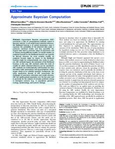
p Proof. From the appendix, we know that µ2 = − ρ2 + 1/d, and so it satisfies (6.23). Therefore, we only need to study the remaining two eigenvalues. From the asymptotic results presented in the appendix, we know there exists constants M and N such that (6.23) holds for |Ω| ≤ M and |Ω| ≥ N . Therefore, we need only establish the inequality in the intermediate region D2 from Figure 1. Given that µ1 (Ω, η0 , ρ) is analytic in the right-half plane, this makes Re (µ1 (Ω, η0 , ρ)) a harmonic function. So, to prove the inequality on D2, we only need to prove it along ∂(D2), and then invoke the maximum principle for harmonic functions. Clearly, by construction, this means we only need to prove the inequality on ∂(D2) ∩ iR. A final simplification can be made by noting that if we let Ω = iω, ω ∈ R, then σ(A(iω)) = σ(A(−iω)), so then one only need prove the bound on ∂(D2) ∩ iR+ . Given the above, denote the characteristic polynomial of A0 + ΩA1 as p(µ). If we show that the associated polynomial b(z) ≡ p(µ1 (0, η0 , 0) + iz)

(6.21)

41

Figure 6.1:

has no real roots in z, then the asymptotic behavior of both µ1 and µ3 as Ω → ∞ guarantees (6.23) must be satisfied. The four eigenvalues of A(Ω, η0 , ρ) are either imaginary or have positive real part (see Lemma 27). This ensures that there can be at most two real roots for b(z). So, we must show that b(z) cannot have a real root. To do this, first let p1 (x) = Re (b(x)), and p2 (x) = Im (b(x)), where x is real. Hence, for b to have real root, p1 and p2 must have a simultaneous root. Thus, we compute the resolvent (see [15] for definition and relevant theorems), R(p1 , p2 ), which is zero if and only if p1 and p2 have a common root. We can compute R(p1 , p2 ) using MAPLE, which gives R(p1 , p2 ) = 64µ61 (0, η0 , 0)(k 2 bd − a2 )ω 2 g(ω, k, µ1 (0, η0 , 0)).

(6.22)

Unfortunately, g is a rather complicated polynomial expression in all of its variables. Thankfully though, µ1 (0, η0 , 0) → 0 and k → 1 as η0 → 0, thus we can expand g as g(ω, k, µ1 (0, η0 , 0)) = 3ω 2 (aw2 + 1)2 g˜(w) + O((k − 1), µ1 (0, η0 , 0)).

(6.23)

Hence, if we show that g˜ is positive for ω > 0, we are done, since we only need to look at values of ω on a finite interval. Of course, even g˜(ω) is difficult to analyze, but if we insert the particular values for a, b, and d as given in the statement of the theorem, we get g˜(ω) =

728 14200 6 5849 4 19718 2 16 ω 10 − ω8 + ω + ω + ω + 15. 1594323 1594323 1594323 177147 19683

(6.24)

42

One can factor

16 10 1594323 ω

−

728 8 1594323 ω

+

14200 6 1594323 ω

into

8ω 6 4 1594323 (2ω

− 91ω 2 + 1775), which

only has a real root at ω = 0. Since 2ω 4 − 91ω 2 + 1775 is positive at the origin, and 5849 4 177147 ω

19718 2 + 19683 ω + 15 is always positive, we see that g˜(ω) > 0, and thus for η0 sufficiently

small, g(ω, k, µ1 (0, η0 , 0)) > 0. Thus p1 and p2 have no common roots and the theorem is proved. To now make use of the roughness theorem for exponential dichotomies, we must estimate the size of C(ξ, η0 , 0). For C, we use the matrix 2-norm, which for an n × n matrix A is ||A||22 =

n X

|aij |2

(6.25)

i,j=1

It is straightforward to show r

α(1 + 4λ2 ) sech(λξ) k 2 bd − a2 α = k 2 d2 + a2 + (kd + a)2 + (kb + a)2 .

||C(ξ, η0 , 0)||2 ≤

η0

(6.26)

√ and hence supξ∈R ||C(ξ, η0 , 0)||2 = O(η0 ). As shown in Lemma 24, |µ1 (0, η0 , 0)| = O( η0 ). Hence, we must necessarily have supξ∈R ||C(ξ, η0 , 0)||2 ≤ |µ1 (0, η0 , 0)|/4 for small η0 .

43

Appendix A

A.1

Matrix Entries





0 I 0     A0 (η0 , ρ) =  0 0 I  ,   0 kZ 0



0

0

0

  A1 (η0 , ρ) =  0 0 0  −Z 0 E

(A.1)

   , 

(A.2)

with     kd(bρ2 + 1) a(dρ2 + 1) kbd ad 1 1  , E =  . Z= 2 2 bd − a2 k bd − a2 k 2 2 a(bρ + 1) kb(dρ + 1) ab kbd

(A.3)

In V , we have    B0 (η0 , ρ) + ΩB1 (η0 , ρ) =  

0 0



1

0

0

  1 . 

− Ωk (ρ2 + d1 ) (ρ2 + d1 )

(A.4)

Ω k

For the constant coefficient coupling dominated by ρ, we have 

0

0

0



    W (η0 , ρ) =  0 0 W1  ,   W2 W3 0

(A.5)

44

with  −1 W1 = 2 k bd − a2







0 0 0 0       0  kd(aρ2 + 1) 0 −kad  , W2 =      −(aρ2 + 1) a(aρ2 + 1) 0 −a2 kd

0 0   0 0    0 0 (A.6)



0   W3 =  0  0

0

0

0 a kd



  0 .  0

Finally we have 

0

0

0



    C(ξ, η0 , ρ) =  C1 C2 C3  ,   C4 0 0 with, dropping the

∗

superscript,



0 0    kduξ kdηξ + auξ  auξ aηξ + kbuξ  0  iρ  C3 = 2  kdη k bd − a2  aη

1 C1 = 2 k bd − a2

A.2

(A.7)

0





  1   , C =   kdu 2 k 2 bd − a2   au   0 0 0 0     0 0 0  , C4 =  0   iρ u 0 0 0 kd

0

0 0



  kdη + au 0 0  ,  aη + kbu 0 0  0   0   0 (A.8)

The Hyperbolicity of A(Ω, η0 , ρ)

We are interested in finding where the matrix A(Ω, η0 , ρ) is hyperbolic, which amounts to computing the spectrum of the constant-coefficient operator 

L1

   0  0

0 K1 0

0

−1 

  0   K1

kL1 ∂ξ

   M1 ∂ξ  0

M1 ∂ξ

0

kK1 ∂ξ

0

0

kK1 ∂ξ

   . 

(A.9)

45

We know that L1 and K1 have bounded inverse on L2 (R), so we can instead study 

k∂ξ   −1 F ≡  K1 M1 ∂ξ  0

L−1 1 M1 ∂ξ

0



  0 .  k∂ξ

k∂ξ 0

(A.10)

We can compute the spectrum of F by taking its Fourier transform, Fˆ (w), and then finding the zeros of det(Fˆ − Ω). We have  ˆ det(F − Ω) = (−ikw − Ω) (−ikw − Ω)2 + w2

(aw2 + aρ2 + 1)2 (bw2 + bρ2 + 1)(dw2 + dρ2 + 1)

 (A.11)

So, we clearly see that iR is in the spectrum of F , but we still need to find the roots of (−ikw − Ω)2 + w2

(aw2 + aρ2 + 1)2 . (bw2 + bρ2 + 1)(dw2 + dρ2 + 1)

(A.12)

If we separate real and imaginary parts we must have Re (Ω)2 − (kw + Im (Ω))2 + w2

(aw2 + aρ2 + 1)2 =0 (bw2 + bρ2 + 1)(dw2 + dρ2 + 1)

Re (Ω) (kw + Im (Ω)) = 0.

(A.13)

If we let Re (Ω) 6= 0, then we must have Im (Ω) = −kw, but then we must also have Re (Ω)2 + w2

(aw2 + aρ2 + 1)2 = 0, (bw2 + bρ2 + 1)(dw2 + dρ2 + 1)

(A.14)

which is impossible. Therefore σ(F ) = iR, and A(Ω, η0 , ρ) is hyperbolic if and only if Re (( Ω, η0 , ρ)) 6= 0. A.3

Results about the Characteristic Polynomial of A(Ω, η0 , ρ)

We will now list a number of lemmas concerning the characteristic polynomial, say pA (µ), of the matrix (6.12). Obviously we can factor this polynomial into the characteristic polynomials for A0 + ΩA1 and B0 + ΩB1 . The eigenvalues for B0 + ΩB1 are ) ( r 1 Ω . ± ρ2 + , d k

(A.15)

46

Denote the characteristic polynomial for A0 + ΩA1 by p(µ; Ω). There is of course no general formula to compute the roots of this polynomial since it is sixth order. However, it is not difficult to show though that p(µ; Ω) = µ2 (k 2 p4 (µ) + p˜4 (µ)) − 2kΩµp4 (µ) + Ω2 p4 (µ),

(A.16)

where p4 (µ) = (bµ2 − (bρ2 + 1))(dµ2 − (dρ2 + 1)) 1 p˜4 (µ) = −a2 (µ2 − (ρ2 + ))2 . a

(A.17)

This allows us to prove: Lemma 25. If Re (Ω) ≥ 0 and Im (Ω) 6= 0, then p(µ; Ω) does not have any real, negative, roots. Proof. Assuming µ ∈ R, then separating p(µ; Ω) = 0 into real and imaginary parts gives µ2 (k 2 p4 (µ) + p˜4 (µ)) − 2kRe (Ω) µp4 (µ) + (Re (Ω)2 − Im (Ω)2 )p4 (µ) = 0 (Re (Ω) − kµ)Im (Ω) p4 (µ) = 0.

(A.18)

We only have one possibility and that is p4 (µ) = 0. This would then imply that µ2 p˜4 (µ) = 0, but this is obviously impossible. We also need: Lemma 26. If Ω is purely imaginary, then the eigenvalues are symmetric about the imaginary axis. Proof. Let p(µ; iω) = 0. Then p(−¯ µ; iω) = p(µ; iω) = 0.

(A.19)

47

A.4 A.4.1

Asymptotics for σ(A(Ω, η0 , ρ)) Small Ω Results

To establish results for |Ω|  1, we start by computing the roots of p(µ; 0), which are   s p  k2 2 2 2 + 2a(k − 1) ± k k (b − d) + 4(a − d)(a − b)  . (A.20) 0, ± ρ2 + 3   2(k 2 bd − a2 ) We can then immediately provide the estimates on µ1 (0, η0 , 0) used in the main text. Lemma 27. |µ1 (0, η0 , 0)| = β=

r

η0 2 2(k bd − 1 1 3(2

a2 )

+ 6a −

(β + O(η0 ))1/2 1 18 (b

(A.21)

− d)2 )

Proof. By performing a Taylor expansion, one has that k =1+

η0 + O(η02 ) 2

which also gives k 2 = 1 + η0 + O(η02 ). As can readily be shown p k2 2 2 2 2 3 + 2a(k − 1) − k k (b − d) + 4(a − d)(a − b) , µ1 (0, η0 , 0) = 2(k 2 bd − a2 ) and so by inserting the expansion in k, k 2 , and using the identity −2a + b + d =

(A.22)

(A.23) 1 3,

the

estimate is obtained. The root at zero is a double root, and we will denote each root as µ5 (0, η0 , ρ) and µ6 (0, η0 , ρ). Let the two negative roots be denoted by µ3 (0, η0 , ρ) and µ1 (0, η0 , ρ), with µ3 (0, η0 , ρ) < µ1 (0, η0 , ρ). There is some question as to what will happen to µ5 (Ω, η0 , ρ) and µ6 (Ω, η0 , ρ) for Re (Ω) > 0. Thankfully, zero is a semi-simple eigenvalue of A0 , and we can use the reduction method of Kato [19]. This gives the expansions p k(bρ2 + 1)(dρ2 + 1) + (1 + aρ2 ) (bρ2 + 1)(dρ2 + 1) µ5 (Ω, η0 , ρ) = Ω + O(Ω2 ), k 2 (bρ2 + 1)(dρ2 + 1) − (1 + aρ2 )2 p k(bρ2 + 1)(dρ2 + 1) − (1 + aρ2 ) (bρ2 + 1)(dρ2 + 1) µ6 (Ω, η0 , ρ) = Ω + O(Ω2 ). (A.24) k 2 (bρ2 + 1)(dρ2 + 1) − (1 + aρ2 )2

48

This shows that for Re (Ω) > 0, the two eigenvalues that begin at the origin move into the right-half plane. Using the same asymptotic methods as above, we also prove the following key lemma. Lemma 28. There exists some M > 0 such that µ1 (Ω, η0 , ρ) and µ3 (Ω, η0 , ρ) satisfy (6.23) for |Ω| ≤ N . Further, µ1 (Ω, η0 , ρ) and µ3 (Ω, η0 , ρ) are analytic for Re (Ω) ≥ 0. Proof. We know that A(Ω, η0 , ρ) has no strictly imaginary eigenvalues for Re (Ω) 6= 0. Thus µ3 (Ω, η0 , ρ) and µ1 (Ω, η0 , ρ) are the only eigenvalues of A0 + ΩA1 in the left-hand plane. Further, since µ3 (Ω, η0 , ρ) and µ1 (Ω, η0 , ρ) are simple at Ω = 0, we know both functions are analytic in Ω about the origin [19]. Let µ1 (Ω, η0 , ρ) = µ1 (0, η0 , ρ) + α1 Ω + O(Ω2 ) µ3 (Ω, η0 , ρ) = µ3 (0, η0 , ρ) + α3 Ω + O(Ω2 ).

(A.25)

We then have (d(µ21 (0) − ρ2 ) + 1)(b(µ21 (0) − ρ2 ) + 1)) p µ21 (0) k 2 (b − d)2 + 4(a − d)(a − b) (d(µ23 (0) − ρ2 ) + 1)(b(µ23 (0) − ρ2 ) + 1)) p α3 = , µ23 (0) k 2 (b − d)2 + 4(a − d)(a − b) α1 = −

(A.26)

and α1 < 0 while α3 > 0. Thus for Ω sufficiently small, (6.23) holds. As for the remainder of the lemma, if Im (Ω) > 0, then for small enough Ω we know Im (µ1 (Ω, η0 , ρ)) < 0 and Im (µ3 (Ω, η0 , ρ)) > 0. By Lemma 26, we see then that neither µ1 (Ω, η0 , ρ) nor µ3 (Ω, η0 , ρ) can ever cross the real axis, and therefore they can never intersect. We can repeat a similar argument for Im (Ω) < 0. Since we need analyticity for Re (Ω) ≥ 0, we still have to examine the case where Ω > 0, which is to say that we need to show that µ1 and µ3 never intersect for Ω > 0. To do this, first note that for real Ω, the roots of p(µ; Ω) must be symmetric with respect to the real axis. Since µ1 and µ3 are simple for small Ω, this means they must be real. Further, because of symmetry, they can only leave the negative real axis if they intersect. We can then look for the positive roots of p(−µ; Ω) using Descartes rule of signs. It is straightforward to show that there can only be an even number of roots, and so therefore the µ1 and µ3 can never intersect for Ω > 0. We are then finished.

49

A.4.2

Large Ω Results

In order to study the behavior of the eigenvalues in the left-hand plane for |Ω|  1, we first introduce the substitution t =

1 Ω.

This transforms the eigenvalue problem (A0 + ΩA1 )φ = µ(Ω)φ

(A.27)

  1 φ. (tA0 + A1 )φ = t µ t

(A.28)

into

Repeating the methods used in the previous section, again see [19], for the eigenvalues with negative real part, we obtain the following expansions. r   1 1 µ1 = − ρ2 + + O b Ω r   1 1 µ3 = − ρ2 + + O d Ω

(A.29)

Thus we see there must exist some value N > 0, such that for |Ω| ≥ N , both µ1 and µ3 will satisfy the inequality (6.23).

50

BIBLIOGRAPHY [1] M. Ablowitz and H. Segur. Solitons and the Inverse Scattering Transform. SIAM, Philadelphia, PN, 1981. [2] K. Atkinson. The Numerical Solution of Integral Equations of the Second Kind. Cambridge University Press, Cambridge, 1997. [3] K. Atkinson and W. Han. Theoretical Numerical Analysis: A Functional Analysis Framework. Springer, New York, NY, 2005. [4] J.L. Bona, T. Colin, and D. Lannes. Long wave approximations for water waves. Arch. Rational Mech. Anal., 178:373–410, 2005. [5] A. B¨ottcher. Infinite matrices and projection methods. In Lectures on Operator Theory and Its Applications, pages 3–72. American Mathematical Society, Providence, RI, 1996. [6] A. B¨ottcher and B. Silbermann. Analysis of Toeplitz Operators. Springer-Verlag, New York, NY, 1990. [7] M. Chen. From Boussinesq systems to KP-type equations. Canadian Applied Mathematics Quarterly, 15:367–373, 2004. [8] M. Chen, J.L. Bona, and J-C. Saut. Boussinesq equations and other systems for smallamplitude long waves in nonlinear dispersive media. part I: Derivation and the linear theory. Journal of Nonlinear Science, 12:283–318, 2002. [9] J.B. Conway. A Course in Functional Analysis. Springer, New York, NY, 2nd edition, 1990. [10] W.A. Coppel. Dichotomies in Stability Theory. Springer, Berlin, 1978. [11] B. Deconinck and J. N. Kutz. Computing spectra of linear operators using the FloquetFourier-Hill method. J. Comput. Phys., 219:296–321, 2006. [12] L.M. Delves and Freeman T.L. Analysis of Global Expansion Methods: Weakly Asymptotically Diagonal Systems. Academic Press, New York, NY, 1981. [13] I. Gohberg, S. Goldberg, and M.A. Kaashoek. Classes of Linear Operators: Vol. I. Birkhauser-Verlag, Basel, 1990.

51

[14] I. Gohberg, S. Goldberg, and N. Krupnick. Traces and Determinants of Linear Operators. Birkhauser-Verlag, Basel, 2000. [15] P.A. Griffiths. Introduction to Algebraic Curves. AMS, 1991. [16] M. Grillakis, J. Shatah, and W.A. Strauss. Stability theory of solitary waves in the presence of symmetry. Journal of Functional Analysis, 74:160–197, 1987. [17] G. W. Hill. On the part of the motion of the lunar perigee which is a function of the mean motions of the sun and moon. Acta Math., 8(1):1–36, 1886. [18] P.D. Hislop and I.M. Sigal. Introduction to Spectral Theory: With Applications to Schr¨ oedinger Operators. Springer, New York, NY, 1996. [19] T. Kato. Perturbation Theory for Linear Operators. Springer-Verlag, New York, N.Y., 2nd edition, 1976. [20] M.A. Krasnosel’skii, G.M. Vainikko, P.P. Zabreiko, Ya. B. Rutitskii, and V. Ya. Stetsenko. Approximate Solution of Operator Equations. Wolters-Noordhoff, Groningen, 1972. [21] D.F. Lawden. Elliptic Functions and Applications. Springer-Verlag, New York, NY, 1989. [22] P.D. Lax. Functional Analysis. Wiley, New York, NY, 2002. [23] J. Locker. Functional Analysis and Two-Point Differential Operators. Longman Scientific and Technical, New York, NY, 1986. [24] A.W. Naylor and G.R. Sell. Linear Operator Theory in Engineering and Science. Springer-Verlag, New York, NY, 1982. [25] K.J. Palmer. Exponential dichotomies and transversal homoclinic points. Journal of Differential Equations, pages 225–256, 1984. [26] K.J. Palmer. Exponential dichotomies and fredholm operators. Proceedings of the American Mathematical Society, pages 149–156, 1988. [27] H. Poincar´e. Sur les d´eterminants d’ordre infini. Bull. Soc. Math. France, 14:77–90, 1886. [28] M. Reed and B. Simon. Methods of Modern Mathematical Physics I, Functional Analysis. Academic Press, New York, NY, 1972.

52

[29] H. Sandberg, E. Mollerstedt, and B. Bernhardsson. Frequency-domain analysis of linear time-periodic systems. IEEE Trans. of Auto. Control, 50:1971–1983, 2005. [30] B. Sandstede. Stability of traveling waves. In B. Fiedler, editor, Handbook of Dynamical Systems, VOL. 2, pages 983–1055. Elsevier Science B.V., 2002. [31] M. Schechter. Principles of Functional Analysis. American Mathematical Society, Providence, RI, 2nd edition, 2001. [32] H. Von Koch. Sur les syst`emes d’une infinit´e d’´equations lin´eaires `a une infinit´e d’inconnues. C. R. Cong. d. Math. Stockholm, pages 43–61, 1910. [33] J. Zhou. Zeros and poles of linear continuous-time periodic systems: Definitions and properties. IEEE Trans. of Auto. Control, 53:1998–2011, 2008. [34] J. Zhou, T. Hagiwara, and M. Araki. Spectral characteristics and eigenvalues computation of the harmonic state operators in continuous-time periodic systems. Systems and Control Letters, 53:141–155, 2004.