Automatic Emotion Prediction of Song Excerpts - Semantic Scholar

NNMR_A_292950

sankarr 18/4/08 15:46

(XML)

Journal of New Music Research 2007, Vol. 36, No. 4, pp. 283–301

Automatic Emotion Prediction of Song Excerpts: Index Construction, Algorithm Design, and Empirical Comparison Karl F. MacDorman, Stuart Ough and Chin-Chang Ho School of Informatics, Indiana University, USA

Abstract Music’s allure lies in its power to stir the emotions. But the relation between the physical properties of an acoustic signal and its emotional impact remains an open area of research. This paper reports the results and possible implications of a pilot study and survey used to construct an emotion index for subjective ratings of music. The dimensions of pleasure and arousal exhibit high reliability. Eighty-five participants’ ratings of 100 song excerpts are used to benchmark the predictive accuracy of several combinations of acoustic preprocessing and statistical learning algorithms. The Euclidean distance between acoustic representations of an excerpt and corresponding emotion-weighted visualizations of a corpus of music excerpts provided predictor variables for linear regression that resulted in the highest predictive accuracy of mean pleasure and arousal values of test songs. This new technique also generated visualizations that show how rhythm, pitch, and loudness interrelate to influence our appreciation of the emotional content of music.

1. Introduction The advent of digital formats has given listeners greater access to music. Vast music libraries easily fit on computer hard drives, are accessed through the Internet, and accompany people in their MP3 players. Digital jukebox applications, such as Winamp, Windows Media Player, and iTunes offer a means of cataloguing music collections, referencing common data such as artist, title, album, genre, song length, and publication year. But as libraries grow, this kind of information is no longer

enough to find and organize desired pieces of music. Even genre offers limited insight into the style of music, because one piece may encompass several genres. These limitations indicate a need for a more meaningful, natural way to search and organize a music collection. Emotion has the potential to provide an important means of music classification and selection allowing listeners to appreciate more fully their music libraries. There are now several commercial software products for searching and organizing music based on emotion. MoodLogic (2001) allowed users to create play lists from their digital music libraries by sorting their music based on genre, tempo, and emotion. The project began with over 50,000 listeners submitting song profiles. MoodLogic analysed its master song library to ‘‘fingerprint’’ new music profiles and associate them with other songs in the library. The software explored a listener’s music library, attempting to match its songs with over three million songs in its database. Although MoodLogic has been discontinued, the technology is used in AMG’s product Tapestry. Other commercial applications include All Media Guide (n.d.), which allows users to explore their music library through 181 emotions and Pandora.com, which uses trained experts to classify songs based on attributes including melody, harmony, rhythm, instrumentation, arrangement, and lyrics. Pandora (n.d.) allows listeners to create ‘‘stations’’ consisting of similar music based on an initial artist or song selection. Stations adapt as the listener rates songs ‘‘thumbs up’’ or ‘‘thumbs down.’’ A profile of the listener’s music preferences emerge, allowing Pandora to propose music that the listener is more likely to enjoy. While not an automatic process of classification, Pandora offers listeners song groupings based on both their own pleasure ratings and expert feature examination.

Correspondence: Karl F. MacDorman, Indiana University School of Informatics, 535 West Michigan Street, Indianapolis, IN 46202, USA. DOI: 10.1080/09298210801927846 Ó 2007 Taylor & Francis

284

Karl F. MacDorman et al.

As technology and methodologies advance, they open up new ways of characterizing music and are likely to offer useful alternatives to today’s time-consuming categorization options. This paper attempts to study the classification of songs through the automatic prediction of human emotional response. The paper contributes to psychology by refining an index to measure pleasure and arousal responses to music. It contributes to music visualization by developing a representation of pleasure and arousal with respect to the perceived acoustic properties of music, namely, bark bands (pitch), frequency of reaching a given sone (loudness) value, modulation frequency, and rhythm. It contributes to pattern recognition by designing and testing an algorithm to predict accurately pleasure and arousal responses to music. 1.1 Organization of the paper Section 2 reviews automatic methods of music classification, providing a benchmark against which to evaluate the performance of the algorithms proposed in Section 5. Section 3 reports a pilot study on the application to music of the pleasure, arousal, and dominance model of Mehrabian and Russell (1974). This results in the development of a new pleasure and arousal index. In Section 4, the new index is used in a survey to collect sufficient data from human listeners to evaluate adequately the predictive accuracy of the algorithms presented in Section 5. An emotion-weighted visualization of acoustic representations is developed. Section 5 introduces and analyses the algorithms. Their potential applications are discussed in Section 6.

2. Methods of automatic music classification The need to sort, compare, and classify songs has grown with the size of listeners’ digital music libraries, because larger libraries require more time to organize them. Although there are some services to assist with managing a library (e.g. MoodLogic, All Music Guide, Pandora), they are also labour-intensive in the sense that they are based on human ratings of each song in their corpus. However, research into automated classification of music based on measures of acoustic similarity, genre, and emotion has led to the development of increasingly powerful software (Pampalk, 2001; Pampalk et al., 2002; Tzanetakis & Cook, 2002; Yang, 2003; Neve & Orio, 2004; Pachet & Zils, 2004; Pohle et al., 2005). This section reviews different ways of grouping music automatically, and the computational methods used to achieve each kind of grouping. 2.1 Grouping by acoustic similarity One of the most natural means of grouping music is to listen for similar sounding passages; however, this is time

consuming and challenging, especially for those who are not musically trained. Automatic classification based on acoustic properties is one method of assisting the listener. The European Research and Innovation Division of Thomson Multimedia worked with musicologists to define parameters that characterize a piece of music (Thomson Multimedia, 2002). Recognizing that a song can include a wide range of styles, Thomson’s formula evaluates it at approximately forty points along its timeline. The digital signal processing system combines this information to create a three-dimensional fingerprint of the song. The k-means algorithm was used to form clusters based on similarities; however, the algorithm stopped short of assigning labels to the clusters. Sony Corporation has also explored the automatic extraction of acoustic properties through the development of the Extractor Discovery System (EDS, Pachet & Zils, 2004). This program uses signal processing and genetic programming to examine such acoustic dimensions as frequency, amplitude, and time. These dimensions are translated into descriptors that correlate to human-perceived qualities of music and are used in the grouping process. MusicIP has also created software that uses acoustic ‘‘fingerprints’’ to sort music by similarities. MusicIP includes an interface to enable users to create a play list of similar songs from their music library based on a seed song instead of attempting to assign meaning to musical similarities. Another common method for classifying music is genre; however, accurate genre classification may require some musical training. Given the size of music libraries and the fact that some songs belong to two or more genres, sorting through a typical music library is not easy. Pampalk (2001) created a visualization method called Islands of Music to represent a corpus of music visually. The method represented similarities between songs in terms of their psychoacoustic properties. The Fourier transform was used to convert pulse code modulation data to bark frequency bands based on a model of the inner ear. The system also extracted rhythmic patterns and fluctuation strengths. Principal component analysis (PCA) reduced the dimensions of the music to 80, and then Kohonen’s self-organizing maps clustered the music. The resulting clusters form ‘‘islands’’ on a two-dimensional map. 2.2 Grouping by genre Scaringella et al. (2006) survey automatic genre classification by expert systems and supervised and unsupervised learning. In an early paper in this area, Tzanetakis and Cook (2002) investigate genre classification using statistical pattern recognition on training and sample music collections. They focused on three features of audio they felt characterized a genre: timbre, pitch, and rhythm. Mel frequency cepstral coefficients (MFCC),

Automatic emotion prediction of song excerpts which are popular in speech recognition, the spectral centroid, and other features computed from the shorttime Fourier transform (STFT) were used in the extraction of timbral textures. A beat histogram represents the rhythmic structure, while a separate generalized autocorrelation of the low and high channel frequencies is used to estimate pitch (cf. Tolonen & Karjalainen, 2000). Once the three feature sets were extracted, Gaussian classifiers, Gaussian mixture models, and knearest neighbour performed genre classification with accuracy ratings ranging from 40% to 75% across 10 genres. The overall average of 61% was similar to human classification performance. In addition to a hierarchical arrangement of Gaussian mixture models (Burred & Lerch, 2003), a number of other methods have been applied to genre classification, including support vector machines (SVM, Xu et al., 2003), unsupervised hidden Markov models (Shao et al., 2004), naı¨ ve Bayesian learning, voting feature intervals, C4.5, nearest neighbour approaches, and rule-based classifiers (Basili et al., 2004). More recently, Kotov et al. (2007) used SVMs to make genre classifications from extracted wavelet-like features of the acoustic signal. Meng et al. (2007) developed a multivariate autoregressive feature model for temporal feature integration, while Lampropoulos et al. (2005) derive features for genre classification from the source separation of distinct instruments. Several authors have advocated segmenting music based on rhythmic representations (Shao et al., 2004) or onset detection (West & Cox, 2005) instead of using a fixed temporal window. 2.3 Grouping by emotion The empirical study of emotion in music began in the late 19th century and has been pursued in earnest from the 1930s (Gabrielsson & Juslin, 2002). The results of many studies demonstrated strong agreement among listeners in defining basic emotions in musical selections, but greater difficulty in agreeing on nuances. Personal bias, past experience, culture, age, and gender can all play a role in how an individual feels about a piece of music, making classification more difficult (Gabrielsson & Juslin, 2002; Liu et al., 2003; Russell, 2003). Because it is widely accepted that music expresses emotion, some studies have proposed methods of automatically grouping music by mood (e.g. Li & Ogihara, 2004; Wieczorkowska et al., 2005; Lu et al., 2006; Yang et al., 2007). However, as the literature review below demonstrates, current methods lack precision, dividing two dimensions of emotion (e.g. pleasure and arousal) into only two or three categories (e.g. high, medium, and low), resulting in four or six combinations. The review below additionally demonstrates that despite this small number of emotion categories, accuracy is also poor, never reaching 90%.

285

Pohle et al. (2005) examined algorithms for classifying music based on mood (happy, neutral, or sad), emotion (soft, neutral, or aggressive), genre, complexity, perceived tempo, and focus. They first extracted values for the musical attributes of timbre, rhythm, and pitch to define acoustic features. These features were then used to train machine learning algorithms, such as support vector machines, k-nearest neighbours, naı¨ ve Bayes, C4.5, and linear regression to classify the songs. The study found categorizations were only slightly above the baseline. To increase accuracy they suggest music be examined in a broader context that includes cultural influences, listening habits, and lyrics. The next three studies are based on Thayer’s mood model. Wang et al. (2004) proposed a method for automatically recognizing a song’s emotion along Thayer’s two dimensions of valence (happy, neutral, and anxious) and arousal (energetic and calm), resulting in six combinations. The method involved extracting 18 statistical and perceptual features from MIDI files. Statistical features included absolute pitch, tempo, and loudness. Perceptual features, which convey emotion and are taken from previous psychological studies, included tonality, stability, perceived pitch height, and change in pitch. Their method used results from 20 listeners to train SVMs to classify 20 s excerpts of music based on the 18 statistical and perceptual features. The system’s accuracy ranged from 63.0 to 85.8% for the six combinations of emotion. However, music listeners would likely expect higher accuracy and greater precision (more categories) in a commercial system. Liu et al. (2003) used timbre, intensity and rhythm to track changes in the mood of classical music pieces along their entire length. Adopting Thayer’s two axes, they focused on four mood classifications: contentment, depression, exuberance, and anxiety. The features were extracted using octave filter-banks and spectral analysis methods. Next, a Gaussian mixture model (GMM) was applied to the piece’s timbre, intensity, and rhythm in both a hierarchical and nonhierarchical framework. The music classifications were compared against four crossvalidated mood clusters established by three music experts. Their method achieved the highest accuracy, 86.3%, but these results were limited to only four emotional categories. Yang et al. (2006) used two fuzzy classifiers to measure emotional strength in music. The two dimensions of Thayer’s mood model, arousal and valence, were again used to define an emotion space of four classes: (1) exhilarated, excited, happy, and pleasure; (2) anxious, angry, terrified, and disgusted; (3) sad, depressing, despairing, and bored; and (4) relaxed, serene, tranquil, and calm. However, they did not appraise whether the model had internal validity when applied to music. For music these factors might not be independent or mutually exclusive. Their method was divided into two stages:

286


model generator (MG) and emotion classifier (EC). For training the MG, 25 s segments deemed to have a ‘‘strong emotion’’ by participants were extracted from 195 songs. Participants assigned each training sample to one of the four emotional classes resulting in 48 or 49 music segments in each class. Psysound2 was used to extract acoustic features. Fuzzy k-nearest neighbour and fuzzy nearest mean classifiers were applied to these features and assigned emotional classes to compute a fuzzy vector. These fuzzy vectors were then used in the EC. Feature selection and cross-validation techniques removed the weakest features and then an emotion variation detection scheme translated the fuzzy vectors into valence and arousal values. Although there were only four categories, fuzzy k-nearest neighbour had a classification accuracy of only 68.2% while fuzzy nearest mean scored slightly better with 71.3%. To improve the accuracy of the emotional classification of music, Yang and Lee (2004) incorporated text mining methods to analyse semantic and psychological aspects of song lyrics. The first phase included predicting emotional intensity, defined by Russell (2003) and Tellegen et al.’s (1999) emotional models, in which intensity is the sum of positive and negative affect. Wavelet tools and Sony’s EDS (Pachet & Zils, 2004) were used to analyse octave, beats per minute, timbral features, and 12 other attributes among a corpus of 500 20 s song segments. A listener trained in classifying properties of music also ranked emotional intensity on a scale from 0 to 9. This data was used in an SVM regression and confirmed that rhythm and timbre were highly correlated (0.90) with emotional intensity. In phase two, Yang and Lee had a volunteer assign emotion labels based on PANAS-X (e.g. excited, scared, sleepy and calm) to lyrics in 145 30 s clips taken from alternative rock songs. The Rainbow text mining tool extracted the lyrics, and the General Inquirer package converted these text files into 182 feature vectors. C4.5 was then used to discover words or patterns that convey positive and negative emotions. Finally, adding the lyric analysis to the acoustic analysis increased classification accuracy only slightly, from 80.7% to 82.3%. These results suggest that emotion classification poses a substantial challenge.

3. Pilot study: constructing an index for the emotional impact of music Music listeners will expect a practical system for estimating the emotional impact of music to be precise, accurate, reliable, and valid. But as noted in the last section, current methods of music analysis lack precision, because they only divide each emotion dimension into a few discrete values. If a song must be classified as either energetic or calm, for example, as in Wang et al. (2004), it is not possible to determine whether one energetic song is

more energetic than another. Thus, a dimension with more discrete values or a continuous range of values is preferable, because it at least has the potential to make finer distinctions. In addition, listeners are likely to expect in a commercial system emotion prediction that is much more accurate than current systems. To design a practical system, it is essential to have adequate benchmarks for evaluating the system’s performance. One cannot expect the final system to be reliable and accurate, if its benchmarks are not. Thus, the next step is to find an adequate index or scale to serve as a benchmark. The design of the index or scale will depend on what is being measured. Some emotions have physiological correlates. Fear (O¨hman, 2006), anger, and sexual arousal, for example, elevate heart rate, respiration, and galvanic skin response. Facial expressions, when not inhibited, reflect emotional state, and can be measured by electromyography or optical motion tracking. However, physiological tests are difficult to administer to a large participant group, require recalibration, and often have poor separation of individual emotions (Mandryk et al. 2006). Therefore, this paper adopts the popular approach of simply asking participants to rate their emotional response using a validated index, that is, one with high internal validity. It is worthwhile for us to construct a valid and reliable index, despite the effort, because of the ease of administering it. 3.1 The PAD model We selected Mehrabian and Russell’s (1974) pleasure, arousal and dominance (PAD) model because of its established effectiveness and validity in measuring general emotional responses (Russell & Mehrabian, 1976; Mehrabian & de Wetter, 1987; Mehrabian, 1995, 1997, 1998; Mehrabian et al. 1997). Originally constructed to measure a person’s emotional reaction to the environment, PAD has been found to be useful in social psychology research, especially in studies in consumer behaviour and preference (Havlena & Holbrook, 1986; Holbrook et al. 1984 as cited in Bearden, 1999). Based on the semantic differential method developed by Osgood et al. (1957) for exploring the basic dimensions of meaning, PAD uses opposing adjectives pairs to investigate emotion. Through multiple studies Mehrabian and Russell (1974) refined the adjective pairs, and three basic dimensions of emotions were established: Pleasure – positive and negative affective states; Arousal – energy and stimulation level; Dominance – a sense of control or freedom to act. Technically speaking, PAD is an index, not a scale. A scale associates scores with patterns of attributes,

287

Automatic emotion prediction of song excerpts whereas an index accumulates the scores of individual attributes. Reviewing studies on emotion in the context of music appreciation revealed strong agreement on the effect of music on two fundamental dimensions of emotion: pleasure and arousal (Thayer, 1989; Gabrielsson & Juslin, 2002; Liu et al. 2003; Kim & Andre`, 2004; Livingstone & Brown, 2005). The studies also found agreement among listeners regarding the ability of pleasure and arousal to describe accurately the broad emotional categories expressed in music. However, the studies failed to discriminate consistently among nuances within an emotional category (e.g. discriminating sadness and depression, Livingstone & Brown, 2005). This difficulty in defining consistent emotional dimensions for listeners warranted the use of an index proven successful in capturing broad, basic emotional dimensions. The difficulty in creating mood taxonomies lies in the wide array of terms that can be applied to moods and emotions and in varying reactions to the same stimuli because of influences such as fatigue and associations from past experience (Liu et al., 2003; Russell, 2003; Livingstone & Brown, 2005; Yang & Lee, 2004). Although there is no consensus on mood taxonomies among researchers, the list of adjectives created by Hevner (1935) is frequently cited. Hevner’s list of 67 terms in eight groupings has been used as a springboard for subsequent research (Gabrielsson & Juslin, 2002; Liu et al., 2003; Bigand et al. 2005; Livingstone & Brown, 2005). The list may have influenced the PAD model, because many of the same terms appear in both. Other studies comparing the three PAD dimensions with the two PANAS (Positive Affect Negative Affect Scales) dimensions or Plutchik’s (1980, cited in Havlena & Holbrook, 1986) eight core emotions (fear, anger, joy, sadness, disgust, acceptance, expectancy, and surprise) found PAD to capture emotional information with greater internal consistency and convergent validity (Havlena & Holbrook, 1986; Mehrabian, 1997; Russell et al. 1989). Havlena and Holbrook (1986) reported a mean interrater reliability of 0.93 and a mean index reliability of 0.88. Mehrabian (1997) reported internal consistency coefficients of 0.97 for pleasure, 0.89 for arousal, and 0.84 for dominance. Russell et al. (1989) found coefficient alpha scores of 0.91 for pleasure and 0.88 for arousal. For music Bigand et al. (2005) support the use of three dimensions, though the third may not be dominance. The researchers asked listeners to group songs according to similar emotional meaning. The subsequent analysis of the groupings revealed a clear formation of three dimensions. The two primary dimensions were arousal and valence (i.e. pleasure). The third dimension, which still seemed to have an emotional character, was easier to define in terms of a continuity–discontinuity or

melodic–harmonic contrast than in terms of a concept for which there is an emotion-related word in common usage. Bigand et al. (2005) speculate the third dimension is related to motor processing in the brain. The rest of this section reports the results of a survey to evaluate PAD in order to adapt the index to music analysis. 3.2 Survey goals Given the success of PAD at measuring general emotional responses, a survey was conducted to test whether PAD provides an adequate first approximation of listeners’ emotional responses to song excerpts. High internal validity was expected based on past PAD studies. Although adjective pairs for pleasure and arousal have high face validity for music, those for dominance seemed more problematic: to our ears many pieces of music sound neither dominant nor submissive. This survey does not appraise content validity: the extent to which PAD measures the range of emotions included in the experience of music. All negative emotions (e.g. anger, fear, sadness) are grouped together as negative affect, and all positive emotions (e.g. happiness, love) as positive affect. This remains an area for future research.

3.3 Methods 3.3.1 Participants There were 72 participants, evenly split by gender, 52 of whom were between 18 and 25 (see Table 1). All the participants were students at a Midwestern metropolitan university, 44 of whom were recruited from introductory undergraduate music classes and 28 of whom were recruited from graduate and undergraduate human– computer interaction classes. All participants had at least moderate experience with digital music files. The measurement of their experience was operationalized as their having used a computer to store and listen to music and their having taken an active role in music selection. The students signed a consent form, which outlined the voluntary nature of the survey, its purpose and procedure, the time required, the adult-only age restriction, how the

Table 1. Pilot study participants. Age

Female

Male

18–25 26–35 36–45 45þ

27 4 4 1

25 8 2 1

Subtotal: Total:

36

36 72

288


results were to be disseminated, steps taken to maintain the confidentiality of participant data, the risks and benefits, information on compensation, and the contact information for the principal investigator and institutional review board. The students received extra credit for participation, and a US$100 gift card was raffled. 3.3.2 Music samples Representative 30 s excerpts were extracted from 10 songs selected from the Thomson Music Index Demo corpus of 128 songs (Table 2). The corpus was screened of offensive lyrics. 3.3.3 Procedure Five different classes participated in the survey between 21 September and 17 October 2006. Each class met separately in a computer laboratory at the university. Each participant was seated at a computer and used a web browser to access a website that was set up to collect participant data for the survey. Instructions were given both at the website and orally by the experimenter. The participants first reported their demographic information. Excerpts from the 10 songs were then played in sequence. The volume was set to a comfortable level, and all participants reported that they were able to hear the music adequately. They were given time to complete the 18 semantic differential scales of PAD for a given excerpt before the next excerpt was played. A seven-point scale was used, implemented as a radio button that consisted of a row of seven circles with an opposing semantic differential item appearing at each end. The two extreme points on the scale were labelled strongly agree. The participants were told that they were not under any time pressure to complete the 18 semantic differential scales; the song excerpt would simply repeat until everyone was finished. They were also told that

Table 2. Song excerpts for evaluating the PAD emotion scale. Song title

Artist

Year

Genre

Baby Love Jam for the Ladies Velvet Pants Maria Maria Janie Runaway Inside What It Feels Like for a Girl Angel Kid A Outro

MC Solaar Moby Propellerheads Santana Steely Dan Moby Madonna

2001 2003 1998 2000 2000 1999 2001

Hip Hop Hip Hop Electronic Latin Rock Jazz Rock Electronic Pop

Massive Attack Radiohead Shazz

1997 2000 1998

Electronic Electronic R&B

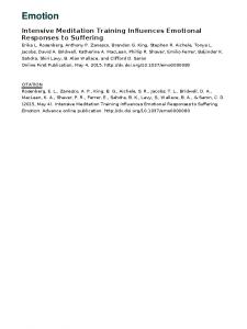
there were no wrong answers. The order of play was randomized for each class. 3.4 Results The standard pleasure, arousal, and dominance values were calculated based on the 18 semantic differential item pairs used by the 72 participants to rate the excerpts from the 10 songs. Although Mehrabian and Russell (1974) reported mostly nonsignificant correlations among the three factors of pleasure, arousal, and dominance, ranging from 70.07 to 70.26, in the context of making musical judgments in this survey, all factors showed significant correlation at the 0.01 level (2-tailed). The effect size was especially high for arousal and dominance. The correlation for pleasure and arousal was 0.33, for pleasure and dominance 0.38, and for arousal and dominance 0.68. In addition, many semantic differential item pairs belonging to different PAD factors showed significant correlation with a large effect size. Those item pairs exceeding 0.5 all involved the dominance dimension (Table 3). In a plot of the participants’ mean PAD values for each song, the dominance value seems to follow the

Table 3. Pearson’s correlation for semantic differential item pairs with a large effect size. D

P

A

Happy Unhappy Pleased Annoyed Satisfied Unsatisfied Positive Negative Stimulated Relaxed Excited Calm Frenzied Sluggish Active Passive

Dominant Submissive

Outgoing Reserved

Receptive Resistant

0.05

0.23**

0.53**

70.14**

0.02

0.59**

70.07

0.11**

0.59**

70.01

0.14**

0.57**

0.61**

0.60**

70.08*

0.58**

0.70**

70.05

0.58**

0.64**

70.04

0.60**

0.73**

0.02

Note: D means Dominance; P means Pleasure; and A means Arousal. Judgments were made on 7-point semantic differential scales (3 ¼ strongly agree; 73 ¼ strongly agree with the opponent adjective). *Correlation is significant at the 0.05 level (2-tailed). **Correlation is significant at the 0.01 level (2-tailed).

289

Automatic emotion prediction of song excerpts arousal value, although the magnitude was less (Figure 1). The standard error of mean pleasure and arousal ratings was 0.06 and 0.04, respectively. In considering the internal reliability of the pilot study, pleasure and arousal both showed high mutual consistency, with a Cronbach’s a of 0.85 and 0.73, respectively. However, the Cronbach’s a for dominance was only 0.64. The percentage of variance explained was calculated by factor analysis, applying the maximum likelihood method and varimax rotation (Table 4). The first two factors account for 26.06% and 22.40% of the variance respectively, while the third factor only accounts for 5.46% of the variance. In considering the factor loadings of the semantic differential item pairs (Table 5), the first factor roughly corresponds to arousal and the second factor to pleasure. The third factor does not have a clear interpretation. The first four factor loadings of the pleasure dimension provided the highest internal reliability, with a Cronbach’s a of 0.91. The first four factor loadings of the arousal dimension also provided the highest reliability, with the same Cronbach’s a of 0.91. 3.5 Discussion The results identified a number of problems with the dominance dimension, ranging from high correlation with arousal to a lack of reliability. The inconsistency in measuring dominance (Cronbach’s a ¼ 0.64) indicated the dimension to be a candidate for removal from the index, because values for Cronbach’s a below 0.70 are generally not considered to represent a valid concept. This was confirmed by the results of factor analysis: a general pleasure–arousal–dominance index with six opponent adjective pairs for each of the three dimensions was reduced to a pleasure–arousal index with four

Fig. 1. Participants’ mean PAD ratings for the 10 songs.

opponent adjective pairs for each of the two dimensions. These remaining factors were shown to have high reliability (Cronbach’s a ¼ 0.91). Given that these results were based on only 10 songs, a larger study with more songs is called for to confirm the extent to which these results are generalizable. (In fact, it would be worthwhile to develop from scratch a new emotion index just for music, though this would be an endeavour on the same scale as the development of PAD.) Nevertheless, the main focus of this paper is on developing an algorithm for accurately predicting human emotional responses to music. Therefore, the promising results from this section were deemed sufficient to provide a provisional index to proceed with the next survey, which collected pleasure and arousal ratings of Table 4. Total variance explained. Extraction sums of squared loadings Component

Total

% of Variance

Cumulative %

1 2 3

4.69 4.03 0.98

26.06 22.40 5.46

26.06 48.46 53.92

Note: Extraction method: Maximum likelihood. Table 5. Rotated factor matrixa. Factor

A. Excited–Calm A. Active–Passive A. Stimulated–Relaxed A. Frenzied–Sluggish D. Outgoing–Reserved D. Dominant–Submissive A. Tense–Placid D. Controlling–Controlled A. Aroused–Unaroused P. Happy–Unhappy P. Positive–Negative P. Satisfied–Unsatisfied P. Pleased–Annoyed D. Receptive–Resistant P. Jovial–Serious P. Contented–Melancholic D. Influential–Influenced D. Autonomous–Guided

1

2

3

0.86 0.85 0.81 0.81 0.76 0.69 0.56 0.43 0.37 0.12 70.01 70.05 70.17 70.15 0.35 0.15 0.13 0.16

0.07 0.12 70.04 0.10 0.14 70.08 70.44 0.00 0.37 0.85 0.85 0.81 0.79 0.62 0.51 0.48 0.13 0.14

0.10 0.16 0.15 0.05 0.24 0.27 70.17 0.40 0.31 0.07 0.13 0.24 0.21 0.42 70.05 0.01 0.37 0.27

Note: P means pleasure; A means arousal; and D means Dominance. Extraction Method: Maximum Likelihood. Rotation Method: Varimax with Kaiser Normalization. a Rotation converged in 5 iterations.

290


100 song excerpts from 85 participants to benchmark the predictive accuracy of several combinations of algorithms. Therefore, in the next survey only eight semantic differential item pairs were used. Because the results indicate that the dominance dimension originally proposed by Mehrabian and Russell (1974) is not informative for music, it was excluded from further consideration. The speed at which participants completed the semantic differential scales varied greatly; from less than two minutes for each scale to just over three minutes. Consequently, this part of the session could range from approximately 20 min to over 30 min. A few participants grew impatient while waiting for others. Adopting the new index would cut by more than half the time required to complete the semantic differential scales for each excerpt. To allow participants to make efficient use of their time, the next survey was self-administered at the website, so that participants could proceed at their own pace.

4. Survey: ratings of 100 excerpts for pleasure and arousal A number of factors must be in place to evaluate accurately the ability of different algorithms to predict listeners’ emotional responses to music: the development of an index or scale for measuring emotional responses that is precise, accurate, reliable, and valid; the collection of ratings from a sufficiently large sample of participants to evaluate the algorithm; and the collection of ratings on a sufficiently large sample of songs to ensure that the algorithm can be applied to the diverse genres, instrumentation, octave and tempo ranges, and emotional colouring typically found in listeners’ music libraries. In this section the index developed in the previous section determines the participant ratings collected on excerpts from 100 songs. Given that these songs encompass 65 artists and 15 genres (see below) and were drawn from the Thomson corpus, which itself is based on a sample from a number of individual listeners, the song excerpts should be sufficiently representative of typical digital music libraries to evaluate the performance of various algorithms. However, a commercial system should be based on a probability sample of music from listeners in the target market.

and arousal associated with different passages in a song (Gabrielsson & Juslin, 2002). However, if the pleasure and arousal associated with a song’s component passages is known, it is much easier to generalize about the emotional content of the entire song. Therefore, the unit of analysis should be participants’ ratings of a segment of a song, and not the entire song. But how do we determine an appropriate segment length? In principle, we would like the segment to be as short as possible so that our analysis of the song’s dynamics can likewise be as fine grained as possible. The expression of a shorter segment will also tend to be more homogeneous, resulting in higher consistency in an individual listener’s ratings. Unfortunately, if the segment is too short, the listener cannot hear enough of it to make an accurate determination of its emotional content. In addition, ratings of very short segments lack ecological validity because the segment is stripped of its surrounding context (Gabrielsson & Juslin, 2002). Given this trade-off, some past studies have deemed six seconds a reasonable length to get a segment’s emotional gist (e.g. Pampalk, 2001, Pampalk et al., 2002), but further studies would be required to confirm this. Our concern with studies that support the possibility of using segments shorter than this (e.g. Peretz, 2001; Watt & Ash, 1998) is that they only make low precision discriminations (e.g. happy–sad) and do not consider ecological validity. So in this section, a 6 s excerpt was extracted from each of 100 songs in the Thomson corpus. 4.2 Survey goals The purpose of the survey was (1)

(2)

(3)

(4)

to determine how pleasure and arousal are distributed for the fairly diverse Thomson corpus and the extent to which they are correlated; to assess interrater agreement by gauging the effectiveness of the pleasure–arousal scale developed in the previous section; to collect ratings from enough participants on enough songs to make it possible to evaluate an algorithm’s accuracy at predicting the mean participant pleasure and arousal ratings of a new, unrated excerpt; to develop a visual representation of how listeners’ pleasure and arousal ratings relate to the pitch, rhythm, and loudness of song excerpts.

4.1 Song segment length An important first step in collecting participant ratings is to determine the appropriate unit of analysis. The pleasure and arousal of listening to a song typically changes with its musical progression. If only one set of ratings is collected for the entire song, this leads to a credit assignment problem in determining the pleasure

4.3 Methods 4.3.1 Participants There were 85 participants, of whom 46 were male and 39 were female and 53 were 18 to 25 years old (see Table 6). The majority of the participants were the same students

Automatic emotion prediction of song excerpts as those recruited in the previous section: 44 were recruited from introductory undergraduate music classes and 28 were recruited from graduate and undergraduate human–computer interaction classes. Thirteen additional participants were recruited from the local area. As before, all participants had at least moderate experience with digital music files. Participants were required to agree to an online study information sheet containing the same information as the consent form in the previous study except for the updated procedure. Participating students received extra credit. 4.3.2 Music samples Six second excerpts were extracted from the first 100 songs of the Thomson Music Index Demo corpus of 128 songs (see Table 7). The excerpts were extracted 90 s into each song. The excerpts were screened to remove silent moments, low sound quality, and offensive lyrics. As a result eight excerpts were replaced by excerpts from the remaining 28 songs.

291

4.3.3 Procedures The study was a self-administered online survey made available during December 2006. Participants were recruited by an email that contained a hyperlink to the study. Participants were first presented with the online study information sheet including a note instructing them to have speakers or a headset connected to the computer and the volume set to a comfortable level. Participants were advised to use a high-speed Internet connection. The excerpts were presented using an audio player embedded in the website. Participants could replay an excerpt and adjust the volume using the player controls while completing the pleasure and arousal semantic differential scales. The opposing items were determined in the previous study: happy–unhappy, pleased–annoyed, satisfied–unsatisfied, and positive–negative for pleasure and stimulated–relaxed, excited–calm, frenzied–sluggish, and active–passive for arousal. The music files were presented in random order for each participant. The time to complete the 100 songs’ 6 s excerpts and accompanying scales was about 20 to 25 min. 4.4 Results

Table 6. Survey participants. Age

Female

Male

18–25 26–35 36–45 45þ

28 5 5 1

25 13 6 2

Subtotal: Total:

39

46 85

Figure 2 plots the 85 participants’ mean pleasure and arousal ratings for the 100 song excerpts. The mean pleasure rating across all excerpts was 0.46 (SD ¼ 0.50), and the mean arousal rating across all excerpts was 0.11 (SD ¼ 1.23). Thus, there were much greater differences in the arousal dimension than in the pleasure dimension. The standard deviation for individual excerpts ranged from 1.28 (song 88) to 2.05 (song 12) for pleasure (M ¼ 1.63) and from 0.97 (song 33) to 1.86 (song 87) for arousal (M ¼ 1.32). The average absolute deviation was calculated for each of the 100 excerpts for both pleasure

Table 7. Training and testing corpus. Genres Rock Pop Jazz Electronic Funk R&B Classical Blues Hip Hop Soul Disco Folk Other Total

Songs

Artists

24 14 14 8 6 6 5 4 4 4 3 3 5

20 12 6 3 2 4 2 3 1 2 2 3 5

100

65

Fig. 2. Participant ratings of 100 songs for pleasure and arousal with selected song identification numbers.

292


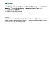
and arousal. The mean of those values was 1.32 for pleasure (0.81 in z-scores) and 1.03 for arousal (0.78 in zscores). Thus, the interrater reliability was higher for arousal than for pleasure. As Figure 3 shows, the frequency distribution for pleasure was unimodal and normally distributed (K-S test ¼ 0.04, p40.05); however, the frequency distribution for arousal was not normal (K-S test ¼ 0.13, p ¼ 0.000) but bimodal: songs tended to have either low or high arousal ratings. The correlation for pleasure and arousal was 0.31 (p ¼ 0.000), which is similar to the 0.33 correlation of the previous survey. The standard error of mean of pleasure and arousal ratings was 0.02 and 0.02, respectively. A representation was developed to visualize the difference between excerpts with low and high pleasure and excerpts with low and high arousal. This is referred to as an emotion-weighted visualization (see Appendix). The spectrum histograms of 100 song excerpts were multiplied by participants’ mean ratings of pleasure in zscores and summed (Figure 4) or multiplied by participants’ mean ratings of arousal and summed (Figure 5). Figure 4 shows that frequent medium-to-loud mid-range

pitches tend to be more pleasurable, while frequent low pitches and soft high pitches tend to be less pleasurable. Subjective pitch ranges are constituted by critical bands in the bark scale. Lighter shades indicate a higher frequency of occurrence of a given loudness and pitch range. Figure 5 shows that louder higher pitches tend to be more arousing than softer lower pitches. Figures 6 and 7 shows the fluctuation pattern representation for pleasure and arousal, respectively. Figure 6 shows that mid-range rhythms (modulation frequency) and pitches tend to be more pleasurable. Figure 7 shows that faster

Fig. 4. The sum of the spectrum histograms of the 100 song excerpts weighted by the participants’ mean ratings of pleasure. Critical bands in bark are plotted versus loudness. Higher values are lighter.

Fig. 3. Frequency distributions for pleasure and arousal. The frequency distribution for pleasure is normally distributed, but the frequency distribution for arousal is not.

Fig. 5. The sum of the spectrum histograms of the 100 song excerpts weighted by the participants’ mean ratings of arousal. Critical bands in bark are plotted versus loudness. Higher values are lighter.

Automatic emotion prediction of song excerpts rhythms and higher pitches tend to be more arousing. These representations are explained in more detail in the next section. 4.5 Discussion The 85 listeners’ ratings of the 100 songs in the Thomson corpus show the pleasure index to be normally distributed but the arousal index to be bimodal. The difference in the standard deviations of the mean pleasure

293

and arousal ratings indicates a much greater variability in the arousal dimension than in the pleasure dimension. For example, the calm–excited distinction is more pronounced than the happy–sad distinction. It stands to reason that interrater agreement would be higher for arousal than for pleasure because arousal ratings are more highly correlated with objectively measurable characteristics of music (e.g. fast tempo, loud). Further research is required to determine the extent to which the above properties characterize music for the mass market in general. The low standard error of the sample means indicates that sufficient data was collected to proceed with an analysis of algorithms for predicting emotional responses to music.

5. Evaluation of emotion prediction method Section 2 reviewed a number of approaches to predicting the emotional content of music automatically. However, these approaches provided low precision, quantizing each dimension into only two or three levels. Accuracy rates were also fairly low, ranging from performance just above chance to 86.3%. The purpose of this section is to develop and evaluate algorithms for making accurate real-valued predictions for pleasure and arousal that surpass the performance of approaches found in the literature. Fig. 6. The sum of the fluctuation pattern of the 100 song excerpts weighted by the participants’ mean ratings of pleasure. Critical bands in bark are plotted versus loudness. Higher values are lighter.

Fig. 7. The sum of the fluctuation pattern of the 100 song excerpts weighted by the participants’ mean ratings of arousal. Critical bands in bark are plotted versus loudness. Higher values are lighter.

5.1 Acoustic representation Before applying general dimensionality reduction and statistical learning algorithms for predicting emotional responses to music, it is important to find an appropriate representational form for acoustic data. The pulse code modulation format of compact discs and WAV files, which represents signal amplitude sampled at uniform time intervals, provides too much information and information of the wrong kind. Hence, it is important to re-encode PCM data to reduce computation and accentuate perceptual similarities. This section evaluates five representations implemented by Pampalk et al. (2003) and computed using the MA Toolbox (Pampalk, 2006). Three of the methods – the spectrum histogram, periodicity histogram, and fluctuation pattern – are derived from the sonogram, which models characteristics of the outer, middle, and inner ear. The first four methods also lend themselves to visualization and, indeed, the spectrum histogram and fluctuation pattern were used in the previous section to depict pleasure and arousal with respect to pitch and loudness and pitch and rhythm. The fifth method, the Mel frequency cepstral coefficients, which is used frequently in speech processing, does not model outer and middle ear characteristics. Pampalk et al. (2003) propose that, to compare acoustic similarity accurately, it is important

294


that the acoustic representation retain audio information related to hearing sensation and not other, extraneous factors. This is one reason why it is good to use the sonogram as a starting point. In addition, visualizations of the sonogram, spectrum histogram, periodicity histogram, and fluctuation pattern are easier for untrained musicians to interpret than visualizations of the MFCC. The sonogram was calculated as follows: (1) 6 s excerpts were extracted 90 s into each MP3 file, converted to PCM format, and down sampled to 11 kHz mono. (2) Amplitude data were reweighted according to Homo sapiens’ heightened sensitivity to midrange frequencies (3–4 kHz) as exhibited by the outer and middle ear’s frequency response (Terhardt, 1979, cited in Pampalk et al., 2003). (3) The data was next transformed into the frequency domain, scaled based on human auditory perception, and quantized into critical bands. These bands are represented in the bark scale. Above 500 Hz, bark bands shift from constant to exponential width. (4) Spectral masking effects were added. Finally, (5) loudness information was converted to sone, a unit of perceived loudness, and normalized so that 1 sone is the maximum loudness value. The sonogram is quantized to a sample rate (time interval) of 86 Hz, the frequency is represented by 20 bark bands, and the loudness is measured in sone. The spectrum histogram counts the number of times the song excerpt exceeds a given loudness level for each frequency band. As with the sonogram, loudness is measured in sone and frequency in bark. Pampalk et al. (2003) report that the spectrum histogram offers a useful model of timbre. The periodicity histogram represents the periodic occurrence of sharp attacks in the music for each frequency band. The fluctuation pattern derives from a perceptual model of fluctuations in amplitude modulated tones (Pampalk, 2006). The modulation frequencies are represented in Hz. The Mel frequency cepstral coefficients define tone in mel units such that a tone that is perceived as being twice as high as another will have double the value. This logarithmic positioning of frequency bands roughly approximates the auditory response of the inner ear. However, MFCC lacks an outer and middle ear model and does not represent loudness sensation accurately. Twenty Mel frequency cepstral coefficients were used in this study. 5.2 Statistical learning methods Even after re-encoding the acoustic signal in one of the above forms of representation, each excerpt is still represented in a subspace of high dimensionality. For example, the fluctuation pattern for a 6 s excerpt has 1200 real-valued dimensions. Thus, past research has often divided the process of categorization into two stages: the first stage reduces the dimensionality of the data while highlighting salient patterns in the dataset.

The second stage performs the actual categorization. A linear model, such as least-squares regression, lends itself to a straightforward statistical analysis of the results from the first stage. It is, therefore, used in this study to compare alternative methods of data reduction. Regression also requires far more observations than predictor variables, especially if the effect is not large (Miles & Shevlin, 2001), which is another reason for dimensionality reduction. The most common method is principal components analysis. The dataset is rotated so that its direction of maximal variation becomes the first dimension, the next direction of maximal variation in the residuals, orthogonal to the first, becomes the second dimension, and so on. After applying PCA, dimensions with little variation may be eliminated. Pampalk (2001) used this method in Islands of Music. However, PCA may offer poor performance for datasets that exhibit nonlinear relations. Many nonlinear dimensionality reduction algorithms, such as nonlinear principal components analysis, are based on gradient descent and thus are susceptible to local minima. Recently, a couple of unsupervised learning algorithms have been developed that guarantee an asymptotically optimal global solution using robust linear decompositions: nonlinear dimensionality reduction by isometric feature mappings (ISOMAP), kernel ISOMAP, and locally linear embedding (LLE). ISOMAP uses Dykstra’s shortest path algorithm to estimate the geodesic distance between all pairs of data point along the manifold (Tenenbaum et al., 2000). It then applies the classical technique of multidimensional scaling to the distance matrix to construct a lower dimensional embedding of the data. LLE constructs a neighbourhood-preserving embedding from locally linear fits without estimating distances between far away data points (Roweis & Saul, 2000). Choi and Choi (2007) develop a robust version of ISOMAP that generalizes to new data points, projecting test data onto the lower dimensionality embedding by geodesic kernel mapping. In addition to this generalization ability, which is based on kernel PCA, kernel ISOMAP improves topological stability by removing outliers. Outliers can wreak havoc with shortest-path estimates by creating short-circuits between distant regions of the manifold. Thus, we chose to compare PCA and kernel ISOMAP, because we believe they are representative of a larger family of linear and nonlinear dimensionality reduction approaches. We also chose to compare these methods to an approach that does not reduce the dimensionality of the acoustic representation of a test excerpt but instead compares it directly to an emotion-weighted representation of all training excerpts – the emotion-weighted visualization of the previous section – as explained later in this section and in the Appendix. This approach

Automatic emotion prediction of song excerpts results in one predictor variable per acoustic representation per emotion. 5.3 Survey goals This section compares the performance of four different methods of automatically estimating a listener’s pleasure and arousal for an unrated song excerpt: (1) nearest neighbour, (2) linear and (3) nonlinear dimensionality reduction and linear model prediction, and (4) distance from an emotion-weighted representation and linear model prediction. Linear dimensionality reduction by principle components analysis is compared with nonlinear dimensionality reduction by kernel ISOMAP to provide predictor variables for multiple linear regression. Hence, this section has two main goals: (1)

(2)

to determine whether continuously valued mean pleasure and arousal ratings of song excerpts can be accurately predicted by automatic means based on previously-rated excepts from other songs; and to determine which combination of dimensionality reduction and statistical learning algorithms provides the highest predictive accuracy.

5.4 Evaluation method of predictive accuracy The jackknife approach (Yang & Robinson, 1986) was used to calculate the average error in the system’s prediction. This was used to calculate the average prediction error for the nearest neighbour method and to compare the performance of PCA and kernel ISOMAP. Regression was performed to calculate the least squares fit of the participants’ mean ratings of pleasure and arousal for the excerpts from all but the first song on the predictor variables for all but the first song. The pleasure and arousal ratings for the first song were then estimated based on the predictor variables for the first song and compared to the participants’ actual mean ratings for the first song. This difference indicated the prediction error for the first song. This process was repeated for the 2nd through the 100th song. Thus, the difference between participants’ actual mean ratings of pleasure and arousal and the ratings predicted using the proposed approach with nearest neighbour, PCA, or kernel ISOMAP could be calculated for all 100 songs. To simplify method comparison, all participant ratings were converted to z-scores, so that prediction error values could also be given in z-scores.

295

determined by the participant mean of the nearest excerpt in a given data representation space. Although various metrics can be used for distance, the L2 norm was chosen (Euclidean distance). For pleasure, the prediction error was 0.48 (in z-scores) in the spectrum histogram space, 0.49 in the periodicity histogram space, 0.52 in the sonogram space and Mel frequency cepstral coefficients space, and 0.54 in the fluctuation pattern space. For arousal, the prediction error was 0.99 in the sonogram space, 0.83 in the spectrum histogram space, 1.26 in the periodicity histogram space, 0.92 in the fluctuation pattern space, and 0.96 in the Mel frequency cepstral coefficients space. The prediction error was also calculated after applying the dimensionality reduction methods, but the results were roughly similar. 5.6 Comparison of PCA and kernel ISOMAP dimensionality reduction Figures 8 and 9 show that nonlinear dimensionality reduction by kernel ISOMAP provides predictor variables that result in slightly more accurate regression estimates of the participant mean for pleasure than linear dimensionality reduction by PCA. Although the figures only list results for subspaces ranging in dimensionality from 1 to 30, prediction error was calculated for all dimensionality N that were not rank deficient (i.e. 1 to 97 for all data representation spaces except periodicity histogram, which was 1 to 4). For pleasure, the prediction error obtained by using PCA was 0.80 (in zscores, N ¼ 1) when applied to the sonograms of the 100 excerpts, 0.81 (N ¼ 1) when applied to the spectrum histograms, 0.88 (N ¼ 1) when applied to the periodicity histograms, 0.81 (N ¼ 1) when applied to the fluctuation patterns, and 0.82 (N ¼ 1) when applied to the Mel

5.5 Prediction error using the nearest neighbour method Before comparing PCA and kernel ISOMAP, it is useful to consider the prediction error for a simpler method, which may serve as a benchmark. The nearest neighbour method was selected for this purpose. The predicted value of pleasure and arousal for a given excerpt is

Fig. 8. The average error in predicting the participant mean for pleasure when using PCA for dimensionality reduction.

296


frequency cepstral coefficients (Figure 8). For pleasure, the prediction error obtained by kernel ISOMAP was 0.77 (N ¼ 1) when applied to the sonograms, 0.74 (N ¼ 3) when applied to the spectrum histograms, 0.81 (N ¼ 1) when applied to the periodicity histograms, 0.77 (N ¼ 5) when applied to the fluctuation patterns, and 0.77 (N ¼ 9) when applied to the Mel frequency cepstral coefficients (Figure 9). Figures 10 and 11 show that nonlinear dimensionality reduction by kernel ISOMAP provides predictor variables that result in much more accurate regression estimates of the participant mean for arousal than linear dimensionality reduction by PCA. For arousal, the

Fig. 9. The average error in predicting the participant mean for pleasure when using kernel ISOMAP for dimensionality reduction.

Fig. 10. The average error in predicting the participant mean for arousal when using PCA for dimensionality reduction.

prediction error obtained by PCA was 0.92 (in z-scores, N ¼ 3) when applied to the sonograms of the 100 excerpts, 0.91 (N ¼ 9) when applied to the spectrum histograms, 0.98 (N ¼ 1) when applied to the periodicity histograms, 0.87 (N ¼ 15) when applied to the fluctuation patterns, and 0.88 (N ¼ 12) when applied to the Mel frequency cepstral coefficients (Figure 10). For arousal, the prediction error obtained by kernel ISOMAP was 0.40 (N ¼ 3) when applied to the sonograms of the 100 excerpts, 0.37 (N ¼ 7) when applied to the spectrum histograms, 0.62 (N ¼ 1) when applied to the periodicity histograms, 0.44 (N ¼ 5) when applied to the fluctuation patterns, and 0.42 (N ¼ 13) when applied to the Mel frequency cepstral coefficients (Figure 11). Prediction error with PCA was highest when using the periodicity histogram and was rather similar when using the other forms of data representation. Prediction error with kernel ISOMAP was also highest when using the periodicity histogram and lowest when using the spectrum histogram. In comparing the best combination of data representation form and subspace dimensionality for PCA and kernel ISOMAP, prediction error for pleasure was 8% higher for PCA and prediction error for arousal was 235% higher for PCA. Although both PCA and kernel ISOMAP had consistently lower prediction error than nearest neighbour for pleasure, for arousal kernel ISOMAP had consistently lower prediction error than nearest neighbour, and nearest neighbour had consistently lower prediction error than PCA. 5.7 Prediction error using the distance from an emotion-weighted representation A representation for pleasure and arousal was separately developed for each of the five forms of data representa-

Fig. 11. The average error in predicting the participant mean for arousal when using kernel ISOMAP for dimensionality reduction.

Automatic emotion prediction of song excerpts tion by summing up the data representation of 99 training song excerpts weighted by the participants’ mean ratings of either pleasure or arousal. (Figures 4 to 7 of the previous section plotted the emotion-weighted spectrum histogram and fluctuation pattern representations for visualization purposes.) The Euclidean distance (L2 norm) between each excerpt’s data representation and the emotion-weighted representation was calculated (see Appendix). These values served as predictor variables for linear least squares model fitting of the emotion responses. Using the jackknife method, the pleasure or arousal of a test excerpt could then be estimated by least squares based on its distance from the emotion-weighted representation. For pleasure, the prediction error was 0.39 (in zscores) for sonograms, 0.75 for spectrum histograms, 0.44 for periodicity histograms, 0.82 for fluctuation patterns, and 0.51 for Mel frequency cepstral coefficients. For arousal, the prediction error was 0.29 for sonograms, 0.89 for spectrum histograms, 0.85 for periodicity histograms, 0.29 for fluctuation patterns, and 0.31 for Mel frequency cepstral coefficients. Thus, when all five predictor variables were used together, the prediction error was 0.17 for pleasure and 0.12 for arousal using the jackknife method. A regression analysis of the 100 excerpts selected the five predictor variables for inclusion in a linear model for pleasure (r2 ¼ 0.95, F ¼ 367.24, p ¼ 0.000) and for arousal (r2 ¼ 0.98, F ¼ 725.71, p ¼ 0.000). 5.8 Discussion The analyses of this section showed some interesting results. Kernel ISOMAP resulted in slightly higher predictive accuracy for pleasure and much higher predictive accuracy for arousal than PCA. However, the proposed technique of using an emotion-weighted representation significantly outperformed either method. Predictor variables for pleasure and arousal were derived from a test excerpt’s distance from an emotion-weighted representation of training excerpts in the subspaces of the five acoustic representations. Prediction error was 0.17 for pleasure and 0.12 for arousal in z-scores. For all three methods, accuracy for arousal tended to be higher than for pleasure, which is consistent with the results of the previous section. This is probably because pleasure judgments are more subjective than arousal judgments. Prediction error of 0.17 and 0.12 exceeds human performance, which on average is 0.81 for pleasure and 0.78 for arousal in z-scores, as reported in the previous section. However, it would be unfair to the human listener to claim that the algorithm is several times more accurate at predicting mean pleasure and arousal ratings of a new excerpt for which it has no human data. This is because the algorithm is permitted to use a continuous scale for each dimension, while participants were

297

required to use four seven-point semantic differential scales. In addition, we only asked the human listeners to give their own ratings of songs and not to predict how they thought most other people would rate them. Therefore, a study requiring listeners to make this prediction is called for to make a more precise comparison.

6. Potential applications We have presented an algorithm for the automatic prediction of pleasure and arousal ratings in music. But what can we do with such an algorithm? Its uses are many. Integrating the algorithm into digital jukebox applications would allow listeners to organize their music libraries in terms of each song’s pleasure and arousal rating. This could offer listeners a better understanding and appreciation of their music collection, new ways of discovering unknown artists and songs, and a means to create more appealing, meaningful play lists, including play lists for inducing a certain mood. For example, putting on high pleasure, high arousal music might be an appropriate tonic for someone faced with performing a spring cleaning. From a commercial standpoint, the algorithm could benefit music retailers, producers, and artists. Retailers profit from any method that enables listeners to discover new pieces of music. As listeners broaden their tastes they become open to a wider range of music purchases. Commercially, music producers could use the algorithms to predict the emotional impact of a song before releasing it. Artistically, musicians could have a quantitative measure of whether a song they create contains the intended emotional quality and message. After all, the song may affect the artist differently from a potential listener. Another multi-billion dollar industry, the computer game industry, continually looks for new ways to grab people’s attention. This predictive tool could further research into sound engines that dynamically adjust the music to match the in-game mood (Livingstone & Brown, 2005). Computer games could be linked to a player’s music library to create a soundtrack that is appropriate for what is happening in the game. Movies have long used music to create or heighten the emotional impact of scenes. Automatic emotion estimation could be used to predict the emotional response of moviegoers to a musically-scored scene, thus saving time and money normally spent on market research. It could also be used to find pieces of music that had an emotional tone appropriate to a particular scene. Other research includes analysing both video and audio in an attempt to automatically create music videos (Foote et al., 2002).

298


Music is also an educational tool. According to Picard (1997), emotions play a role in learning, decision making, and perception. Educators have studied its power to reinforce learning (Standley, 1996) or improve behaviour and academic performance in children with behavioural or emotional difficulties (Hallam & Price, 1998; Hallam et al., 2002; Cˇrncec et al., 2006). The ability to predict a song’s emotional effect could enhance the use of music in education. Outside the classroom, music is used as environmental stimuli. The shopping and service industries have studied background music’s broad effects on consumer behaviour, including time spent on premises, amount spent, and improved attitudes – in both retail outlets (Alpert & Alpert, 1990; Oakes, 2000; Chebat et al., 2001) and restaurants (Caldwell & Hibbert, 2002). Outside of the store, music influences consumers’ affective response to advertisements and their ability to recall its content (Oakes & North, 2006). When strong emotions accompany an event, it becomes easier to remember (Levine & Burgess, 1997; Dolan, 2002). The algorithm can help businesses and advertisers more critically evaluate music selections for the intended environment and message. This in turn will increase customer satisfaction and corporate profits. Predicting the emotional response of patients to music is crucial to music therapy. Its applications include setting a calming environment in hospital rooms (Preti & Welsh, 2004), treating chronic pain such as headaches (Risch et al., 2001; Nickel et al., 2005), and improving recovery from surgery (Giaquinto et al., 2006). The calming effects of music can have a positive effect on autonomic processes. It has been used to regulate heart rate in heart patients (Evans, 2002; Todres, 2006) and reduce distress and symptom activity (Clark et al., 2006).

7. Conclusion This paper has made three main contributions to research on the automatic prediction of human emotional response to music. .

.

The development of a reliable emotion index for music. In the application of the PAD index to music, the pilot study identified as unreliable two opponent adjective pairs for each of the pleasure and arousal dimensions (Section 3). In addition, it identified the entire dominance dimension as unreliable. The elimination of the unreliable adjective pairs and dimension resulted in a new index that proved highly reliable for the limited data of the pilot study (Cronbach’s a ¼ 0.91 for pleasure and arousal). The reliability of the index was confirmed in the follow up survey. The development of a technique to visualize emotion with respect to pitch, loudness, and rhythm. The

.

visualizations showed that mid-range rhythms and medium-to-loud mid-range pitches tend to be much more pleasurable than low pitches and soft high pitches (Section 4). Unsurprisingly, they also showed that faster rhythms and louder higher pitches tend to be more arousing than slower rhythms and softer lower pitches. (See Figures 4, 5, 6, and 7.) All visualizations were expressed in terms of the subjective scales of the human auditory system. The development of an algorithm to predict emotional responses to music accurately. Predictor variables derived from a test excerpt’s distance from emotionweighted visualizations proved to be the most accurate among the compared methods at predicting mean ratings of pleasure and arousal (Section 5). They also appear to have exceeded the accuracy of published methods (Section 2.3), though before making that claim direct comparisons should first be made using the same index, music corpus, and participant data. Thus, the proposed technique holds promise for serious commercial applications that demand high accuracy in predicting emotional responses to music.

Acknowledgements We would like to express our appreciation to Debra S. Burns, Jake Yue Chen, Tony Faiola, Edgar Huang, Roberta Lindsey, Steve Mannheimer, Elias Pampalk, Eon Song, and Jean-Ronan Vigouroux for insightful discussions and comments.

References All Media Guide, LLC. (n.d.). All Music Guide [Computer Software]. http://www.allmusicguide.com Alpert, J. & Alpert, M. (1990). Music influences on mood and purchase intentions. Psychology and Marketing, 7(2), 109–133. Basili, R., Serafini, A. & Stellato, A. (2004). Classification of musical genre: a machine learning approach. In: Proceedings of the Fifth International Conference on Music Information Retrieval, Barcelona, Spain. Bearden, W. O. (1999). Handbook of marketing scales: multiitem measures for marketing and consumer behavior research (2nd ed.). Thousand Oaks, CA: Sage Publications. Bigand, E., Vieillard, S., Madurell, F., Marozeau, J. & Dacquet, A. (2005). Multidimensional scaling of emotional responses to music: the effect of musical expertise and of the duration of the excerpts. Cognition and Emotion, 19(8), 1113–1139. Burred, J. & Lerch, A. (2003). A hierarchical approach to automatic musical genre classification. In: Proceedings of the International Conference on Digital Audio Effects, London, UK, pp. 308–311. Caldwell, C. & Hibbert, S. (2002). The influence of music tempo and musical preference on restaurant patrons’ behavior. Psychology and Marketing, 19(11), 895–917.

Automatic emotion prediction of song excerpts Chebat, J.-C., Chebat, C.G. & Vaillant, D. (2001). Environmental background music and in-store selling. Journal of Business Research, 54(2), 115–123. Choi, H. & Choi, S. (2007). Robust kernel Isomap. Pattern Recognition, 40(3), 853–862. Clark, M., Isaacks-Downton, G., Wells, N., Redlin-Frazier, S., Eck, C., Hepworth, J.T. & Chakravarthy, B. (2006). Use of preferred music to reduce emotional distress and symptom activity during radiation therapy. Journal of Music Therapy, 43(3), 247–265. Cˇrncec, R., Wilson, S. & Prior, M. (2006). The cognitive and academic benefits of music to children: facts and fiction. Educational Psychology, 26(4), 579–594. Dolan, R.J. (2002). Emotion, cognition, and behavior. Science, 298(5596), 1191–1194. Evans, D. (2002). The effectiveness of music as an intervention for hospital patients: a systematic review. Journal of Advanced Nursing, 37(1), 8–18. Foote, J., Cooper, M. & Girgensohn, A. (2002). Creating music videos using automatic media analysis. In: Proceedings on the 10th ACM International Conference on Multimedia, Juan les Pins, France, pp. 553–560. Gabrielsson, A. & Juslin, P.N. (2002). Emotional expression in music. In R.J. Davidson (Ed.), Handbook of affective sciences (pp. 503–534). New York: Oxford University Press. Giaquinto, S., Cacciato, A., Minasi, S., Sostero, E. & Amanda, S. (2006). Effects of music-based therapy on distress following knee arthroplasty. British Journal of Nursing, 15(10), 576–579. Hallam, S. & Price, J. (1998). Can the use of background music improve the behaviour and academic performance of children with emotional and behavioural difficulties? British Journal of Special Education, 25(2), 88–91. Hallam, S., Price, J. & Katsarou, G. (2002). The effects of background music on primary school pupils’ task performance. Education Studies, 28(2), 111–122. Havlena, W.J. & Holbrook, M.B. (1986). The varieties of consumption experience: comparing two typologies of emotion in consumer electronics. Journal of Consumer Research, 13(3), 394–404. Hevner, K. (1935). The affective character of the major and minor modes in music. American Journal of Psychology, 47(1), 103–118. Holbrook, M., Chestnut, R., Oliva, T. & Greenleaf, E. (1984). Play as consumption experience: The roles of emotions, performance, and personality in the enjoyment of games. Journal of Consumer Research, 11(2), 728–739. Kim, S.. & Andre`, E. (2004). Composing affective music with a generate and sense approach. In: Proceedings of Flairs 2004 Special Track on AI and Music, Miami Beach, FL. Kotov, O., Paradzinets, A. & Bovbel, E. (2007). Musical genre classification using modified wavelet-like features and support vector machines. In: Proceedings of the IASTED European Conference: Internet and Multimedia Systems and Applications, Chamonix, France, pp. 260– 265.

299

Lampropoulos, A.S., Lampropoulou, P.S. & Tsihrintzis, G.A. (2005). Musical genre classification enhanced by improved source separation technique. In: Proceedings of the International Conference on Music Information Retrieval, London, UK, pp. 576–581. Levine, L.J. & Burgess, S.L. (1997). Beyond general arousal: Effects of specific emotions on memory. Social Cognition, 15(3), 157–181. Li, T. & Ogihara, M. (2004). Content-based music similarity search and emotion detection. In: Proceedings of the IEEE International Conference on Acoustics, Speech, and Signal Processing, Honolulu, USA, Vol. 5, V-705-8. Liu, D., Lu, L. & Zhang, H.-J. (2003). Automatic mood detection from acoustic music data. In: Proceedings of the Fourth International Symposium on Music Information Retrieval, Baltimore, MD, pp. 81–87. Livingstone, S.R.. & Brown, A.R. (2005). Dynamic response: real-time adaptation for music emotion. In: Proceedings of the Second Australasian Conference on Interactive Entertainment, Sydney, Australia, pp. 105–111. Lu, L., Liu, D. & Zhang, H.-J. (2006). Automatic mood detection and tracking of music audio signals. IEEE Transactions on Audio, Speech and Language Processing: Special Issue on Statistical and Perceptual Audio Processing, 14(1), 5–18. Mandryk, R.L., Inkpen, K.M. & Calvert, T.W. (2006). Using psychophysiological techniques to measure user experience with entertainment technologies. Behaviour and Information Technology, 25(2), 141–158. Mehrabian, A. (1995). Framework for a comprehensive description and measurement of emotional states. Genetic, Social, and General Psychology Monographs, 121(3), 339–361. Mehrabian, A. (1997). Comparison of the PAD and PANAS as models for describing emotions and differentiating anxiety from depression. Journal of Psychopathology and Behavioral Assessment, 19(4), 331–357. Mehrabian, A. (1998). Correlations of the PAD emotion scales with self-reported satisfaction in marriage and work. Genetic, Social, and General Psychology Monographs, 124(3), 311–334. Mehrabian, A. & de Wetter, R. (1987). Experimental test on an emotion-based approach fitting brand names of products. Journal of Applied Psychology, 72(1), 125–130. Mehrabian, A. & Russell, J. (1974). An approach to environmental psychology. Cambridge, MA: MIT Press. Mehrabian, A., Wihardja, C. & Ljunggren, E. (1997). Emotional correlates of preferences for situation-activity combinations in everyday life. Genetic, Social, and General Psychology Monographs, 123(4), 461–477. Meng, A., Ahrendt, P., Larsen, J. & Hansen, L.K. (2007). Temporal feature integration for music genre classification. IEEE Transactions on Audio, Speech and Language Processing, 15(5), 1654–1664. Miles, J. & Shevlin, M. (2001). Applying regression and correlation: a guide for students and researchers. London: Sage.

300


MoodLogic, Inc. (2001). MoodLogic (version 2.7) [Computer Software]. San Francisco, CA: retrieved February 2007, from http://www.moodlogic.com Neve, G. & Orio, N. (2004). Indexing and retrieval of music documents through pattern analysis and data fusion techniques. In: Proceedings of the International Conference on Music Information Retrieval. Barcelona, Spain. Available online at: http://www.iua.upf.es/mtg/ ismir2004/review/abstract.php?idPaper ¼ 181 Nickel, A.K., Hillecke, T., Argstatter, H. & Bolay, H.V. (2005). Outcome research in music therapy: a step on the long road to an evidence-based treatment. Annals of the New York Academy of Sciences, 1060, 283–293. Oakes, S. (2000). The influence on the musicscape within service environments. Journal of Service Marketing, 14(7), 539–556. Oakes, S. & North, A.C. (2006). The impact of background musical tempo and timbre congruity upon ad content recall and affective response. Applied Cognitive Psychology, 20(4), 505–520. O¨hman, A. (2006). Fear and anxiety: evolutionary, cognitive, and clinical perspectives. In M. Lewis & J.M. Haviland-Jones (Eds.), Handbook of emotions (pp. 573– 593). New York: The Guilford Press. Osgood, C.E., Suci, G.J. & Tannenbaum, P. (1957). The measurement of meaning. Chicago: University of Illinois Press. Pachet, F. & Zils, A. (2004). Automatic extraction of music descriptors from acoustic signals. In: Proceedings of the International Conference on Music Information, Barcelona, Spain. Pampalk, E. (2001). Islands of music: analysis, organization, and visualization of music archives. Master’s thesis, Vienna University of Technology, Vienna, Austria (unpublished). Pampalk, E. (2006). MA toolbox for Matlab: Implementing similarity measures for audio [Computer software and manual]. Retrieved 31 October 2006, from http:// pampalk.at/ma/ Pampalk, E., Dixon, S. & Widmer, R. (2003). On the evaluation of perceptual similarity measures for music. In: Proceedings of the Sixth International Conference on Digital Audio Effects, London, UK. Pampalk, E., Rauber, A. & Merkl, D. (2002). Content-based organization and visualization of music archives. In: Proceedings of ACM Multimedia, Juan les Pins, France, pp. 570–579. Pandora Media, Inc. (n.d.). Pandora [Computer Software]. Available online at: http://www.pandora.com Peretz, I. (2001). Brain specialization for music: new evidence from congenital Amusia. Annals of the New York Academy of Sciences, 930(1), 153–165. Picard, R. (1997). Affective computing. Cambridge, MA: MIT Press. Plutchik, R. (1980). Emotion: a psychoevolutionary synthesis. New York: Harper & Row.

Pohle, T., Pampalk, E. & Widmer, G. (2005). Evaluation of frequently used audio features for classification of music into perceptual categories. In: Proceedings of the Fourth International Workshop on Content-Based Multimedia Indexing, Latvia. Available online at: http:// www.cp.jku.at/research/papers/Pohle_CBMI_2005.pdf Preti, C. & Welch, G.F. (2004). Music in a hospital setting: a multifaceted experience. British Journal of Music Education, 21(3), 329–345. Risch, M., Scherg, H. & Verres, R. (2001). Music therapy for chronic headaches: evaluation of music therapeutic groups for patients suffering from chronic headaches. Schmerz, 15(2), 116–125. Roweis, S.T. & Saul, L.K. (2000). Nonlinear dimensionality reduction by locally linear embedding. Science, 290(5500), 2323–2326. Russell, J.A. (2003). Core affect and the psychological construction of emotion. Psychological Review, 110(1), 145–172. Russell, J.A. & Mehrabian, A. (1976). Environmental variables in consumer research. The Journal of Consumer Research, 3(1), 62–63. Russell, J.A., Weiss, A. & Mendelsohn, G.A. (1989). Affect grid: a single-item scale of pleasure and arousal. Journal of Personality and Social Psychology, 57(3), 493–502. Scaringella, N., Zoia, G. & Mlynek, D. (2006). Automatic genre classification of music content: a survey. Signal Processing Magazine, 23(2), 133–141. Shao, X., Xu, C. & Kankanhalli, M.S. (2004). Unsupervised classification of music genre using hidden Markov model. In: Proceedings of the IEEE International Conference on Multimedia and Expo, Taipei, Taiwan, Vol. 3, pp. 2023– 2026. Standley, J. (1996). A meta-analysis on the effects of music as reinforcement for education/therapy objectives. Journal of Research in Music Education, 44(2), 105–133. Tellegen, A., Watson, D. & Clark, L.A. (1999). On the dimensional and hierarchical structure of affect. Psychological Science, 10(4), 297–303. Tenenbaum, J.B., de Silva, V. & Langford, J.C. (2000). A global geometric framework for nonlinear dimensionality reduction. Science, 290(5500), 2319–2323. Thayer, R.E. (1989). The biopsychology of mood and arousal. New York: Oxford. Thomson Multimedia. (2002). Metadata for audio: automatic music classification project description. Metadata for Audio: Automatic Music Classification Project Description. Rennes, France: Thomson Multimedia. Todres, D. (2006). Music is medicine for the heart. Jornal de Pediatria, 82(3), 166–168. Tolonen, T. & Karjalainen, M. (2000). A computationally efficient multipitch analysis model. IEEE Transactions on Speech and Audio Processing, 8(6), 708–716. Tzanetakis, G. & Cook, P. (2002). Musical genre classification of audio signals. IEEE Transactions of Speech and Audio Processing, 10(5), 293–302.

Automatic emotion prediction of song excerpts Wang, M., Zhang, N. & Zhu, H. (2004). User-adaptive music emotion recognition. In: Proceedings of Seventh International Conference on Signal Processing, 2, 1352– 1355. Beijing, China. Watt, R.L. & Ash, R.L. (1998). A psychological investigation of meaning in music. Musicae Scientiae, 2(1), 33– 53. West, K. & Cox, S. (2005). Finding an optimal segmentation for audio genre classification. In: Proceedings of the Sixth International Conference on Music Information Retrieval, London, UK, pp. 680–685. Wieczorkowska, A., Synak, P., Lewis, R. & Ra, Z.W. (2005). Extracting emotions from music data. Lecture Notes in Computer Science: Foundations of Intelligent Systems, 3488, 456–465. Xu, G., Maddage, N.C., Shao, X., Cao, F. & Tian, Q. (2003). Musical genre classification using support vector machines. In: Proceedings of the IEEE International Conference on Acoustics, Speech, and Signal Processing, Hong Kong, Vol. 5, pp. 429–432. Yang, C. (2003). Peer-to-peer architecture for content-based music retrieval on acoustic data. In: Proceedings of the 12th International Conference on World Wide Web, Budapest, Hungary, pp. 376–383. Yang, D. & Lee, W. (2004). Disambiguating music emotion using software agents. In: Proceedings of 5th International Conference on Music Information Retrieval, Spain. Available online at: http://www.iua.upf.es/mtg/ismir 2004/review/abstract.php?idPaper=218 Yang, M.C.K. & Robinson, D.H. (1986). Understanding and learning statistics by computer. Singapore: World Scientific. Yang, Y.-H., Lin, Y.-C., Su, Y.-F., Chen, H.H. (2007). Peer-to-peer architecture for content-based music retrieval on acoustic data. In: IEEE International Conference on Multimedia and Expo, Beijing, China, pp. 208–211. Yang, Y.-H., Liu, C.-C. & Chen, H.H. (2006). Music emotion classification: a fuzzy approach. In: Proceedings of the 14th annual ACM international conference on Multimedia, Santa Barbara, CA, pp. 81–84.

301

B. Index value calculation Step 2. An index corresponding to a dimension of emotion is calculated from the ratings. Step 3. If K41, listeners’ index values are averaged for each music excerpt. Step 4. Index values are converted to z-scores. C. Emotion-weighted visualization Step 5. Each type of acoustic representation is calculated for each music excerpt. Types may include, but are not limited to, the sonogram, spectrum histogram, periodicity histogram, fluctuation pattern, and Mel frequency cepstral coefficients. Step 6. For a given type of acoustic representation, each acoustic representation is multiplied by the index value (in z-scores) for the corresponding music excerpt and summed together. The result is an emotion-weighted visualization of the excerpts as a whole for each type of acoustic representation. D. Training the predictive algorithm Step 7. For a given type of acoustic representation, the Euclidean distance (L2 norm) of each acoustic representation to the emotion-weighted visualization is calculated. These distance values are emotion predictor variables. Step 8. Multiple linear regression is used to calculate regression coefficients for the emotion dimension using the emotion predictor variables and emotion index values (in z-scores) as the outcome variable. E. Making predictions

Appendix: Emotion-weighted visualization and prediction method The proposed method of calculating emotion-weighted visualizations of a set of music excerpts for different types of acoustic representations and using the visualizations to predict the emotion of a new, unrated music excerpt is given below. A. Human data collection Step 1. K listeners rate N music excerpts using a valid emotion index.

Step 9. The Euclidean distance (L2 norm) from the acoustic representations of a new, unrated music excerpt to the emotion-weighted visualizations is calculated. These are emotion predictor variables for the new, unrated excerpt. Step 10. The dot product of the emotion predictor variables for the new excerpt and the regression coefficients (from step 8) is calculated. This is the predicted emotion index value of the new music excerpt.

Automatic Emotion Prediction of Song Excerpts - Semantic Scholar

Automatic Emotion Prediction of Song Excerpts - Semantic Scholar

Suggest Documents

Improving Automatic Emotion Recognition from ... - Semantic Scholar

automatic emotion induction and assessment ... - Semantic Scholar

Automatic facial emotion recognition - Semantic Scholar

The automatic access of emotion: Emotional ... - Semantic Scholar

Problems of the automatic emotion Recognitions in ... - Semantic Scholar

Emotion - Semantic Scholar

Emotion Review - Semantic Scholar

Emotion - Semantic Scholar

Emotion - Semantic Scholar

Emotion Mouse - Semantic Scholar

Emotion - Semantic Scholar

Emotion Review - Semantic Scholar

Emotion regulation and emotion work - Semantic Scholar

Modelling Automatic Continuous Emotion

Tracing Emotion - Semantic Scholar

Emotion - Semantic Scholar

Semantic Analysis of Song Lyrics - Semantic Scholar

Automatic ToBI prediction and alignment to speed ... - Semantic Scholar

automatic web widgets prediction for web 2.0 ... - Semantic Scholar

The Joys of Absence: Emotion, Emotion Display ... - Semantic Scholar

music emotion ranking - Semantic Scholar

Speech Emotion Recognition - Semantic Scholar

The Fundamental Emotion - Semantic Scholar

MULTICHANNEL EMOTION ASSESSMENT ... - Semantic Scholar