proposed fault localization algorithm for component-based systems modelled in ... Programmable Logic Controller software [5], can be encoded into BIP. This opens the ... These variables are increased by one when a process requests a ticket.
Automatic Fault Localization for BIP? Wang Qiang1 , Lei Yan2 , Simon Bliudze1 , and Mao Xiaoguang3,4 ´ Ecole Polytechnique F´ed´erale de Lausanne, Switzerland 2 Logistical Engineering University of PLA, China 3 College of Computer, National University of Defense Technology, China Laboratory of Science and Technology on Integrated Logistics Support, National University of Defense Technology, China 1
4
Abstract. This paper presents a novel idea of automatic fault localization by exploiting counterexamples generated by a model checker. The key insight is that, if a candidate statement is faulty, it is possible to modify (i.e. correct) this statement so that the counterexample is eliminated. We have implemented the proposed fault localization algorithm for component-based systems modelled in the BIP (Behaviour, Interaction and Priority) language, and conducted the first experimental evaluation on a set of benchmarks with injected faults, showing that our approach is promising and capable of quickly and precisely localizing faults.
1
Introduction
The rigorous system design process in BIP starts with the high-level modelling of application software. The final system implementation is then derived from the high-level system model by a series of property preserving model transformations, taking into account the architectural features of execution platform. Thus, correctness of the system implementation with respect to essential safety properties follows from the correctness of high-level system models, which can be guaranteed by applying verification techniques [2, 12]. When a counterexample is found, showing that the system model violates the required properties, designers manually investigate it in order to fix the model. However, the counterexample generated by a model checker can be large, requiring considerable effort to localize the fault. It is thus desirable to provide a method for automatic localization of faults to streamline the rigorous system design process. Existing fault localization techniques [10] are mostly statistical. They are generally referred to as Spectrum-based Fault Localization (SFL) [11]. In order to identify suspicious locations, they require a considerable number of test cases, including both passed and failed ones. When only a few tests are available, these techniques become imprecise. In [1], the authors exploit the difference between counterexamples and successful traces to localize faults in the program. The faults are those transitions that do not appear in the correct traces. In [7], the authors propose to instrument the program with additional diagnosis variables and perform model checking on this modified program. The valuation of diagnosis variables indicates the location of a fault, when a counterexample is found. In [8], the authors propose a reduction of the fault localization problem to ?
This work was partially funded by National Natural Science Foundation of China (61379054).
the maximum Boolean satisfiability problem extracted from the counterexample trace. The solution of the satisfiability problem provides a set of locations that are potentially responsible for the fault. In this paper, we focus on component-based systems modelled in BIP. In contrast with the work cited above, our approach does not require neither test inputs, nor instrumentation of the model. Instead, it exploits the counterexample generated by a model checker. It reports the exact location, where the fault could be corrected instead of a set of suspicious locations. The key insight of our approach stems from the observation that a statement in the counterexample is faulty if it is possible to modify (i.e. correct) this statement so that the counterexample is eliminated. Given a counterexample—that is an execution trace that violates the desired property—we first assume that this counterexample is spurious, meaning that its postcondition is false.5 Our algorithm then proceeds by propagating this postcondition backwards, computing the weakest preconditions of the statements that form the execution trace, until it reaches a statement that interferes with the propagated postcondition. We mark this statement as a candidate fault location. In the second phase, the algorithm symbolically executes the counterexample trace from the initial state to the candidate faulty statement, which results in a symbolic state. This symbolic state, together with the candidate faulty statement and the propagated postcondition form a Hoare triple. We say that the candidate faulty statement is a fault if this statement can be modified to make the Hoare triple valid. Since the postcondition of the resulting trace is false, the counterexample is eliminated. We remark that BIP is an expressive intermediate modelling language for component-based software. Industrial languages, used, for instance, for the design of Programmable Logic Controller software [5], can be encoded into BIP. This opens the possibility of applying our fault localisation approach to real-life industrial programs.
2
The BIP language
The BIP framework advocates strong separation of computation and coordination concerns. To this end, the BIP language provides a modelling formalism based on three layers: Behaviour, Interaction and Priority. Behaviour is characterised by a set of atomic components, modelled by automata extended with linear arithmetic. Transitions are labelled by ports, used for synchronization and data transfer with other components. Coordination is specified by interaction and priority models. An interaction model is a set of interactions, representing guarded strong synchronizations of transitions of atomic components. An interaction is a triple, consisting of a sets of ports to be synchronized, a Boolean guard and an assignment statement updating the variables of the participating components. When several interactions are enabled simultaneously, priority can be used to reduce non-determinism and decide which interaction will be executed. We refer to [2, 4] for the formal presentation of the BIP framework and operational semantics. Example 1. We model in BIP the ticket mutual exclusion algorithm [9] with two processes. A graphical representation is shown in Fig. 1. Each process gets a ticket from 5
We assume the readers to be familiar with the notions of Hoare triple and weakest precondition.
2
the controller by taking its corresponding request transition (e.g. request1 in the leftmost component in Fig. 1), and stores it in its buffer variable (e.g. buffer1). When the ticket held by the process is equal to the number to be served (represented by the guards [ticketN = next], with N = 1, 2, on the interactions in Fig. 1), the process can enter the critical location (i.e. S3) by taking the enter transition. The controller keeps track of the latest ticket it issues in the number variable and the next ticket to be served in the next variable. These variables are increased by one when a process requests a ticket or leaves the critical location, respectively. The mutual exclusion property requires that the two processes never be in the critical locations simultaneously. buffer1:=number request1(buffer1)
leave
leave1
S1 request1 ticket1:=buffer1 leave1
buffer2:=number request(number)
enter1
process1
request2 ticket2:=buffer2
enter
leave2
S2 enter2
leave next++
S3 enter1(ticket1)
enter(next) [ticket1=next]
leave2
S1
request number++
S1
S2
request2(buffer2)
controller
S3 enter2(ticket2) [ticket2=next]
process2
Fig. 1. Ticket mutual exclusion algorithm in BIP
For the sake of conciseness, in Section 3, we will denote the request ports of the controller and the two process components r, r1 and r2 , respectively. Similarly, we will use e, e1 , e2 for the enter ports; t1 , b1 , t2 , b2 for the variables of the two process components; n and x for the number and next variables of the controller component.
3
Overview of the algorithm
We inject a fault in the model presented in Example 1 by modifying the assignment of transition r2 to be t2 := b2 − 1. The mutual exclusion property is then violated by the sequence of interactions hγ1 , γ2 , γ3 , γ4 i, where γ1 = ({r, r1 }, true, b1 := n), γ2 = ({r, r2 }, true, b2 := n), γ3 = ({e, e1 }, t1 = x, skip), γ4 = ({e, e2 }, t2 = x, skip). We first build a sequential execution of this counterexample by serializing the statements associated with interactions and their participating transitions: cex = hb1 := n; t1 := b1 ; n := n+1; b2 := n; t2 := b2 −1; n := n+1; assume(t1 = x∧t2 = x)i. Our first observation is that if a statement is faulty, it is possible to modify it so that the counterexample is eliminated. However, this can also be the case for a correct statement: e.g. replacing n := n + 1 in the transition r of the controller component by n := n eliminates the above counterexample. To avoid this, we use the following characterisation of faults. We say that a statement s interferes with a predicate ϕ if the Hoare triple {ϕ}s{ϕ} is invalid. Given a counterexample cex, we call a statement s faulty, if 1) it interferes with the predicate ϕ obtained by backward propagation of false along cex through the computation of weakest preconditions and 2) it is possible to 3
eliminate cex by modifying s. We explain the idea by applying our algorithm to the counterexample above. We start by computing the weakest precondition of false for the assume statement: wp(f alse, assume(t1 = x ∧ t2 = x)) = (t1 6= x ∨ t2 6= x). According to our fault model for BIP (Section 4), an assume statement cannot be a fault candidate. Therefore, we proceed to the statement n := n + 1, which is a fault candidate. Since wp(t1 6= x ∨ t2 6= x, n := n + 1) = (t1 6= x ∨ t2 6= x), n := n + 1 does not interfere with the predicate (t1 6= x∨t2 6= x). Hence it is not faulty and we proceed to the next statement. Since wp(t1 6= x ∨ t2 6= x, t2 := b2 − 1) = (t1 6= x ∨ b2 − 1 6= x) is not implied by t1 6= x ∨ t2 6= x, we conclude that t2 := b2 − 1 interferes with this latter predicate. To check if this statement is the fault, we replace it by t2 := v, where v is a fresh variable, and compute its precondition by symbolically executing the fragment preceding t2 := b2 − 1, (i.e. hb1 := n; t1 := b1 ; n := n + 1; b2 := ni), which results in b1 = 1 ∧ t1 = 1 ∧ n = 2 ∧ x = 1 ∧ b2 = 2 ∧ t2 = 0. We now have to check whether there exists a valuation of v that makes the Hoare triple {b1 = 1 ∧ t1 = 1 ∧ n = 2 ∧ x = 1 ∧ b2 = 2 ∧ t2 = 0} t2 := v {t1 6= x ∨ t2 6= x} valid, which would ensure the elimination of the counterexample cex. This is, indeed, the case, since the implication b1 = 1 ∧ t1 = 1 ∧ n = 2 ∧ x = 1 ∧ b2 = 2 ∧ t2 = 0 → wp(t1 6= x ∨ t2 6= x, t2 := v) is satisfiable. Thus we conclude that the statement t2 := b2 − 1 associated with the transition r2 is the fault responsible for the counterexample cex.
4
Fault localization algorithm for BIP
Since the synchronization aspect of interaction models is memoryless and can be synthesized from high-level properties [3], it is reasonable to assume that coordination is correct and focus on the faults in the assignment statements. We assume that there is at most one fault, which can occur in the right-hand side of an assignment, and we do not consider missing-code faults. Although these assumptions are quite strong, they are satisfied by a considerable number of realistic models. In fact, our fault model is quite similar to the faulty expression model widely used for fault localization in C programs [7], where the control flow of the program is assumed to be correct, but the expressions may be wrong. Our algorithm (Algorithm 1) utilizes a model checker or a symbolic executor as a subroutine to detect a counterexample (line 1). When a counterexample is generated, a sequential execution trace tr is constructed (line 5). Then for each statement s in tr, we compute the weakest precondition pre of s with respect to post, initially set to false (lines 6, 8, 17, 19). If s is suspicious (i.e. it is admitted by our fault model) and interferes with its postcondition (line 9), we check whether it is possible to modify it to eliminate cex. To this end, we compute s0 = Modify(s) (line 10), which replaces the right-hand side of s by a fresh variable. We symbolically execute the counterexample until s (lines 11–12). Notice that the same statement may appear in the prefix due to the presence of a loop. Finally, we check whether the symbolic state st implies the weakest precondition pre0 of s0 (lines 13–14). If the implication is satisfiable, there exists a replacement s0 of s that eliminates cex and s is the fault (line 16). Otherwise, we propagate the postcondition backwards and proceed to the next statement. 4
Algorithm 1 Automatic fault localization algorithm Input: A BIP model B with the encoding of safety property Output: Either no counterexample is found or potential fault is suggested 1: cex ← CounterexampleDetection(B) 2: if cex is Null then 3: return ‘No counterexamples found’ 4: else 5: tr ← SequentialExecution(cex) 6: post ← f alse 7: for each s in tr do 8: pre ← WeakestPrecondition(post, s) 9: if s is suspicious and post → pre is invalid then 10: s0 ← Modify(s) 11: prefix ← PrefixExecution(tr, s) 12: st ← SymbolicExecute(prefix , s) 13: pre0 ← WeakestPrecondition(post, s0 ) 14: if st → pre0 is satisfiable then 15: return ‘s is the fault location’ 16: else 17: post ← pre 18: else 19: post ← pre
5
Experimental evaluation
We have implemented the proposed algorithm based on an existing model checker [2], and adopted several benchmarks from the same work for the experimental evaluation. We also used industrial benchmarks [5] and the TCAS test suite [6], which is widely used by the fault localization community. Faults are injected into all benchmarks by modifying some assignments in the transitions of atomic components. Due to the space limitation, we refer the reader to our website6 for further detail. All the experiments have been performed on a 64-bit Linux PC with a 2.8 Ghz Intel i7-2640M CPU, with a memory limit of 4Gb and a time limit of 300 seconds. The results are listed in Table 1, which shows that our algorithm has quickly and precisely localized the faults in all considered benchmarks. The second column of Table 1 shows the number of lines of the BIP model; the third √ shows the exact location (i.e. line number) of the fault in the program; in the forth, indicates that our algorithm has localized the fault successfully; the fifth shows the time of performing fault localization, which remains stable with the size of the benchmarks. This can be explained by the fact that our algorithm uses counterexamples, rather than the models themselves. The last column shows the total time of detecting and localizing the fault.
6
Conclusion
Fault localization techniques based on formal methods are attracting attention. In this short paper, we have presented a novel automatic fault-localization algorithm for sin6
http://risd.epfl.ch/fault-localisation
5
Table 1. Experimental results Benchmark atm transaction system ticket algorithm gate control system bakery algorithm plc code1 plc code2 plc code3 simple c code tcas
LOC 90 89 80 77 162 76 133 68 197
Fault Location L57 L54 L51 L41 L98 L46 L96 L32 L140
Result √ √ √ √ √ √ √ √ √
FaultLoc Time (s) 0.004 0.008 0.004 0.004 0.004 0.004 0.008 0.004 0.008
Total Time (s) 0.036 0.024 0.244 0.048 0.040 0.016 1.144 0.020 0.700
gle assignment faults in BIP models. Our first experimental evaluation shows that the algorithm is promising: under some admittedly strong, but realistic assumptions, it is capable of quickly and precisely localizing faults. In the future work, we are planning to explore the possibilities of relaxing these assumptions, perform further experimental evaluation, and investigate the possibilities of automatically repairing the detected faults.
References 1. Ball, T., Naik, M., Rajamani, S.K.: From symptom to cause: Localizing errors in counterexample traces. In: POPL (2003) 2. Bliudze, S., Cimatti, A., Jaber, M., Mover, S., Roveri, M., Saab, W., Wang, Q.: Formal verification of infinite-state BIP models. In: ATVA (2015), to appear 3. Bliudze, S., Sifakis, J.: Synthesizing glue operators from glue constraints for the construction of component-based systems. In: Apel, S., Jackson, E. (eds.) Software Composition. LNCS, vol. 6708, pp. 51–67. Springer Berlin / Heidelberg (2011) 4. Bliudze, S., Sifakis, J., Bozga, M.D., Jaber, M.: Architecture internalisation in BIP. In: Proceedings of the 17th International ACM Sigsoft Symposium on Component-based Software Engineering. pp. 169–178. CBSE ’14, ACM, New York, NY, USA (2014) 5. Darvas, D., Fern´andez Adiego, B., V¨or¨os, A., Bartha, T., Blanco Vi˜nuela, E., Gonz´alez Su´arez, V.M.: Formal verification of complex properties on plc programs. In: Formal Techniques for Distributed Objects, Components and Systems (2014) 6. Do, H., Elbaum, S., Rothermel, G.: Supporting controlled experimentation with testing techniques: An infrastructure and its potential impact. Empirical Software Engineering (2005) 7. Griesmayer, A., Staber, S., Bloem, R.: Automated fault localization for c programs. Electron. Notes Theor. Comput. Sci. (2007) 8. Jose, M., Majumdar, R.: Cause clue clauses: Error localization using maximum satisfiability. In: PLDI (2011) 9. Lynch, N.A.: Distributed Algorithms (1996) 10. Mao, X., Lei, Y., Dai, Z., Qi, Y., Wang, C.: Slice-based statistical fault localization. Journal of Systems and Software (2014) 11. Naish, L., Lee, H., Ramamohanarao, K.: A model for spectra-based software diagnosis. ACM Transactions on Software Engineering and Methodology (2011) 12. Sifakis, J.: Rigorous system design. Foundations and Trends in Electronic Design Automation (2013)
6