Distributed Sensor Network Localization from Local Connectivity: Performance Analysis for the HOP-TERRAIN Algorithm Amin Karbasi
Sewoong Oh
LTHC & LCAV Schol of Compter and Communication Sciences EPFL, Switzereland
Electrical Engineering Department Stanford Unviersity Stanford, CA 94305, U.S.A
[email protected]
[email protected]
ABSTRACT
General Terms
This paper addresses the problem of determining the node locations in ad-hoc sensor networks when only connectivity information is available. In previous work, we showed that the localization algorithm MDS-MAP proposed by Y. Shang et al. is able to localize sensors up to a bounded error decreasing at a rate inversely proportional to the radio range r. The main limitation of MDS-MAP is the assumption that the available connectivity information is processed in a centralized way. In this work we investigate a practically important question whether similar performance guarantees can be obtained in a distributed setting. In particular, we analyze the performance of the HOP-TERRAIN algorithm proposed by C. Savarese et al. This algorithm can be seen as a distributed version of the MDS-MAP algorithm. More precisely, assume that the radio range r = o(1) and that the network consists of n sensors positioned randomly on a d-dimensional unit cube and d + 1 anchors in general positions. We show that when only connectivity information is available, for every unknown node i, the Euclidean distance between the estimate x ˆi and the correct position xi is bounded by
Theory, Performance, Algorithms
!xi − x ˆi ! ≤
r0 + o(1), r
1
where r0 = Cd (log n/n) d for some constant Cd which only depends on d. Furthermore, we illustrate that a similar bound holds for the range-based model, when the approximate measurement for the distances is provided.
Categories and Subject Descriptors C.2.1 [Computer Systems Organization]: ComputerCommunication Networks Network Architecture and Design [Wireless Communication]
Permission to make digital or hard copies of all or part of this work for personal or classroom use is granted without fee provided that copies are not made or distributed for profit or commercial advantage and that copies bear this notice and the full citation on the first page. To copy otherwise, to republish, to post on servers or to redistribute to lists, requires prior specific permission and/or a fee. SIGMETRICS’10, June 14–18, 2010, New York, New York, USA. Copyright 2010 ACM 978-1-4503-0038-4/10/06 ...$10.00.
Keywords distributed, localization, sensor network
1. INTRODUCTION The problem we are interested in is determining the location of individual sensor nodes in a wireless ad-hoc sensor network. This problem of localization plays an important role in wireless sensor networks when the positions of the nodes are not provided in advance. One way to acquire the positions is by equipping all the sensors with a global positioning system (GPS). This not only adds considerable cost to the system, but more importantly, it does not work in indoor environments. As an alternative, we want an algorithm that can derive positions of sensors based on basic local information such as proximity (which nodes are within communication range of each others) or local distances (pairwise distances between neighboring sensors). One consequence of the ad-hoc nature of the underlying networks is the lack of a central infrastructure. This fact renders the use of common centralized positioning algorithms [BY04, SRZF04]. We are interested in distributed algorithms which can be employed on large-scale ad-hoc sensor networks. Many distributed algorithms have been proposed where the success of them has mostly been measured experimentally [SLR02, NN03, SPS03]. To the best of our knowledge, the theoretical guarantees associated with the performance of these existing algorithms is rare with few exceptions such as [AEG+ 06]. Such analytical bounds on the performance of distributed localization algorithms can provide answers to practical questions: for example, how large should the radio range be in order to get the error within a threshold? With this motivation in mind, our work takes a step in this direction. In particular, our analysis focuses on providing a bound on the performance of a popular robust positioning algorithm [SLR02] when applied to sensor localization from only connectivity information, which is a highly challenging problem. We prove that using HopTERRAIN [SLR02], we are able to localize sensors up to a bounded error in a connected network where most of the pairwise distances are unknown and only local connectivity information is given.
1.1 Related work Recently, a number of localization algorithms have been proposed for sensor networks [SLR02, NN03, NSB03, RD07, SPS03, BY04, SRZF04, Sin08]. Based on the approach of processing the distance measurements, these algorithms can be classified into two categories: centralized algorithms and distributed algorithms. In centralized algorithms, all the distance measurements are sent to a single processor where the estimated positions are computed. Two well-known centralized localization algorithms are multidimensional scaling (MDS) based approaches [SRZF04] and semidefinite programming (SDP) based algorithms [BY04]. However, the centralized algorithms typically have low energy efficiency and low scalability due to dependency on a central processor and excessive communication overload. Perhaps a more practical and interesting case is when there is no central infrastructure. [LR03] identifies a common three-phase structure of three popular distributed sensor localization algorithms, namely robust positioning [SLR02], ad-hoc positioning [NN03] and N-hop multilateration [SPS03] algorithm. Table 1 illustrates the structure of these algorithms. In the first phase nodes share information to collectively determine the distances from each of the nodes to a number of anchors. Anchors are special nodes with a priori knowledge of their own position in some global coordinate system. In the second phase nodes determine their position based on the estimated distances to the anchors provided by the first phase and the known positions of the anchors. In the last phase the initial estimated positions are iteratively refined. It is empirically demonstrated that these simple three-phase distributed sensor localization algorithms are robust and energy-efficient [LR03]. However, depending on which method is used in each phase there are different tradeoffs between localization accuracy, computation complexity and power requirements. In [NSB03], a distributed algorithm called the Gradient algorithm was proposed, which is similar to ad-hoc positioning [NN03] but uses a different method for estimating the average distance per hop. Another distributed approach introduced in [IFMW04] is to pose the localization problem as an inference problem on a graphical model and solve it using Nonparametric Belief Propagation (NBP). It is naturally a distributed procedure and produces both an estimate of sensor locations and a representation of the location uncertainties. The estimated uncertainty may subsequently be used to determine the reliability of each sensor’s location estimate. Despite recent developments in the algorithms for sensor localization little is known about the theoretical analysis supporting their empirical simulation results. In an alternative line of work, the authors of [OKM10] provided a bound on the performance of a centralized localization algorithm known as MDS-MAP. When n sensors are randomly distributed in a unit d-dimensional hypercube, MDS-MAP is able to localize sensors up to a bounded error with only the pair-wise connectivity information, namely whether two nodes are within a given radio range r or not. This result crucially relies on the fact that there is a central processor with access to the inter-sensor distance measurements. However, centralized algorithms suffer from the scalability problem and require higher computational complexity. Hence, a distributed algorithm with similar performance bound is desirable. In this paper, we adapt the ap-
proach of [OKM10] to analyze the performance of a truly distributed sensor localization algorithm. We show that HopTERRAIN introduced in [SLR02] achieves a bounded error when only local connectivity information is given. The organization of this paper is as follows. Section 2 describes a distributed sensor localization algorithm known as Hop-TERRAIN [SLR02] and states the main results on the performance. In Section 3, we provide detailed proof of the main theorems.
2. DISTRIBUTED LOCALIZATION ALGORITHM In this section, we first define the basic mathematical model for the sensors and the measurements. We then describe the distributed localization algorithm and give a bound on the error between the correct position of the sensors and the estimated positions returned by the algorithm.
2.1 Model definition Before discussing the distributed localization algorithm in detail, we first define the mathematical model. First, we assume that we have no fine control over the placement of the sensors which we call the unknown nodes (e.g., the nodes are dropped from an airplane). Formally, n sensors, or unknown nodes, are distributed uniformly at random within the d-dimensional hypercube [0, 1]d . Additionally, we assume that there are m special sensors, which we call anchors, with a priori knowledge of their own positions in some global coordinate. The anchors are assumed to be distributed uniformly at random in [0, 1]d as well. However, it is reasonable to assume that we have some control over the positions of these special sensors, or the anchors, and in the following we show that we get similar performance bound with the minimum number of anchors (m = d + 1) if the positions of the anchors are chosen properly. Let Va = {1, . . . , m} denote the set of m vertices corresponding to the anchors and Vu = {m+1, . . . , m+n} the set of n vertices corresponding to the unknown nodes. We consider the random geometric graph model G(n, r) = (V, E, P ) where V = Vu ∪ Va , E ⊆ V × V is a set of undirected edges that connect pairs of sensors which are close to each other, and P : E → R+ is a non-negative real-valued function. We consider the function P as a mapping from a pair of connected nodes (i, j) to the approximate measurement for the distance between i and j, which we call the proximity measurement. Let || · || be the Euclidean norm in Rd . Define a set of random positions of n + m sensors X = {x1 , . . . , xm , xm+1 , . . . , xm+n }, where xa ∈ Rd for a ∈ {1, . . . , m} is the position of anchor a and and xi ∈ Rd for i ∈ {m + 1, . . . , m + n} is the position of unknown node i. We assume that only the anchors have a priori information about their own positions. Then, a common model for the random geometric graph is the disc model where node i and j are connected if the Euclidean distance di,j = ||xi − xj || is less than or equal to a positive radio range r. More formally, (i, j) ∈ E ⇔ di,j ≤ r . To each edge (i, j) ∈ E, we associate the proximity measurement Pi,j between sensors i and j, which is a function of the distance di,j and random noise. In an ideal case when our measurements are exact, we have Pi,j = di,j . On the other extreme, when we are given only network connectivity
Table Phase 1. Distance 2. Position 3. Refinement
1: Distributed localization algorithm Robust positioning Ad-hoc positioning DV-hop Euclidean Lateration Lateration Yes No
classification N -hop multilateration Sum-dist Min-max Yes
its own position. Moreover, communication is only possible between adjacent neighboring nodes. The goal of distributed sensor network localization is for each node to find its estimated position that best fits the measured proximity with small number of communications. The main contribution of this paper is that, to the best of our knowledge, we provide, for the first time, a performance bound for a distributed sensor localization algorithm when only the connectivity information is available. However, the algorithm can be readily applied to the range-based model without any modification. Further, given G(V, E, P ) from from the range-based model we can easily produce G! (V, E, P ! ) ! where Pi,j = r for all (i, j) ∈ E. This implies that the performance under the range-based model is also bounded by the main result in Theorems 2.1 and 2.2.
r
2.2 Algorithm
Figure 1: An example of a random geometric graph
Based on the robust positioning algorithm introduced in [SLR02], the distributed sensor localization algorithm consists of two steps :
model in two dimensions where unknown sensors and anchors are distributed randomly. A node is connected to all other nodes that are within distance r of itself.
Algorithm : Hop-TERRAIN [SLR02] 1: Each node i computes the shortest paths {dˆi,a : a ∈ Va } between itself and the anchors; 2: Each node i derives an estimated position x ˆi by triangulation with a least squares method.
information and no distance information, we have constant Pi,j ’s for all (i, j) ∈ E (see Figure 1). The sensor localization algorithms can be classified into two different categories. For the connectivity-based model, which is alternatively also known as the range-free model, only the connectivity information is available. Formally, r if (i, j) ∈ E, Pi,j = ∗ otherwise,
According to the three phase classification presented in Table 1, this is closely related to the first two phases of the robust positioning algorithm. This algorithm uses a slightly different method for computing the shortest paths, which is compared in detail later in this section. Hence, through out this paper, we refer to this algorithm as Hop-TERRAIN, which denotes the first two steps of robust positioning algorithm in [SLR02]. Distributed shortest paths. The goal of the first step is for each of the unknown nodes to estimate the distances between itself and the anchors. This approximate distances will be used in the next triangulation step to derive an estimated position. The shortest path between an unknown node i and an anchor a in the graph G provides an estimate for the Euclidean distance di,a = ||xi − xa ||, and for a carefully chosen radio range r this shortest path estimation is close to the actual distance as will be shown in Lemma 3.1. Formally, the shortest path between an unknown node i and an anchor a in the graph G = (V, E, P ) is defined as a path between two nodes such that the sum of the proximity measures of its constituent edges is minimized. We denote by dˆi,a the computed shortest path and this provides the initial estimate for the distance between the node i and the anchor a. When only the connectivity information is available and the corresponding graph G = (V, E, P ) is defined as in the connectivity-based model, the shortest path dˆi,a is equivalent to the minimum number of hops between a node i and an anchor a multiplied by the radio range r. In order to find the minimum number of hops from an unknown node i ∈ Vu to an anchors a ∈ Va in a distributed
where a ∗ denotes that di,j > r. For the range-based model, which is also known as the range-aware model, the distance measurement is available but may be corrupted by noise or have limited accuracy. [di,j + zi,j ]+ if (i, j) ∈ E, Pi,j = ∗ otherwise, where zi,j models the measurement noise (in the noiseless case zi,j = 0), possibly a function of the distance di,j , and [a]+ ≡ max{0, a}. Common examples are the additive Gaussian noise model, where the zi,j ’s are i.i.d. Gaussian random variables, and the multiplicative noise model, where Pi,j = [(1 + Ni,j )di,j ]+ , for independent Gaussian random variables Ni,j ’s. In distributed sensor network localization not all the information is available at each node. Given the graph G(n, r) = (V, E, P ) with associated proximity measurements for each edges in E, we assume that each of the nodes is aware of the proximity measurements between itself and its adjacent neighbors and each of the anchors is also aware of
way, we use a method similar to DV-hop [NN03]. Each unknown node maintains a table {xa , ha } which is initially empty, where xa ∈ Rd refers to the position of the anchor a and ha to the number of hops from the unknown node to the anchor a. First, each of the anchors initiate a broadcast containing its known location and a hop count of 1. All of the one-hop neighbors surrounding the anchor, on receiving this broadcast, record the anchor’s position and a hop count of 1, and then broadcast the anchor’s known position and a hop count of 2. From then on, whenever a node receives a broadcast, it does one of the two things. If the broadcast refers to an anchor that is already in the record and the hop count is larger than or equal to what is recorded, then the node does nothing. Otherwise, if the broadcast refers to an anchor that is new or has a hop count that is smaller, the node updates its table with this new information on its memory and broadcast the new information after incrementing the hop count by one. When every node has computed the hop count to all the anchors, the number of hops is multiplied by the radio range r to estimate the distances between the node and the anchors. Note that to start triangulation, not all the hop counts to all the anchors are necessary. A node can start triangulation as soon as it has estimated distances to d + 1 anchors. There is an obvious trade-off between number of communications and performance. The above step of computing the minimum number of hops is the same distributed algorithm as described in DVhop. However, the main difference is that instead of multiplying the number of hops by a fixed radio range r, in DV-hop, the number of hops is multiplied by an average hop distance. The average hop distance is computed from the known pairwise distances between anchors and the number of hops between the anchors. While numerical simulations show that the average hop distance provides a better estimate, the difference between the computed average hop distance and the radio range r becomes negligible as n grows large. We are interested in a scalable system of n unknown nodes for large value of n. As n grows large, it is reasonable to assume that the average number of connected neighbors for each node should stay constant. This happens, in our model, if we chose the radio range r = C/n1/d . However, the number of hops is well defined only if the graph G is connected. If G is not connected there might be a set of unknown nodes that are connected to too few anchors, resulting in underdetermined series of equations in the triangulation step. In the unit square, assuming sensor positions are drawn uniformly at random as define in the previous section, the graph is connected, with high probability, if πr 2 > (log n + cn )/n for cn → ∞ [GK98]. A similar condition can be derived for generic d-dimensions as Cd r d > (log n + cn )/n, where Cd ≤ π is a constant that depends on d. Hence, we focus in the regime where the average number of connected neighbors is slowly increasing with n, namely, r = α(log n/n)1/d for some positive constant α such that the graph is connected with high probability. As will be shown in Lemma 3.1, the key observation of the shortest paths step is that the estimation is guaranteed to be arbitrarily close to the correct distance for properly chosen radio range r = α(log n/n)1/d and large enough n. Moreover, this distributed shortest paths algorithm can be done efficiently with total complexity of O(n m).
Triangulation using least squares. In the second step, each unknown node i ∈ Vu uses a set of estimated distances {dˆi,a : a ∈ Va } together with the known positions of the anchors to perform a triangulation. the resulting estimated position is denoted by x ˆi . For each node, the triangulation consists of solving a single instance of a least squares problem (Ax = b) and this process is known as Lateration [SRB01, LR03]. For an unknown node i, the position vector xi and the anchor positions {xa : a ∈ {1, . . . , m}} satisfy the following series of equations: ||x1 − xi ||2 ||xm − xi ||2
=
d2i,1 ,
.. . =
d2i,m .
This set of equations can be linearized by subtracting each line from the next line. ||x2 ||2 − ||x1 ||2 + 2(x1 − x2 )T xi = d2i,2 − d2i,1 , .. .
||xm ||2 − ||xm−1 ||2 + 2(xm−1 − xm )T xi = d2i,m − d2i,m−1 .
By reordering the terms, we get a series of linear equations (i) for node i in the form A xi = b0 , for A ∈ R(m−1)×d and m−1 b∈R defined as 3 2 2(x1 − x2 )T 7 6 .. A ≡ 4 5 , . 2(xm−1 − xm )T 3 2 ||x1 ||2 − ||x2 ||2 + d2i,2 − d2i,1 7 6 (i) .. b0 ≡ 4 5 . . ||xm−1 ||2 − ||xm ||2 + d2i,m − d2i,m−1 Note that the matrix A does not depend on the particular unknown node i and all the entries are known exactly to all the nodes after the distributed shortest paths step. However, (i) the vector b0 is not available at node i, since di,a ’s are not known. Hence we use an estimation b(i) , which is defined (i) from b0 by replacing di,a by dˆi,a everywhere. Then, finding the optimal estimation x ˆi of xi that minimizes the mean squared error is solved in a closed form using a standard least squares approach: x ˆi = (AT A)−1 AT b(i) .
(1)
For bounded d = o(1), a single least squares has complexity O(m), and applying it n times results in the overall complexity of O(n m). No communication between the nodes is necessary for this step.
2.3 Main results Our main result establishes that Hop-TERRAIN [SLR02] achieves an arbitrarily small error for a radio range r = α(log n/n)1/d with a large enough constant α, when we have only the connectivity information as in the case of the
connectivity-based model. The same bound holds immediately for the range-based model, when we have an approximate measurements for the distances, and the same algorithm can be applied without any modification. The extra information can be readily incorporated into the algorithm to compute better estimates for the actual distances between the unknown nodes and the anchors. Define „ «1 √ log n d , (2) r0 ≡ 8 3 d3/2 n Theorem 2.1. Assume n sensors and m anchors are distributed uniformly at random in the [0, 1]d hypercube for a bounded dimension d = O(1). For a given radio range r > r0 and the number of anchors m = Ω(log n), the following is true with high probability. For all unknown nodes i ∈ Vu , the Euclidean distance between the estimate x ˆi given by HopTERRAIN and the correct position xi is bounded by r0 ||xi − x ˆi || ≤ + O(r) , (3) r where r0 is defined in Eq. (2). The proof is provided in Section 3. In the regime where r = o(1), the above theorem implies that the error is inversely proportional to the radio range r. As described in the previous section, we are interested in the regime where r = α(log n/n)1/d for some constant α. Given a small positive constant δ, this implies that Hop-TERRAIN is guaranteed to produce estimated positions that satisfy ||xi − x ˆi || ≤ δ for all i ∈ Vu with a large enough constant α and large enough n. When the number of anchors is bounded and the positions of the anchors are chosen randomly, it is possible that, in the triangulation step, we get an ill-conditioned matrix AT A, resulting in an large estimation error. This happens, for instance, if three anchors fall close to a line. However, as mentioned in the previous section, it is reasonable to assume that, for the anchors, the system designer has some control over where they are placed. In that case, the next remark shows that when the positions of anchors are properly chosen, only d + 1 anchors suffice to get a similar bound on the performance. Note that this is the minimum number of anchors necessary for triangulation. For simplicity we assume that one anchor is placed at the origin and d anchors are placed at positions corresponding to d-dimensional unit vectors. Namely, the position of the d + 1 anchors are {[0, . . . , 0], [1, 0, . . . , 0], [0, 1, 0, . . . , 0], [0, . . . , 0, 1] }. (see figure 2) Theorem 2.2. Assume that n sensors are distributed uniformly at random in the [0, 1]d hypercube for a bounded dimension d = O(1). Also, assume that there are d + 1 anchors, one of which is placed at the origin, and the position vectors of the d remaining anchors are the d-dimensional unit vectors. For a given radio range r > r0 , the following is true with high probability. For all unknown nodes i ∈ Vu , the Euclidean distance between the estimate x ˆi given by Hop-TERRAIN and the correct position xi is bounded by r1 ||xi − x ˆi || ≤ + O(r) , (4) r √ where r0 is defined in Eq. (2) and r1 ≡ d r0 /2 3.
r
Figure 2: Three anchors in fixed positions for a twodimensional sensor localization.
The proof of this remark closely follows that of Theorem 2.1, and is provided in Section 3. However, there is nothing particular about the position of the anchors in unit vectors. Any d+1 anchors in general position will give similar bound. Only difference is that the constant term in the definition of r1 changes with the anchor positions. When r = α(log n/n)1/d for some positive parameter α, p the error bound in (4) is ||xi − x ˆi || ≤ C1 /α + C2 α log n/n for some numerical constants C1 and C2 . The first term is inversely proportional to α and is independent of n, where as the second term is linearly dependent in α and vanishes as n grows large. This is illustrated in Figure 3, which shows numerical simulations with n sensors randomly distributed in the 2-dimensional unit square. We used 100 random samples for each point inP the figure to compute the root mean squared error, {(1/n) n ˆi ||2 }1/2 , averaged over the i=1 ||xi − x 100 samples. In the first figure, where we have only the connectivity information, we can see both contributions: the linear term which depends on n and the 1/α term which is less sensitive to n. In the second figure, where we have the exact distance measurements without noise, we can see that the linear term almost vanishes even for n = 5000, and overall error is much smaller. A network of n = 200 nodes randomly placed in the unit square is shown in Figure 4. Three anchors in fixed positions are displayed by solid blue circles. In this experiment the distance measurements are from the range based model with multiplicative noise, where Pi,j = [(1 + Ni,j )di,j ]+ for i.i.d. Gaussian Ni,j with zero mean and variance 0.1. The noisy distance measurementpis revealed only between the nodes within radio range r = 0.8 log n/n. Figure 5 shows the final solution of HopTERRAIN. The circles represent the correct positions and the solid line represents the errors of the estimation from the correct position. The average error in this example is about 0.075.
2.4
Some technical remark and notations
In the following, whenever we write that a property A holds with high probability (w.h.p.), we mean that P(A)
0.14
n=5,000 n=10,000
Average Error
0.13
1 0.9
0.12
0.8
0.11
0.7
0.1
0.6 0.5
0.09
0.4
0.08 0.3
0.07
0.2
0.06 1
1.5
2
2.5
3
3.5
4
4.5
0.1
α
0
0.009
Average Error
0.008
0.1
0.2
0.3
0.4
0.5
0.6
0.7
0.8
0.9
1
Figure 4: 200 nodes randomly placed in the unit square
0.007
and p 3 anchors in fixed positions. The radio range is r = 0.8 ∗ log n/n.
0.006 0.005 0.004
enough radio range r. Define „ «1 √ (1 + β) log n d . r˜0 (β) ≡ 8 d n
0.003 0.002 0.001
(5)
For simplicity we denote r˜0 (0) by r˜0 .
0 1
1.5
2
2.5
3
3.5
4
4.5
α Figure 3: Average distance between the correct position {xi } and estimation p {ˆ xi } using Hop-TERRAIN as a function of α, for r = α log n/n with n sensors in the unit square under connectivity based model (above) and range based model (below).
approaches 1 as the number of sensors n goes to infinity. Given a matrix A ∈ Rm×n , the spectral norm of A is denoted by ||A||2 , and the Frobenius norm is denoted by ||A||F . For a vector a ∈ Rn , ||a|| denotes the Euclidean norm. Finally, we use C to denote generic constants that do not depend on n.
3.
0
n=5,000 n=10,000
PROOF OF THE MAIN THEOREMS
In this section we provide the proofs of the theorems 2.1 and 2.2. Detailed proofs of the technical lemmas are provided in the following sections. For an unknown node i, the estimation x ˆi is given in Eq. (1). ||xi − x ˆi ||
(i)
= ||(AT A)−1 AT b0 − (AT A)−1 AT b(i) || (i)
≤ ||(AT A)−1 AT ||2 ||b0 − b(i) || , (i)
First, to bound ||b0 − b(i) ||, we use the following key result on the shortest paths. The main idea is that, for sensors with uniformly random positions, shortest paths provide arbitrarily close estimation to the correct distances for large
Lemma 3.1. (Bound on the shortest paths) Under the hypothesis of Theorem 2.1, w.h.p., the shortest paths between all pairs of nodes in the graph G(V, E, P ) are uniformly bounded by r˜0 dˆ2i,j ≤ (1 + )d2i,j + O(r) , r for r > r0 , where r˜0 is defined as in Eq. (5) and r0 as in Eq. (2). The proof of this lemma is given in Section 3.1. Since d2i,j ≤ d for all i and j, we have (i)
||b0 − b(i) ||
=
“ m−1 X` 2 ´2 ”1/2 dk,2 − d2k,1 − dˆ2k,2 + dˆ2k,1 k=1
≤
√
m−1
√ r˜0 d + O( mr) , r
(6)
Next, to bound ||(AT A)−1 AT ||2 , we use the following lemma.
Lemma 3.2. Under the hypothesis of Theorem 2.1, the following are true. Assuming deterministic anchor model, where m = d + 1 anchors are placed on the positions x1 = [1, 0, . . . , 0], x2 = [0, 1, 0, . . . , 0], x3 = [0, . . . , 0, 1] and xm = [0, 0, . . . , 0]. d . 2 Assuming random anchor model, for m = Ω(log n) anchors chosen uniformly at random among n sensors, r 3 , ||(AT A)−1 AT ||2 ≤ m−1 ||(AT A)−1 AT ||2 ≤
with high probability.
and this finishes the proof of Theorems 2.1 and 2.2.
function F : R+ → R+ as r if y ≤ r , F (y) = (k + 1)r if y ∈ Lk for k ∈ {1, 2, . . .} , √ where L √k denotes the interval (r + (k − 1)(r − 2 d)δ, r + k(r − 2 d)δ]. We will show, by induction, that for all pairs (i, j),
1 0.9 0.8 0.7 0.6
dˆi,j ≤ F (di,j ) .
0.5 0.4 0.3 0.2 0.1 0
0
0.1
0.2
0.3
0.4
0.5
0.6
0.7
0.8
0.9
1
Figure 5: Location estimation using Hop-TERRAIN.
3.1 Proof of the bound on the shortest paths In this section, we prove a slightly stronger version of Lemma 3.1. We will show that under the hypothesis of Theorem 2.1, for any β ≥ 0 and all sensors i /= j, there exists a constant C such that, with probability larger than Cn−β 1 − (1+β) , the shortest paths between all the pairs of log n nodes are uniformly bounded by r˜0 (β) 2 dˆ2i,j ≤ (1 + )di,j + O(r) , r
(7)
for r > r0 , where r˜0 (β) is defined as in Eq. (5) and r0 as in Eq. (2). Especially, Lemma 3.1 follows if we set β = 0. We start by applying bin-covering technique to the random geometric points in [0, 1]d in a similar way as in [MP05]. We cover the space [0, 1]d with a set of non-overlapping hypercubes whose edge lengths are δ. Thus there are total 01/δ1d bins, each of volume δ d . In formula, bin (i1 , . . . , id ) is the hypercube [(i1 − 1)δ, i1 δ) × · · · × [(id − 1)δ, id δ), for ik ∈ {1, . . . , 01/δ1} and k ∈ {1, . . . , d}. When n nodes are deployed in [0, 1]d uniformly at random, we say a bin is empty if there is no node inside the bin. We want to ensure that, with high probability, there are no empty bins. For a given δ, define a parameter β ≡ (δ d n/ log n) − 1. Since a bin is empty with probability (1 − δ d )n , we apply union bound over all the 01/δ1d bins to get, l 1 md P(no bins are empty) ≥ 1 − (1 − δ d )n (8) δ “ ” n (1 + β) log n Cn 1− (9) ≥1− (1 + β) log n n ≥1−
C n−β , (1 + β) log n
(10)
where in (9) we used the fact that there exists a constant C such that 01/δ1d ≤ C/δ d , and in (10) we used (1 − 1/n)n ≤ e−1 , which is true for any positive n. Assuming that, with high probability, no bins are empty, we first show that the shortest paths is bounded by a function F (di,j ) that only depends on the distance between the two nodes. Let dˆi,j denote the shortest path between nodes i and j and di,j denote the Euclidean distance. Define a
(11)
First, in the case when di,j ≤ r, by definition of connectivity based model, nodes i and j are connected by an edge in the graph G, whence dˆi,j = r. Next, assume that the bound in Eq. √ (11) is true for all pairs (l, m) with dl,m ≤ r + (k − 1)(r − 2 d)δ. We consider two nodes i and j at distance di,j ∈ Lk . Consider a line segment li,j in a d-dimensional space with one end at xi and the other at xj , where xi and xj denote the positions of nodes i and j, respectively. √ Let p be the point in the line li,j which is at distance r − dδ from xi . Then, we focus on the bin that contains p. By assumption that no bins are empty, we know that we can always find at least one node in the bin. Let k denote any one of those nodes in the bin. Then we use following inequality which is true for all nodes (i, k, j). dˆi,j ≤ dˆi,k + dˆk,j . Each of these two terms can be bounded using triangular inequality. To bound the first term, √ note that two nodes in the same bin are at most distance dδ apart. √ Since p and xk are in the same bin and p is at distance r − dδ from node xi by construction, we know that di,k ≤ ||xi −p||+||p−xk || ≤ r, whence dˆi,k = r. Analogously for the second term, dk,j ≤ √ ||xj − p|| + ||p − xk || ≤ r + (k − 1)(r − 2 d)δ, which implies that dˆk,j ≤ F (dk,j ) = kr. Hence, we proved that if Eq.√(11) is true for pairs (i, j) such that di,j ≤ r + (k − 1)(r − 2 d)δ, then dˆi,j ≤ (k + 1)r for pairs (i, j) such that di,j ∈ Lk . By induction, this proves that the bound in Eq. (11) is true for all pairs (i, j). ”1/d √ “ . Then, the funcLet µ = (r/2 d) n/((1 + β) log n) tion F (y) can be easily upper bounded by an affine function Fa (y) = (1+1/(µ−1))y +r. Hence we have following bound on the shortest paths between any two nodes i and j. 0 1 B dˆi,j ≤ @1 +
1
r √ 2 d
“
n (1+β) log n
”1/d
−1
C A di,j + r .
(12)
Figure 6 illustrates the comparison of the upper bounds F (di,j ) and Fa (di,j ), and the trivial lower bound dˆi,j ≥ di,j in a p simulation with parameters d = 2, n = 6000 and r = 64 log n/n. The simulation data shows the distribution of shortest paths between all pairs of nodes with respect to the actual pairwise distances, which confirms that shortest paths lie between the analytical upper and lower bounds. While the gap between the upper and p lower bound is seemingly large, in the regime where r = α log n/n with a constant α, the vertical gap r vanishes as n goes to infinity and the slope of the affine upper bound can be made arbitrarily small by increasing the radio range r or equivalently taking large enough α. The bound on the squared shortest paths dˆ2i,j can be derived from the bound on the shortest
2.5
3.2.1 Deterministic Model
simulation data affine upper bound upper bound lower bound
2
By putting the sensors in the mentioned positions the d×d matrix A will be Toeplitz and have the following form. 2 3 1 −1 0 · · · 0 6 0 1 −1 · · · 0 7 6 7 6 . . .. 7 . .. .. .. A = 2 6 .. 7 . . . 6 7 4 0 ··· 0 1 −1 5 0 ··· 0 0 1
1.5
dˆi,j 1
0.5
0 0
0.5
1
1.5
di,j Figure 6:
comparison of upper and lower bound of shortest paths {dˆi,j } with respect to the correct distance {di,j } computed for n = 6000 sensors in 2-dimensional square [0, 1]2 under connectivity based model.
We can easily find the inverse of matrix A. 2 1 1 1 ··· 1 6 0 1 1 ··· 1 16 6 .. . .. .. A−1 = 6 ... . . .. . 26 4 0 ··· 0 1 1 0 ··· 0 0 1
(13) (14) (15) (16)
where in (15) we used the fact that (µ/(µ √ − 1))di,j = O(1), which follows from the assumptions (r/4 d)d > (1+β) log n/n and d = O(1). In (16), we used the inequality (2µ − 1)/(µ − √ 1)2 ≤ 4/µ, which is true for µ ≥ 2 + 3. Substituting µ in the formula, this finishes the proof of the desired bound in Eq. (7). Note that although for the sake of simplicity, we focus on [0, 1]d hypercube, our analysis easily generalizes to any bounded convex set and homogeneous Poisson process model with density ρ = n. The homogeneous Poisson process model is characterized by the probability that there are exactly k nodes appearing in any region with volume A : k P(kA = k) = (ρA) e−ρA . Here, kA is a random variable k! defined as the number of nodes in a region of volume A. By using the singular value decomposition of a tall m−1× d matrix A, we know that it can be written as A = U ΣV T where U is an orthogonal matrix, V is a unitary matrix and Σ is a diagonal matrix. Then, (A A)
−1
−1
A = UΣ
T
V .
Hence, ||(AT A)−1 A||2 =
1 . σmax (A−1 )
(18)
To find the maximum singular value of A−1 need to calculate ` ´T the maximum eigenvalue of A−1 A−1 which has the form 2 3 d d − 1 d −2 ··· 1 6 d − 1 d − 1 d −2 ··· 1 7 7 ` ´T 16 6 .. .. .. 7 . .. .. A−1 A−1 = 6 7 . . . . . 7 46 4 2 ··· 2 2 1 5 1 ··· 1 1 1
Using the Gershgorin circle theorem (see appendix B) we can find an upper bound on the maximum eigenvalue of ` ´T A−1 A−1 . “ ` ´T ” d2 , (19) λmax A−1 A−1 ≤ 4 Hence, by combining (17) and (19) we get ||(AT A)−1 A||2 ≤
d . 2
(20)
3.2.2 Random Model Let the symmetric matrix B be defined as AT A. The diagonal entries of B can be written as bi,i = 4
m−1 X k=1
(xk,i − xk+1,i )2 ,
(21)
for 1 ≤ i ≤ d and the off-diagonal entries as
3.2 Proof of Lemma 3.2
T
7 7 7 7. 7 5
Note that the maximum singular value of A−1 and the minimum singular value of A are related as follows. σmin (A) =
paths in Eq. (12) after some calculus. n µ o2 dˆ2i,j ≤ di,j + r µ−1 µ2 µ = d2i,j + r 2 + 2 di,j r (µ − 1)2 µ−1 ” “ 2µ − 1 d2i,j + O(r) = 1+ (µ − 1)2 “ 4” 2 di,j + O(r) . ≤ 1+ µ
3
1 , σmin (A)
(17)
where σmin (A) is the smallest singular value of A. This means that in order to upper bound ||(AT A)−1 A||2 we need to lower bound the smallest singular value of A.
bi,j = 4
m−1 X k=1
(xk,i − xk+1,i )(xk,j − xk+1,j ),
(22)
for 1 ≤ i /= j ≤ d where xk,i is the i-th element of vector xk . In the following lemmas, we show that with high probability as m increases the diagonal entries of B will all be of the order of m, i.e., bi,i = Θ(m), and the off-diagonal entries 1 will be bounded from above by m 2 +# , i.e., bi,j = o(m). Lemma 3.3. For any ( > 0 the diagonal entries of B are bounded as follows. “ ” 2" 1 P |bi,i − 2(m − 1)/3| > 4m 2 +# ≤ 4e−m .
The idea is to use Hoeffding’s Inequality (see appendix A) for the sum of independent and bounded random variables. To this end, we need to divide the sum in (21) into sums of even and odd terms as follows: bi,i = bie + bio , where bie
= 4
X
2
k∈even
bio
= 4
X
(xk,i − xk+1,i ) ,
(23)
2
(xk,i − xk+1,i ) .
(24)
k∈odd
This separation ensures that the random variables in summations (23) and (24) are independent. Let the random variable zki denote the term 4(xk,i − xk+1,i )2 in (23). Since zki ∈ [0, 4] and all the terms in bie are independent of each other, we can use Hoeffding’s Inequality to upper bound the probability of the deviation of bie from its expected value: ” “ 2" 1 (25) P |bie − (m − 1)/3| > 2m 2 +# ≤ 2e−m , for any fixed ( > 0. The same bound holds for bo . Namely, ” “ 2" 1 (26) P |bio − (m − 1)/3| > 2m 2 +# ≤ 2e−m . Hence,
“ ” 1 P |bi,i − 2(m − 1)/3| > 4m 2 +# (a)
” “ 1 ≤ P |be − (m − 1)/3| + |bo − (m − 1)/3| > 4m 2 +#
(b)
2"
≤ 4e−m ,
where in (a) we used triangular inequality and in (b) we used the union bound. Lemma 3.4. For any ( > 0 the off-diagonal entries of B are bounded as follows. “ ” 2" 1 P |bi,j | > 16m 2 +# ≤ 4e−m .
The proof follows the same lines as the proof of Lemma 3.3. Using the Gershgorin circle theorem (see appendix B) we can find a lower bound on the minimum eigenvalue of B. λmin (B) ≥ min(bi,i − Ri ),
(27)
i
where Ri =
X j&=i
|bi,j |.
Now, let Bii denote the event that {bi,i < 2(m − 1)/3 − 1 4m 2 +# } and Bij (for i /= j) denote the event that {bi,j > 1 16m 2 +# }. Since the matrix B is symmetric, we only have d(d + 1)/2 degrees of freedom. Lemma 3.3 and 3.4 provide us with a bound on the probability of each event. Therefore, by using the union bound we get 0 1 [ X P @ Bij A ≤ 1 − P(Bij ) i≤j
i≤j
2"
= 1 − 3d2 e−m .
2"
Therefore with probability at least 1 − 3d2 e−m bi,i − Ri ≥
1 2(m − 1) − 16d · m 2 +# , 3
we have (28)
for all 1 ≤ i ≤ d. As m grows, the RHS of (28) can be lower bounded by (m − 1)/3. By combining (27) and (28) we can conclude that « „ 2" (m − 1) ≥ 1 − 3d2 e−m . (29) P λmin (B) ≥ 3 As a result, from (17) and (29) we have ! r 2" 3 T −1 ≥ 1 − 3d2 e−m , P ||(A A) A||2 ≤ m−1
(30)
which shows that q as m grows with high probability we have 3 ||(AT A)−1 A||2 ≤ m−1 .
4. CONCLUSION
In many applications of wireless sensor networks, it is crucial to determine the location of nodes. Distributed localization of nodes is a key to enable most of these applications. For this matter, numerous algorithms have been recently proposed where the efficiency and success of them have been mostly demonstrated by simulations. In this paper, we investigated the distributed sensor localization problem from a theoretical point of view and provided analytical bounds on the performance of such an algorithm. More precisely, we analyzed the HOP-TERRAIN algorithm and showed that even when only the connectivity information was given, the Euclidean distance between the estimate and the correct position of every unknown node is bounded and decays at a rate inversely proportional to the radio range. In the case of noisy distance measurements, we observe the same behavior and a similar bound holds.
Acknowledgment We thank Andrea Montanari and R¨ udiger Urbanke for stimulating discussions on the subject of this paper.
5. REFERENCES [AEG+ 06] J. Aspnes, T. Eren, D. K. Goldenberg, A. S. Morse, W. Whiteley, Y. R. Yang, B. D. O. Anderson, and P. N. Belhumeur. A theory of network localization. IEEE Transactions on Mobile Computing, 5(12):1663–1678, December 2006. [BY04] P. Biswas and Y. Ye. Semidefinite programming for ad hoc wireless sensor network localization. In IPSN ’04: Proceedings of the 3rd international symposium on Information processing in sensor networks, pages 46–54, New York, NY, USA, 2004. ACM. [GK98] P. Gupta and P.R. Kumar. Critical power for asymptotic connectivity. In Proceedings of the 37th IEEE Conference on Decision and Control, volume 1, pages 1106–1110 vol.1, 1998. [HJ85] R. Horn and C. Johnson. Matrix analysis. Cambridge University Press, 1985. [Hoe63] W. Hoeffding. Probability inequalities for sums of bounded random variables. Journal of the ˘ S30, American Statistical Association, 58:13ˆ aA¸ 1963. [IFMW04] A. T. Ihler, J. W. Fisher, R. L. Moses, and A. S. Willsky. Nonparametric belief propagation
for self-calibration in sensor networks. In IPSN ’04: Proceedings of the 3rd international symposium on Information processing in sensor networks, pages 225–233, New York, NY, USA, 2004. ACM. [LR03] K. Langendoen and N. Reijers. Distributed localization in wireless sensor networks: a quantitative comparison. Comput. Netw., 43(4):499–518, 2003. [MP05] S. Muthukrishnan and G. Pandurangan. The bin-covering technique for thresholding random geometric graph properties. In SODA ’05: Proceedings of the sixteenth annual ACM-SIAM symposium on Discrete algorithms, pages 989–998, Philadelphia, PA, USA, 2005. [NN03] D. Niculescu and B. Nath. DV based positioning in ad hoc networks. Journal of Telecommunication Systems, 22:267–280, 2003. [NSB03] R. Nagpal, H. Shrobe, and J. Bachrach. Organizing a global coordinate system from local information on an ad hoc sensor network. In IPSN ’03: Proceedings of the 2nd international conference on Information processing in sensor networks, pages 333–348, 2003. [OKM10] S. Oh, A. Karbasi, and A. Montanari. Sensor network localization from local connectivity: Performance analysis for the mds-map algorithm. In 2010 IEEE Information Theory Workshop (ITW 2010), January 6-8 2010. http://infoscience.epfl.ch/record/140635. [RD07] M. Rudafshani and S. Datta. Localization in wireless sensor networks. In IPSN ’07: Proceedings of the 6th international conference on Information processing in sensor networks, pages 51–60, New York, NY, USA, 2007. ACM. [Sin08] A. Singer. A remark on global positioning from local distances. Proceedings of the National Academy of Sciences, 105(28):9507–9511, 2008. [SLR02] C. Savarese, K. Langendoen, and J. Rabaey. Robust positioning algorithms for distributed ad-hoc wireless sensor networks. In USENIX Technical Annual Conference, pages 317–328, Monterey, CA, June 2002.
[SPS03]
A. Savvides, H. Park, and M. Srivastava. The n-hop multilateration primitive for node localization problems. Mob. Netw. Appl., 8(4):443–451, 2003. [SRB01] C. Savarese, J. Rabaey, and J. Beutel. Locationing in distributed ad-hoc wireless sensor networks. In in ICASSP, pages 2037–2040, 2001. [SRZF04] Y. Shang, W. Ruml, Y. Zhang, and M. P. J. Fromherz. Localization from connectivity in sensor networks. IEEE Trans. Parallel Distrib. Syst., 15(11):961–974, 2004.
APPENDIX A.
HOEFFDING’S INEQUALITY
Hoeffding’s inequality [Hoe63] is a result in probability theory that gives an upper bound on the probability for the sum of random variables to deviate from its expected value. Let z1 , z2 , . . . , zn be independent and bounded random variables P such that zk ∈ [ak , bk ] with probability one. Let sn = n k=1 zk . Then for any δ > 0, we have P (|sn − E[sn ]| ≥ δ) ≤ 2e
B.
− Pn
k=1
2δ2 (bk −ak )2
.
GERSHGORIN CIRCLE THEOREM
The Gershgorin circle theorem [HJ85] identifies a region in the complex plane that contains all the eigenvalues of a complex square matrix. For an n × n matrix A, define X Ri = |ai,j |. j&=i
Then each eigenvalue of A is in at least one of the disks {z : |z − ai,i | ≤ Ri }.