the results are compared with a commercial filter generator. 1. Introduction and Related Work ... We can not imagine life today without audio, video, and ... in some way, i.e., filters modify or remove unwanted frequencies from an input sig- nal.
Automatic FIR Filter Generation for FPGAs Holger Ruckdeschel, Hritam Dutta, Frank Hannig, and J¨urgen Teich Department of Computer Science 12, Hardware-Software-Co-Design, University of Erlangen-Nuremberg, Germany {dutta, hannig, teich}@cs.fau.de Abstract. This paper presents a new tool for the automatic generation of highly parallelized Finite Impulse Response (FIR) filters. In this approach we follow our PARO design methodology. PARO is a design system project for modeling, transformation, optimization, and synthesis of massively parallel VLSI architectures. The FIR filter generator employs during the design flow the following advanced transformations, (a) hierarchical partitioning in order to balance the amount of local memory with external communication, and (b), partial localization to achieve higher throughput and smaller latencies. Furthermore, our filter generator allows for design space exploration to tackle trade-offs in cost and speed. Finally, synthesizable VHDL code is generated and mapped to an FPGA, the results are compared with a commercial filter generator.
1
Introduction and Related Work
At all times, there was a need for high performance, low size, low cost, low power, and other criteria, and therefore the ambition to develop dedicated massively parallel hardware to achieve these goals. We can not imagine life today without audio, video, and speech communication which are all based on digital signal processing. The applications considered in this variety of areas are well qualified for hardware implementation because of their inherent data parallelism and the common computational units found in most signal processing algorithms. A lot of these applications can be described by algorithm classes based on sets of recurrence equations which are closely related to single assignment code (SAC), where the whole parallelism is explicitly given. However only few synthesis tools for the design of application specific circuits exists when starting from a given nested loop program. For instance, Compaan [1] which deals with process networks or PICO-N initially developed by the Hewlett-Packard Laboratories [2,3] and recently commercialized as PICO Express by Synfora [4]. PARO [5, 6], is a design system project for modeling, transformation, optimization, and processor synthesis for the class of Piecewise Linear Algorithms (PLA). PARO can be used for the process of automated synthesis of regular circuits and will be later described in this paper. Certainly, there exists a number of fully developed hardware design languages and tools like Handel-C [7] but they use imperative forms as input code or they do not allow high-level program transformations. In this paper we present a flexible design tool for the automatic synthesis of FIR filters. In general, digital filters are used for two purposes, (1) for the separation of signals that have been combined, and (2), the restoration of signals that have been distorted in some way, i.e., filters modify or remove unwanted frequencies from an input signal. Since FIR filters have a wide field of application there exist quite a large number T.D. H¨am¨al¨ainen et al. (Eds.): SAMOS 2005, LNCS 3553, pp. 51–61, 2005. c Springer-Verlag Berlin Heidelberg 2005 �
52
H. Ruckdeschel et al.
of tools for designing and generating filters. For example, in [8] the authors describe an approach for the automatic VHDL generation of FIR filters by the use of truncated multipliers in order to decrease the design complexity. Other approaches to reduce the filter size are distributed arithmetic as used in Xilinx CORE Generator [9] or in Altera’s FIR Compiler [10]. Closely related to the basic concepts presented here is the approach in [11] where the authors use MMAlpha for the automatic generation of pipelined LMS adaptive filters. Beside the possibilities to parameterize the bitwidths of input and output signals, and the number of taps, the following aspects are the novel contributions of this paper: – Highly parallel implementation as a two-dimensional pipelined processor array. – Application of hierarchical partitioning techniques in order to balance the amount of local memory with external communication [12]. – Usage of partial localization [13] to achieve throughput higher than 100% (real parallel computation) and smaller latencies. The rest of the paper is structured as follows. In Section 2, we introduce briefly some basic definitions and transformations for the automatic parallelization in the polytope model. In Section 3 and 4, the architecture design and features of our developed Firgen tool are described. In Section 5, results and comparison of the generated FIR filters to state of the art tools are presented. In Section 6, we conclude our work.
2
Definitions, Notations, and Some Concepts
The class of algorithms dealt with in our methodology is a class of recurrence equations known as Piecewise Linear Algorithms (PLA) [13]. Example 1. The FIR (Finite Impulse Response) filter is described by the simple difference equation y(i) = ∑N−1 j=0 a( j) · u(i − j) with 0 ≤ i < T , N denoting the number of filter taps, a( j) the filter coefficients, u(i) the filter input, and y(i) the filter result. The difference equation on parallelization and embedding in a common index space can be written as the following PLA a[i, j] = a[0, j]; u[i, j] = u[i − j, 0]; y[i, j] = y[i, j − 1] + x[i, j];
x[i, j] = a[i, j] · u[i, j]; (1)
with the iteration domain I = {(i, j) | 0 ≤ i ≤ T − 1 ∧ 0 ≤ j ≤ N − 1}. The process of obtaining a hardware description in VHDL from PLA definitions involves scheduling and allocation transformations (see Section 2.2) to obtain a full-size processor array (PA) implementation. However, full size implementations are dependent on problem parameters. Therefore another well known transformation partitioning is used to obtain reduced size PAs which meet the architecture constraints. Localization is a transformation to convert broadcast signals into short propagation links. The localization of all input and output variables gives the following set of recurrence equations for the FIR filter. a[i, j] = a[i − 1, j]; u[i, j] = u[i − 1, j − 1]; x[i, j] = a[i, j] · u[i, j]; y[i, j] = y[i, j − 1] + x[i, j]; In the next subsections, we describe the mentioned transformations in detail.
(2)
Automatic FIR Filter Generation for FPGAs
2.1
53
Partitioning
Partitioning is a transformation which covers the index space of computation using congruent hyperplanes, hyperquaders, or parallelepipeds called tiles. The transformation has been studied in detail for compilers and its use has led to program acceleration through better cache reuse on sequential processors (i.e., loop tiling) [14], implementation of algorithms on given parallel architectures from supercomputers to multi-DSPs and FPGAs. For PAs, it is carried out in order to match a loop nest implementation l2=0 k2=0
l2=1 k2=1
j2=0 j2=1 j2=2 j1=0
0
2
4
5
7
9
10
12
14
15
17
19
j1=1
1
3
5
6
8
10
11
13
15
16
18
20
2
4
6
7
9
11
12
14
16
17
19
21
3
5
7
8
10
12
13
15
17
18
20
22
16
18
20
21
23
25
26
28
30
31
33
35
17
19
21
22
24
26
27
29
31
32
34
36
18
20
22
23
25
27
28
30
32
33
35
37
19
21
23
24
26
28
29
31
33
34
36
38
k1=0 l1=0 k1=1
l1=1
a
u
y
Fig. 1. The iteration space of an example localized co-partitioned FIR filter multiplication with 12 taps. Each arc denotes a data dependency
to resource constraints. Well known partitioning techniques are multiprojection, LSGP (local sequential global parallel, often also referred as clustering or blocking) and LPGS (local parallel global sequential, also referred as tiling). Formally, partitioning divides the index space I using congruent tiles such that it is decomposed into spaces J and K , i.e., I �→ J ⊕ K . J ∈ Zn represents the points within the tile and K ∈ Zn accounts for regular repetition of the tiles, i.e., the origin of each tile. Hierarchical partitioning methods use different hierarchies of tiling matrices to divide the index space. Co-partitioning is such an example of a 2-level hierarchical partitioning [12], where the index space is first partitioned into LS (local sequential) tiles, this tiled index space is tiled once more using GS (global sequential) tiles as shown in Fig. 1. Co-partitioning uses both LSGP and LPGS methods in order to balance local memory requirements with I/O bandwidth with the advantage of problem size independence. Formally, it is defined as splitting of
54
H. Ruckdeschel et al.
an index space into spaces J , K and L , i.e., I �→ J ⊕ K ⊕ L 1 using two congruent tile types defined by tiling matrices, PLS and PGS . J ∈ Zn represents the points within the LS tiles and K ∈ Zn accounts for the regular repetition of the origin of LS tiles (i.e., tiles marked with solid line in Fig. 1). L ∈ Zn accounts for the regular repetition of the GS tiles (i.e., bigger tiles marked with dotted line in Fig. 1). Different partitioning schemes such as LSGP, LPGS, and co-partitioning are defined by specific scheduling functions which are typically realized through appropriate affine transformations defining the allocation and scheduling (see Section 2.2). Example 2. The� dataflow � graph� of the�localized co-partitioned FIR filter with tiling J 0 K 0 matrices PLS = 01 J , PGS = 01 K with J1 = 2, J2 = 3, K1 = 2, K1 = 2 is shown 2
2
in Fig. 1. The recurrence equation for only the weights, i.e., a on co-partitioning is as follows. For the sake of brevity the description of other variables (i.e. u, y) has been omitted. ⎧ a( j2 , k2 , l2 ) if j1 = 0 ∧ k1 = 0 ∧ l1 = 0 ⎪ ⎪ ⎪ ⎨ a[ j1 − 1, j2 , k1 , k2 , l1 , l2 ] if j1 > 0 a [ j1 , j2 , k1 , k2 , l1 , l2 ] = a[ j1 + J1 − 1, j2 , k1 − 1, k2 , l1 , l2 ] if j1 = 0 ∧ k1 > 0 ⎪ ⎪ a[ j + J1 − 1, j2 , ⎪ ⎩ 1 k1 + K1 − 1, k2 , l1 − 1, l2 ] if j1 = 0 ∧ k1 = 0 ∧ l2 > 0 The spaces after co-partitioning are J = {J = ( j1 , j2 ) | 0 ≤ j1 < J1 ∧ 0 ≤ j2 < J2 } , K = {k1 , k2 | 0 ≤ k1 < K1 ∧ 0 ≤ k2 < K2 } , L = {l1 , l2 | 0 ≤ l1 < L1 ∧ 0 ≤ l2 < L2 } 2.2
Space-Time Mapping
Linear transformations are used as space-time mappings in order to assign a processor p (space) and a sequencing index t (time) to index vectors [15]. In co-partitioning, the index points within the LS tiles are executed sequentially. All the LS tiles within a GS tile are executed in parallel by the PA. The GS tiles are executed sequentially. Definition 1. (Space-time mapping for co-partitioning). A space-time mapping in case of co-partitioning is an affine transformation of the form � � p t
� =
0 E 0 λJ λ K λ L
� J
K L
(3)
where E ∈ ZnK ×nK is the identity matrix, λJ ∈ Z1×nJ , λK ∈ Z1×nK , λL ∈ Z1×nL . Similarly, other partitioning schemes can be realized using an appropriate selection of affine transformations characterizing the scheduling and the allocation of the index points. The problem of determining an optimal sequencing index (i.e., λJ , λK , . . .) taking into account constraints on timing of PAs and availability of resources might be solved by a Mixed Integer Linear Programming (MILP) formulation of the problem similar as in [16]. 1
J ⊕ K ⊕ L = {i = j + PLS · k + PGS · l | j ∈ J ∧ k ∈ K ∧ l ∈ L ∧ PLS , PGS ∈ Zn×n }.
Automatic FIR Filter Generation for FPGAs l2=0 k2=0 j2=0 j2=1 j2=2 j2=3
k1=1
l1=1
l2=1 k2=1
j1=0
0
2
4
6
1
3
5
7
8
10
12
14
9
11
13
15
j1=1
1
3
5
7
2
4
6
8
9
11
13
15
10
12
14
16
2
4
6
8
3
5
7
9
10
12
14
16
11
13
15
17
3
5
7
9
4
6
8
10
11
13
15
17
12
14
16
18
16
18
20
22
17
19
21
23
24
26
28
30
25
27
29
31
17
19
21
23
18
20
22
24
25
27
29
31
26
28
30
32
18
20
22
24
19
21
23
25
26
28
30
32
27
29
31
33
19
21
23
25
20
22
24
26
27
29
31
33
28
30
32
34
k1=0 l1=0
55
a
u
y
Fig. 2. Iteration space of the partially localized co-partitioned FIR filter with 12 taps. Each arc denotes a data dependency. The black points denote the partial sums to be added, introduced due to partial localization
Example 3. One can verify that scheduling and allocation for the dataflow graphs in Fig. 1 and Fig. 2 are given by the following space-time mappings. � � 0 0 1 0 0 0 J � � 0 0 1 0 0 0 J
p p K K = 00010 0 = 00010 0 t t L 1 2 2 1 16 8 L 1 2 2 5 16 10 2.3
Partial Localization
Localization prior to partitioning introduces unnecessary copy operations and additionally restricts optimal schedules available after partitioning [13]. A new design flow implements partitioning before localization and therefore eliminates above mentioned disadvantages. The concept of partial localization entails localization of data dependencies for intra-tile dependencies in case of LPGS partitioning and inter-tile dependencies for LSGP partitioning [13], and partial localization for intermediate schemes. Fig. 2 shows an example of the partially localized dataflow graph of the FIR filter. The latency for the partially localized example is 15 cycles as compared to 19 cycles for the fully localized example.
3
Architecture Design
This section describes the architecture design of the Firgen implementation. First, an overview about the architecture is given and afterwards the major components of the design are described in detail.
56
H. Ruckdeschel et al. coefficients
control flow data flow
I/O control unit
coefficient memories
output data
input data
input FIFOs
processor array
output FIFOs
Fig. 3. Overview of the Firgen FIR filter architecture for a processor array with 3 × 3 processors
Architecture Overview. The core of the design is a 2-d array of K1 × K2 processor elements (PE). Where K1 , K2 can be selected according to FPGA architecture constraints. Each PE contains one fixed-point, full precision multiply-and-accumulate unit (MAC), which is used to compute the basic MAC operation in the FIR filter. This PA implements the co-partitioned FIR filter as described in Section 2, with either fully or partially localized data dependencies. An overview of the architecture of Firgen is shown in Fig. 3. The PA gets its input samples from a number of input FIFOs and stores the results in the output FIFOs, where each row of the PA has its own pair of I/O-FIFOs. The streaming input is distributed to corresponding input FIFOs as determined by an I/O control unit. Similarly, each column of the array reads its coefficients from a separate coefficient memory. In contrast to many other FIR filter implementations, like Xilinx Coregen, the coefficients need not to be specified at synthesis time, but are stored in a RAM, allowing the user to change the coefficients. Processor Array. The structure of the processor array is depicted in Fig. 4. For each data dependency crossing LS tiles, there is a corresponding interconnection between the respective processors, with the appropriate number of delay registers between them. Each processor needs the counter signals j1 , j2 , l1 , and l2 to generate the control signals for its internal multiplexers. These counter signals are generated by a global counter unit and then propagated through the entire PA, delayed by an appropriate number of registers. The automatic generation of a global counter and control unit has been done as proposed in [17]. The number of registers is λK1 for the registers between two subsequent processor rows, and λK2 between two subsequent processor columns. Processor Element. The internal structure of a processor is depicted in the zoomed view in Fig. 4. The boxes labeled Da0 , Du0 , Dy0 contain the respective number of delay registers for the intra-processor (i.e., within one LS tile) data dependencies. The multiplexers select if the processor should compute with the internally stored values or read data from another processor or from outside the array. Depending on the processor’s
Automatic FIR Filter Generation for FPGAs from coefficient memory
from coefficient memory
0 control unit
MUX_A
MUX_U
Da0
Dy2
to output FIFO
+
PE
Dy1
x MUX_Y
PE
from input FIFO
Du0
Du2
Du1
57
0 Du6
Dy0 Du3
Da
Du8
Du3
Du2
Du1
PE
from input FIFO
Da
PE
Dy1
Dy2
to output FIFO
Du7 Du4
Du5
Du4
a
u
y
Fig. 4. Structure of the PA. Note that the length of the delay registers on the wrap around paths (e.g. Du7 = 14) might be large in that case external memory is used for corresponding data storage
position in the array, the MUX U multiplexer has a different number of inputs. The control unit gets the iteration counter signals j1 , j2 , l1 , and l2 and decodes them into select signals for the multiplexers. For the border PEs at k1 = 0, k2 = 0, and k2 = K2 − 1, this control unit also generates the control signals for the input/output FIFOs and the coefficient memories, respectively. To increase the clock frequency, the processors might be pipelined by using a pipelined multiplier and an additional pipeline register between the multiplier and the adder. Even with full pipelining, the multipliers are still the slowest component of the whole design. I/O Model. With partial localization enabled and a sufficient number of processors available, the PA is able to process more than one sample per clock cycle. But in this case of course, the filter I/O ports must allow this higher sample rate. For this reason, the I/O ports are decoupled from the filter clock and operate at a different clock frequency. This is no problem because modern FPGAs offer several clock domains. Generally, the MAC unit tends to limit the overall clock frequency of a design. For example, on a Xilinx Virtex FPGA (xcv1000-4-bg560), using 16 bit input data and coefficients as well as a pipelined MAC unit, the maximum frequency of the PA can work at is about 65 MHz, while the maximum frequency for the I/O components is around 100 MHz. In this example, the maximum filter throughput would be 100MHz/65MHz = 1.54. Asynchronous I/O FIFOs provide the interface between the two clock domains. The input FIFOs are filled with one sample per I/O clock cycle, while the PA reads the samples with the filter clock frequency. The data flow through the output FIFOs is just the other way round. The order in which the input samples are stored in the input FIFOs and the results are read from the output FIFOs is controlled by a global I/O control unit. Because more than one processor may read coefficients at the same time, each processor column gets its own, independent coefficient memory, which holds only those coefficients that are required by the corresponding subset of processors.
4
Automatic Filter Generation Tool
This section describes our C++ tool Firgen. Its purpose is to automate the steps partitioning, scheduling and VHDL generation for the synthesis of FIR filters onto an FPGA.
58
H. Ruckdeschel et al.
Automatic Partitioning. The first step is to choose an optimal partitioning scheme that meets the user’s requirements with respect to number of filter taps, latency, throughput, clock frequency and costs. In order to find the optimal partitioning scheme, Firgen needs to know the effects of tile sizes and scheduling on resource usage and speed. This knowledge was obtained from a number of synthesis runs in order to characterize the building components (multiplier, register, etc.). Because these values are partly FPGA-dependent, they are stored in a configuration file and thus may be easily adapted for other devices. Also taking into account the theoretical facts from Section 2, Firgen looks for Pareto-optimal solutions that match the requested constraints. If they cannot be met, Firgen takes the solution closest to the user’s preferences. Scheduling. After the partitioning scheme is selected, the next step is to find an optimal scheduling. When determining the scheduling vector, Firgen takes into account the user specified latency and throughput constraints. After choosing the scheduling vector, the number of delay registers for each data dependency can be calculated. For the data dependency vector d and the scheduling vector λ, the number of resulting delay registers is n = λ · d. Optimization. During the filter generation, Firgen may perform the following optimizations: – Selection of the optimal number of pipeline registers for the MAC units in order to maximize the clock frequency. – Replace long shift registers that don’t contain valid data at every stage by FIFOs. This reduces the number of required FPGA slices [5]. VHDL Generation. After all necessary parameters are determined by Firgen, the last step is to actually generate the VHDL code. Firgen generates an example component instantiation that the user can include in his design, and prints all necessary information, like the required ratio of I/O clock to filter clock frequency and the I/O latency. A VHDL test bench to verify the filter implementation may also be created.
5
Results and Comparison
In this section, we will explore the influence of the various partitioning parameters on resource usage and speed of our design. We also compare our design to FIR filters generated by Xilinx Coregen. All synthesis results were obtained from Xilinx ISE 6.3i on a Xilinx Virtex FPGA (xcv1000-4-bg560). Fig. 5 (a) and (b) show the theoretical total number of 1 bit registers for different LS tile sizes (J1 , J2 ) and the two possible LS scheduling directions. The parameters K1 = 4, K2 = 4 are fixed, resulting in a 4 × 4 PA, with fully pipelined MAC units, 16 bit input data, 16 bit coefficients and 40 bit filter output. The discrepancy between the theoretical number of registers and the actual FPGA resource usage as shown in Fig. 6 (a) and (b) has one major reason: Shift registers can be mapped to LUTs in a very efficient manner. One LUT can contain up to 16 bit of one shift register, therefore the slice count is proportional not to the number of registers n, but to �n/16 , leading to steps in the diagram. The same is true for the input and output FIFOs and the coefficient memories, which also grow with greater tile sizes. The conclusions that can be drawn from the results are, (a) smaller tile sizes are generally preferable, (b) row-major scheduling leads to a significant saving of resources and considerably smaller latencies. Xilinx Coregen offers also the possibility to generate classical MAC based filters (MAC FIR). We used Coregen to generate a filter with 64 taps, 16 bit signed input
Automatic FIR Filter Generation for FPGAs
100000 0
59
100000 0
Registers
Registers
50000 00
50000 00
0 30 26 22 18 14 J2 10 6 3 1
6
3
1
10
14
18
22
26
0 30 26 22 18 14 J2 10
30
6 3
J1
1
(a)
6
3
1
10
14
18
22
26
30
J1
(b)
Fig. 5. Resource usage depending on LSGP tile sizes and LSGP scheduling direction, for an array with 4 × 4 processors, and the number of taps being N = 4J2 (a) Total number of 1 bit registers for column-major LSGP scheduling. (b) Total number of 1 bit registers for row-major LSGP scheduling
10000 0
10000 0
Slices
Slices
5000 00
5000 00
0 30 26 22 18 14 J2 10 6 3
10 6
1
3
14
18
22
26
30
0 30 26 22 18 14 J2 10 6 3
J1
10 6
1
3
1
1
(a)
(b)
14
18
22
26
30
J1
Fig. 6. Resource usage depending on LSGP tile sizes and LSGP scheduling direction, for an array with 4 × 4 processors, and the number of taps being N = 4J2 (a) Number of FPGA slices for column-major LSGP scheduling, (b) Number of FPGA slices for row-major LSGP scheduling
data, 16 bit signed coefficients and 38 bit filter output. The filter throughput was set to 12.5% (0.125 samples per cycle) for all cases. Special features offered by Coregen implementations, exploiting coefficient symmetry, use of block RAM, that are not yet supported by Firgen were disabled to get comparable results. In Table 1 the results are shown. Note that the clock frequencies shown in the table are estimated by the synthesis tool, and obviously do not differ between the ’min area’ and ’max speed’ configurations of MAC FIR. Even after place-and-route, the resulting improvement of ’max speed’ is only 0.7 MHz. So the differences of those two cases are unclear. In the current state,
60
H. Ruckdeschel et al.
Table 1. Resource usage and speed of Firgen, Xilinx Coregen MAC FIR generated FIR filters with 64 taps and a throughput of 12.5% Tool Firgen (optimized for slices) Firgen (optimized for latency) Coregen MAC FIR Coregen MAC FIR
Configuration 2 × 4 PEs 1 × 8 PEs min area max speed
Slices 2271 2744 2289 2303
Clock Latency 64.107 MHz 68 61.263 MHz 20 55.654 MHz 74 55.654 MHz 75
Firgen is as good as MAC FIR with respect to costs, and even better in terms of clock speed and latency. With partial localization enabled, Firgen has the advantage that it allows filter throughput greater than 100% with drastically reduced latencies but usually also for a higher prize.
6
Conclusions and Future Work
In this paper we used new transformations co-partitioning and partial localization for the automated generation of 2-d PAs for FIR filters. Considerable gains are obtained in throughput due to the mentioned transformations. The future work entails inclusion of efficient pipelined parallel multipliers as truncated multipliers [8] to achieve further increase in clock speeds. Also, Firgen can be easily adapted to FPGA’s features such as block RAM and embedded multipliers. Furthermore, the Firgen tool is to be extended to handle standard VLSI signal processing algorithms as IIR filter, motion estimation, discrete wavelet transform etc.
References 1. Kienhuis, B., Rijpkema, E., Deprettere, E.: Compaan: Deriving process networks from matlab for embedded signal processing architectures. In: Proc. Int. Workshop Hardware/Software Co-Design, San Diego, U.S.A. (2000) 2. Schreiber, R., Aditya, S., Rau, B., Kathail, V., Mahlke, S., Abraham, S., Snider, G.: Highlevel synthesis of nonprogrammable hardware accelerators. Technical Report HPL-2000-31, Hewlett-Packard Laboratories, Palo Alto (2000) 3. Kathail, V., Aditya, S., Schreiber, R., Rau, B.R., Cronquist, D.C., Sivaraman, M.: PICO: Automatically designing custom computers. Computer 35 (2002) 39–47 4. Synfora, Inc.: (www.synfora.com) 5. Bednara, M., Teich, J.: Automatic synthesis of FPGA processor arrays from loop algorithms. The Journal of Supercomputing 26 (2003) 149–165 6. PARO Design System Project: (www12.informatik.uni-erlangen.de/research/paro) 7. CELOXICA, Handel-C: (www.celoxica.com) 8. Walters, E.G., Glossner, J., Schulte, M.J.: Automatic VHDL model generation of parameterized FIR filters. In: Proc. Int. Samos Workshop Systems, Architectures, Modeling, and Simulation. (2002) 9. Xilinx, Inc.: CORE Generator Guide, San Jose, CA, U.S.A. (2004) 10. Altera Corporation: FIR Compiler – MegaCore Function User Guide 3.2.0, San Jose, CA, U.S.A. (2004) 11. Guillou, A.C., Quinton, P., Risset, T., Massicotte, D.: Automatic design of VLSI pipelined LMS architectures. In: Proc. Int. Conf. Par. Comput. Electrical Eng., Quebec, Canada (2000) 144–149
Automatic FIR Filter Generation for FPGAs
61
12. Eckhardt, U., Merker, R.: Hierarchical algorithm partitioning at system level for an improved utilization of memory structures. IEEE T. CAD Integrated Circuits Syst. 18 (1999) 14–24 13. Teich, J., Thiele, L.: Exact partitioning of affine dependence algorithms. In Deprettere, E., Teich, J., Vassiliadis, S., eds.: Embedded Processor Design Challenges. Volume 2268 of Lecture Notes in Computer Science (LNCS). (2002) 135–153 14. Wolfe, M.: High Performance Compilers for Parallel Computing. Addison-Wesley Inc. (1996) 15. Hannig, F., Dutta, H., Teich, J.: Regular mapping for coarse-grained reconfigurable architectures. In: Proc. IEEE Int. Conf. Acoustics, Speech, Signal Process., Montr´eal, Quebec, Canada (2004) 57–60 16. Hannig, F., Teich, J.: Design space exploration for massively parallel processor arrays. In: Proc. Int. Conf. Par. Comput. Technologies, Novosibirsk, Russia (2001) 51–65 17. Dutta, H.: Mapping of Hierarchically Partitioned Regular Algorithms onto Processor Arrays. Master’s thesis, University of Erlangen-Nuremberg (2004)