Automatic Glottal Inverse Filtering with the Markov Chain Monte Carlo Method Harri Auvinena , Tuomo Raitiob,∗, Manu Airaksinenb , Samuli Siltanena , Brad Storyc , Paavo Alkub a Department
of Mathematics and Statistics, University of Helsinki, Helsinki, Finland of Signal Processing and Acoustics, Aalto University, Espoo, Finland c Department of Speech and Hearing Sciences, University of Arizona, Arizona, USA b Department
Abstract This paper presents a new glottal inverse filtering (GIF) method that utilizes a Markov chain Monte Carlo (MCMC) algorithm. First, initial estimates of the vocal tract and glottal flow are evaluated by an existing GIF method, iterative adaptive inverse filtering (IAIF). Simultaneously, the initially estimated glottal flow is synthesized using the Rosenberg-Klatt (RK) model and filtered with the estimated vocal tract filter to create a synthetic speech frame. In the MCMC estimation process, the first few poles of the initial vocal tract model and the RK excitation parameter are refined in order to minimize the error between the synthetic and original speech signals in the time and frequency domain. MCMC approximates the posterior distribution of the parameters, and the final estimate of the vocal tract is found by averaging the parameter values of the Markov chain. Experiments with synthetic vowels produced by a physical modeling approach show that the MCMC-based GIF method gives more accurate results compared to two known reference methods. Keywords: Glottal inverse filtering, Markov chain Monte Carlo
1. Introduction Glottal inverse filtering (GIF) (Miller, 1959) is a technique for estimating the glottal volume velocity waveform (i.e. the glottal flow) from a speech signal. Glottal inverse filtering is based on inversion, in which the effects of the vocal tract and lip radiation are canceled from the speech signal, thus revealing the time-domain waveform of the estimated glottal source. Since the lip radiation effect can be modeled with a fixed first-order differentiator (Flanagan, 1972, p. 259), only the vocal tract filter needs to be computed. Estimation of the glottal flow is, however, an inverse problem that is difficult to solve accurately. For sustained non-nasalized vowels produced with a modal phonation type in a low pitch, many existing GIF methods are capable of estimating the glottal flow with tolerable accuracy (see e.g. Walker and Murphy, 2005; Alku, 2011). However, the performance of current GIF methods typically deteriorates in the analysis of high-pitched voices. This accuracy degradation is explained to a large extent by the prominent harmonic structure of high-pitched speech, which gives rise to the biasing of the formant estimates (El-Jaroudi and Makhoul, 1991). Biased formant estimates, in turn, result in insufficient cancellation of the true resonances of the vocal tract, which distorts the estimated voice source. In this paper, advanced computational inversion methods are utilized in order to improve the accuracy of GIF. More specifically, the Markov chain Monte Carlo (MCMC) method is used for determining new vocal tract estimates for GIF. The GIF method is based on first finding an initial estimate of the vocal tract filter using an existing inverse filtering algorithm, iterative adaptive inverse filtering (IAIF) (Alku, 1992), and then refining the vocal tract model parameters within the MCMC method in order to obtain a more accurate glottal flow estimate. The goodness of the results is evaluated by comparing the original speech signal to a synthetic one created by filtering the Rosenberg-Klatt (RK) (Rosenberg, 1971; Klatt, 1980; Klatt and Klatt, 1990) glottal flow model based excitation with the estimated vocal tract filter. The GIF model parameters include a few first poles of the vocal tract filter and the RK excitation ∗ Corresponding
author. Tel.: +358 50 4410733; fax: +358 9 460224. E-mail address:
[email protected].
Preprint submitted to Computer Speech and Language
September 25, 2013
parameter. The final tract estimate is given by the mean of the MCMC chain. Since it is not possible to observe the true glottal source non-invasively in the production of natural speech, it is difficult to validate the accuracy of any GIF method. Therefore, the GIF methods in this work are evaluated with vowels synthesized using physical modeling of the voice production mechanism. The paper is organized as follows. Section 2 describes the background and previous work on glottal inverse filtering, after which the MCMC methodology is described in Section 3. Section 4 gives a detailed description of the proposed new GIF method. In Section 5, the performance of the proposed method is evaluated with synthetic vowels. Finally, Section 6 discusses the results and summarizes the paper. 2. Glottal inverse filtering According to the source-filter theory of speech production (Fant, 1970, pp. 15–21), speech can be defined as S (z) = G(z)V(z)L(z), where S (z), G(z), V(z), and L(z) denote the z-transforms of the speech signal, glottal flow signal, vocal tract, and lip radiation effect, respectively. Conceptually, glottal inverse filtering thus corresponds to obtaining the glottal volume velocity G(z) by the equation G(z) = S (z)/V(z)L(z). Since the lip-radiation effect L(z) can be modeled as a fixed differentiator (Flanagan, 1972, p. 259), only the parameters of the vocal tract V(z) need to be estimated to compute the glottal flow from the speech pressure signal. Since the 1950s, many GIF methods have been developed for various purposes. In the following, a short review is given on the GIF methods that are capable of automatically estimating the glottal source from a speech pressure signal recorded outside the lips. More extensive reviews on GIF can be found in Walker and Murphy (2005); Alku (2011). With the introduction of linear prediction (LP), automatic computation of the vocal tract model in GIF became possible in the 1970s as an attractive alternative for older, manually-tuned techniques. One of the oldest automatic GIF methods is the closed phase (CP) covariance method (Strube, 1974; Wong et al., 1979), which uses LP with the covariance criterion (Rabiner and Schafer, 1978, pp. 403–404) as a tool to compute a digital all-pole filter for the vocal tract during the closed phase of the glottal flow. The closed phase is optimal for estimating the vocal tract transfer function since during that time the effect of the excitation to the filter is minimal. Closed phase analysis yields accurate estimates of the glottal flow for modal speech with a well-defined closed phase (Veeneman and BeMent, 1985; Krishnamurthy and Childers, 1986). However, the method is very sensitive to the estimation of the closed phase position, and even a slight error in the position may distort the vocal tract estimate significantly (Larar et al., 1985; Riegelsberger and Krishnamurthy, 1993; Yegnanarayana and Veldhuis, 1998). This can be partly alleviated by using a two-channel analysis (Krishnamurthy and Childers, 1986), in which the closed phase is determined according to the electroglottography (EGG) instead of the acoustic speech signal. However, the estimation accuracy of the closed phase remains poor with high-pitched signals where the closed phase is short, and the use of EGG requires special arrangements for the recordings. Another approach for GIF based on the homomorphic analysis of speech (Oppenheim and Schafer, 1968) was presented in Bozkurt et al. (2005, 2007); Sturmel et al. (2007); Drugman et al. (2009). The method is called zeros of z-transform (ZZT), or if formulated otherwise, complex cepstrum-based decomposition (CCD). The method decomposes speech into source and filter characteristics based on the location of the roots of a polynomial, obtained by z-transforming the speech frame. This GIF technique has been shown to be able to successfully decompose speech into the causal (vocal tract) and anticausal (voice source) parts, thus performing source-tract separation. However, the method requires very accurate glottal closure instant (GCI) detection to perform successfully. Matausek and Batalov (1980) proposed a method based on low-order AR modeling to estimate the contribution of the glottal flow from speech. The final glottal flow estimate is achieved by filtering an impulse train with the low-order AR model. A more elaborated work with low-order AR modeling was proposed by Alku (1992), in which low- and high-order LP or DAP (El-Jaroudi and Makhoul, 1991) is used repetitively to estimate the glottal flow signal and the vocal tract filter. The method is called iterative adaptive inverse filtering (IAIF), and it has been used and evaluated in various experiments (see e.g. Alku et al., 2006a,b; Drugman et al., 2012a). It has been shown to yield robust estimates of the glottal flow, but it is prone to the biasing effect of the excitation with high-pitched speech. The effect of the excitation to the vocal tract estimate can be reduced by jointly estimating the vocal tract filter and a model of the excitation. For example, such approaches were utilized in Milenkovic (1986); Fujisaki and Ljungqvist (1987), where autoregressive moving average (ARMA) modeling is used to allow the modeling of both spectral 2
peaks (poles) and dips (zeros). The zeros are assumed to stem from the voice source, and the Fujisaki-Ljungqvist (Fujisaki and Ljungqvist, 1986) glottal flow model is assumed as an input. Similarly, Ding et al. (1997); Kasuya et al. (1999) use an ARX (autoregressive with exogenous input) modeling approach with the RK model (Rosenberg, 1971; Klatt, 1980; Klatt and Klatt, 1990) as an input. Also Fr¨ohlich et al. (2001) utilize ARX modeling by using DAP (El-Jaroudi and Makhoul, 1991) for spectrum estimation and the Liljencrants-Fant (LF) glottal flow model (Fant et al., 1985) as an input. The LF glottal flow model is also used as an input within ARX modeling in the studies of Fu and Murphy (2003, 2006). In this work, IAIF is used as a method to yield initial vocal tract filter estimates, which are then used to resynthesize speech using the RK glottal flow model (Rosenberg, 1971; Klatt, 1980; Klatt and Klatt, 1990), whereas with ARX methods the filter and excitation model are optimized with respect to the original signal. Here individual formant frequencies and amplitudes are optimized using the Markov chain Monte Carlo (MCMC) method, which will be described next. 3. Bayesian inversion and Markov chain Monte Carlo (MCMC) Bayesian inversion is a general methodology for interpreting indirect measurements. Markov chain Monte Carlo methods provide a practical algorithmic approach for computing Bayesian estimates of unknown quantities. In this section, the basic theory of Bayesian inversion and Markov chain Monte Carlo methods are described. A thorough introduction to Bayesian inversion is provided by Kaipio and Somersalo (2005). More detailed information about MCMC methods can be found in Gilks et al. (1996); Hastings (1970); Gamerman (1997); Smith and Roberts (1993); Tierney (1994); Roberts and Smith (1994). 3.1. Indirect measurements Consider the following model of an indirect measurement. A physical quantity g is of interest, but only a related noisy signal can be measured m = A(g) + ε. (1) In practice, discretely sampled quantities are considered, so the discussion can be restricted to the case g ∈ Rn and m ∈ Rk with A being a (possibly nonlinear) operator from Rn to Rk . The term ε in (1) is an additive random error. More general noise models can be considered as well, but for simplicity, white Gaussian additive noise ε is used taking values in Rk and satisfying ǫ j ∼ N(0, σ2 ) for each 1 ≤ j ≤ k with a common standard deviation σ > 0. The inverse problem related to the measurement model (1) is given m, reconstruct g. Many practical inverse problems have the additional difficulty of ill-posedness, or extreme sensitivity to measurement and modeling errors. In typical ill-posed inverse problems, two quite different quantities g and g′ give rise to almost the same measurements: A(g) ≈ A(g′ ), so the problem of recovering g from A(g) is very unstable. In such cases, the noisy measurement m does not contain enough information for recovering g reliably. 3.2. Bayesian inversion Bayesian inversion is a flexible approach for the approximate and noise-robust solution of ill-posed inverse problems. The basic idea is to complement the insufficient measurement information by adding some a priori knowledge about the signal g. The starting point of Bayesian inversion is to model both g and m as random vectors. For simplicity, it is assumed that all random variables in the discussion allow continuous probability densities. The joint probability density π(g, m) satisfies π(g, m) ≥ 0 for all g ∈ Rn and m ∈ Rk , and furthermore Z Z π(g, m) dgdm = 1. (2) Rk
Rn
R R The marginal distributions of g and m are defined by π(g) = Rk π(g, m) dm and π(m) = Rn π(g, m) dg. Furthermore, the conditional probability of g given a fixed value of m is defined by π(g | m) = 3
π(g, m) . π(m)
(3)
It is easy to check that by
R
Rn
π(g | m)dg = 1. Similarly, the conditional probability of m given a fixed value of g is defined π(g, m) . π(g)
(4)
π(g) π(m | g) . π(m)
(5)
π(m | g) = A combination of (3) and (4) yields the Bayes formula π(g | m) =
In the context of Bayesian inversion, the probability density π(g | m) is called the posterior distribution. The probability density π(m | g) in (5) is called likelihood distribution and is related to data misfit. In the present case of additive Gaussian noise, this becomes π(m | g) = C exp(−
1 kA(g) − mk22 ), 2σ2
(6)
where C is a normalization constant. π(m | g) is considered as a function of both g and m. For a fixed g, the density π(m | g) specifies a high probability to a measurement m that could come from g via A(g) and a low probability for measurements m far away from A(g). On the other hand, for a fixed m, the density π(m | g) assigns high probability only to vectors g for which A(g) is close to m. The role of the prior distribution π(g) in (5) is to code all available a priori information on the unknown signal g in the form of a probability density. The prior distribution should assign high probability to vectors g ∈ Rn that are probable in light of a priori information, and low probability to atypical vectors g. The posterior distribution π(g | m) defined in (5) is considered to be the complete solution of the inverse problem. The probabilities encoded in π(g | m) are difficult to visualize, however, since g ranges in n-dimensional space. This is why it is required to compute some point estimate (and possibly confidence intervals) from the posterior density. Popular point estimates include the maximum a posteriori estimate gMAP defined by π(gMAP | m) = maxn π(g | m), g∈R
or the vector in Rn giving the largest posterior probability, and the conditional mean estimate gCM Z gCM := g π(g | m) dg.
(7)
(8)
Rn
Numerical computation of (7) is an optimization problem, and in nonlinear cases (such as glottal inverse filtering) it may be difficult to ensure quick convergence and avoid local minima. That is why this work focuses on computing conditional mean estimates only. The evaluation of gCM defined by (8) requires integration in n-dimensional space. Due to the well-known curse of dimensionality, quadrature integration based on regular sampling is out of the question when n is large. This is why probabilistic Monte Carlo integration is used. The method of choice is the Metropolis-Hastings algorithm, which will be described in the next section. 3.3. The Metropolis-Hastings method The idea of Markov chain Monte Carlo methods is to compute the conditional mean estimate (8) approximately using the formula Z N 1 X (ℓ) g , (9) g π(g | m) dg ≈ N ℓ=1 Rn where the sequence {g(1) , g(2) , g(3) , . . . , g(N) } is distributed according to the posterior density π(g | m). Such sequences can be constructed using Monte Carlo Markov chain methods. The term Markov chain is related to the construction of the sequence; it means roughly that the generation of a new member g(N+1) for the sequence only depends on the previous member g(N) . 4
The initial guess g(1) is often far away from the conditional mean, and some of the first sample vectors need to be discarded. This leads to choosing some 1 < N0 0, the likelihood model takes the form π(m | ~θ) = πε (p ∗ f − m) 1 = exp(− 2 kp(~θ) ∗ f (t, ~θ) − m(t)k22 ). 2σ
(16)
In the inversion process, the role of the likelihood model is to keep data discrepancy low. In this work, it is important to measure data discrepancy simultaneously in the time domain and in the frequency domain, resulting in the following likelihood function exp(−cT kp ∗ f − mk22 − cF k|(p ∗ f )| − |(m)|k22 );
(17)
here cT > 0 and cF > 0 are parameters that need to be evaluated experimentally. To get a useful answer to the inverse problem, a representative estimate must be drawn from the posterior probability distribution (15). The conditional mean estimate is studied, defined as the integral Z ~θCM := π(~θ | m) d~θ. (18) RN+M
Now a random sequence ~θ(1) , ~θ(2) , . . . , ~θ(K) of samples need to be generated with the property that K X ~θCM ≈ 1 ~θ(k) . K k=1
(19)
The Metropolis-Hastings method (Metropolis et al., 1953) is the most classical algorithm for computing the samples ~θ(k) . In this work, a modern variant of the Metropolis-Hastings algorithm called DRAM (Haario et al., 2006) is used. The implementation of the DRAM method is found in the MCMC Matlab package (Laine, 2013). 4.2. Iterative adaptive inverse filtering (IAIF) In order to get an initial estimate of the vocal tract, the proposed method uses the automatic GIF method IAIF (Alku, 1992). The underlying assumption behind the IAIF method is that the contribution of the glottal excitation to 7
s(n)
1. High−pass filtering
2. LPC analysis (order 1)
3. Inverse filtering
8. Inverse filtering
11. Inverse filtering
6. Integration
9. Integration
12. Integration
7. LPC analysis (order g)
10. LPC analysis (order p)
5. Inverse filtering
H g1(z) g(n) 4. LPC analysis (order p) Hvt1 (z)
Hg2 (z)
Hvt2 (z)
Figure 2: Block diagram of the IAIF method. The glottal flow signal g(n) is estimated through a repetitive procedure of canceling the effects of the vocal tract and the lip radiation from the speech signal s(n).
the speech spectrum can be estimated as a low-order (monotonically decaying) all-pole process, which is computed pitch-asynchronously over several fundamental periods. IAIF consists of two main phases. First, a first-order all-pole model is estimated to get a preliminary estimate of the glottal flow. This contribution is then canceled from the original speech signal by inverse filtering. Second, a higher-order all-pole model (e.g. 20th order LP for 16 kHz speech) is computed on the inverse-filtered signal to estimate the contribution of the vocal tract. The original speech signal is then filtered with the inverse of the estimated vocal tract filter to get the glottal flow signal. These two phases are repeated again, but the first order all-pole model is replaced by a slightly higher order model (e.g. 8th order LP for 16 kHz speech) to get a more accurate estimate of the glottal contribution. Finally, the output of the IAIF method is the glottal flow signal and the vocal tract estimate (an all-pole filter). The detailed structure of the IAIF method is shown in Figure 2. 4.3. Rosenberg-Klatt glottal flow model A simple glottal flow model, called the Rosenberg-Klatt model, is used for generating the synthetic excitation. The model was first proposed by Rosenberg (1971) and was later used in the KLSYN (Klatt, 1980) and KLSYN88 (Klatt and Klatt, 1990) synthesizers, called the KLGLOTT and KLGLOTT88 excitation models. In this work, the aforementioned excitation model is called the RK model, which is defined as at2 + bt3 if 0 ≤ t ≤ Qo T 0 g(t) = (20) 0 if Qo T 0 < t ≤ T 0
where t is time, a and b define the shape of the glottal flow pulse, T 0 is the pitch period, and Qo is the open quotient, which defines the open time of the glottis relative to the pitch period (0 ≤ Qo ≤ 1). Since the parameters a, b, and Qo cannot be defined totally independently from each other, there is actually only one parameter in the RK model that defines the shape of the glottal pulse. This parameter is called the RK parameter in this paper, and it is defined solely by Qo , if the amplitude of the pulse is considered as a free parameter. The RK model is illustrated in Figure 3. Although more sophisticated glottal flow models exist, such as the widely used LF model (Fant et al., 1985), the RK model is chosen here for its simplicity. Although it cannot fully model the variability of a natural voice source (as hardly any model can), only one parameter is required to model the shape of the glottal pulse. The complexity of the LF model would greatly increase the computational cost of the proposed MCMC-GIF method. Moreover, Fujisaki and Ljungqvist (1986) have shown that the LP prediction error in simultaneous filter and source estimation is only 1 dB greater with the RK model compared to the LF model, indicating that the glottal flow model type is less important in terms of source-tract separation.
8
Pulse waveform
Pulse derivative waveform
Spectrum of the derivative 10
1 Amplitude
Amplitude
0.6 0.4 0.2
Magnitude (dB)
0.02
0.8
0 −0.02 −0.04
0 −10 −20 −30
−0.06
0 0
2
4 6 Time (ms)
8
10
0
2
4 6 Time (ms)
8
10
−40
0
1
2
3 4 5 6 Frequency (kHz)
7
8
Figure 3: Illustration of the Rosenberg-Klatt (RK) pulse waveform (left), its derivative (center) and spectrum of the derivative (right).
5. Experiments 5.1. Speech material The fundamental problem in evaluating GIF methods with natural speech is that the real glottal excitation cannot be used as a reference because it cannot be measured non-invasively. However, it is possible to compare the estimated glottal flow to other information signals extracted from the fluctuating vocal folds by using techniques such as electroglottography (Baken, 1992), high-speed filming (Baer et al., 1983), videokymography (Svec and Schutte, 1996), or high-speed digital videoscopy (Granqvist and Lindestad, 2001). These methods provide valuable information about the vibration of the vocal folds (see, e.g., studies by Fr¨ohlich et al. (2001) and Chen et al. (2012)), but they are problematic to be taken advantage of due to the complicated mapping between the glottal flow and the corresponding information signal provided by these methods. If synthetic speech signals are used, the glottal excitation is known and evaluation is possible. However, test vowels synthesized with conventional source-filter methods suffer from the fact that they are based on the same principles of speech production (Fant, 1970, pp. 15–21) as the glottal inverse filtering methods, and thus the evaluation is not truly objective. In this study, synthetic vowels generated by physical modeling of the vocal folds and the vocal tract is used in order to overcome this problem. The glottal excitation is generated by a three-mass model, and the resulting excitation signal is coupled with a physical model of the trachea and vocal tract using a wave-reflection approach. Synthetic [a], [ae], [i], and [neu] (neutral) vowels of a modal phonation type with fundamental frequencies (F0 ) of 100, 200, 300, and 400 Hz were produced by using the physical modeling of voice production of a female, a male and a child talker. Thus, a total of 4 × 4 × 3 = 48 vowels were produced. The signals were first generated with the sampling frequency of 44.1 kHz from which they were down-sampled to 16 kHz. Although the full range of these F0 s is unlikely to be produced by either the male, female, or the child, conducting the experiment with the entire range was justified in order to have challenging test material that also consists of sounds in which low values of formant frequencies are combined with high F0 (e.g. the male [i] vowel with F0 equal to 400 Hz). Each vowel sample was generated with a total duration of 0.4 seconds and F0 was maintained constant during the sample. For further details of this synthesis approach, see Alku et al. (2006b, 2009). Secondly, recorded speech was used in order to study the performance of the MCMC-GIF method with natural speech. The natural speech data consists of sustained vowels produced by various male and female speakers with F0 ranging from 110 Hz to 292 Hz. The natural speech was sampled at 16 kHz. 5.2. Experimental setup The proposed MCMC-GIF method was applied to 25-ms long speech frames except for the lowest F0 , in which case a longer frame, 37.5 ms, was used in order to fit several fundamental periods to the frame. In the case of synthetic vowels, only one speech frame per generated vowel was processed. A total of nine parameters were estimated using the MCMC algorithm, i.e., the radii r j and angles α j of the first four formants and the RK shape parameter β. The initial vocal tract parameter estimates were obtained with the IAIF method using 20th order LP for the vocal tract spectrum and 8th order LP for the glottal source spectrum. The initial value for β was set to 0.4. For the pole angle shift ∆α j and radii r j , uniform a priori distributions in the range [−π/16, π/16] and [rIAIF − 0.05, 0.99] were used, respectively. For β, a uniform a priori distribution between [0, 1] was used. The time and frequency-domain error weights cT and 9
cF were set so that the effect of the errors was equal. For each speech frame, the MCMC algorithm produced 40,000 samples, of which the first 10,000 were considered as the burn-in period and disregarded. Thus, 30,000 samples were used in estimating the mean of each parameter. Each run of the MCMC-GIF method, processing one frame of speech data, took around 2.5 h with Matlab and a laptop computer using one processor. However, the MCMC algorithm and the code can be easily parallelized and optimized for faster computation of the GIF estimates. The proposed GIF method has been experimented within a high-performance computing environment, which in principle enables the computation of 10,000 frames during a few hours. The proposed method was compared to the IAIF method, fitted Rosenberg-Klatt model, and to the complex cepstrum decomposition (CCD) method (Drugman et al., 2012a). The CCD method is a computationally more efficient version of the zeros of the z-transform (ZZT) method (Bozkurt et al., 2005) that is based on the mixed-phase model of speech (Bozkurt and Dutoit, 2003). The model assumes that speech is composed of minimum-phase and maximumphase components, of which the vocal tract impulse response and the glottal return phase are minimum-phase signals, and the open phase of the glottal flow is considered a maximum-phase signal. The signals can be separated via the process of mixed-phase decomposition, where the positive and negative indices of the complex cepstrum of a specific two pitch-period long, glottal closure instant centered, and Blackman windowed frame are separated from each other. The negative/positive indices correspond to the anti-causal/causal components of the signal, and thus the glottal excitation without the return phase is obtained by applying the inverse complex cepstrum operation to the separated signal. The implementation of the CCD method used in this study was obtained as part of the GLOAT toolbox (Drugman, 2012), which is implemented based on (Drugman et al., 2012a). 5.3. Results for synthetic vowels The GIF results are evaluated by using both time-domain and frequency-domain parameterization methods of the glottal source. First, the magnitude difference between the first and the second harmonics of the glottal flow is measured. This feature, usually denoted by H1–H2 (Titze and Sundberg, 1992), is widely used as a measure of vocal quality. The normalized amplitude quotient (NAQ) (Alku et al., 2002) is used as a time-domain feature, which is also commonly used as a measure of vocal quality. NAQ is defined as the ratio between the amplitude of the glottal flow and the negative peak amplitude of the flow derivative, normalized with respect to the length of the fundamental period. Finally, the quasi-open quotient (QOQ) (Dromey et al., 1992) is used to evaluate the open time of the glottis. In QOQ, time-based parameterization of the glottal flow is computed by replacing the true time instants of the glottal opening and closure by the time instants when the estimated glottal flow crosses a level which is set to a certain ratio (in percentage) of the difference between the maximum and minimum amplitude of the glottal cycle (Dromey et al., 1992). In the current study, this ratio was set to 50%. These three quantities were selected because they have been shown to be robust with respect to modeling noise and they can be extracted automatically. The mean errors of H1–H2, NAQ, and QOQ compared to the synthetic reference are illustrated in Figures 4 and 5. Figure 4 shows the mean errors per method and F0 , and Figure 5 shows the overall mean errors per method. The 95% confidence intervals are shown in both figures. The results are shown for the four methods: 1) the IAIF method, 2) the proposed MCMC-GIF method, 3) the proposed method by using the fitted RK model, and 4) the CCD method. It is important to note that the fitted RK model is different from all the other methods in the sense that it does not correspond to filtering the GIF input with the inverse of the vocal tract in any way. Hence, it should not be regarded as a true GIF method, but rather a rigid parametric model that has been adjusted in the MCMC process. Involving this model in the experiments enables demonstrating the capability of the RK excitation to model the natural glottal flow signal. The results are also shown in detail in Tables 1, 2, and 3. The results indicate that the proposed GIF method provides more accurate estimates of the glottal flow than the IAIF and CCD in terms of H1–H2, NAQ, and QOQ. Most of the methods show larger errors with high F0 . Surprisingly, the improvement of the proposed method in comparison to the conventional IAIF is most prominently shown with low F0 . The fitted RK glottal flow model shows relatively low errors of H1–H2 due to the successful fitting of the glottal flow open phase (see results with QOQ in Figure 4), which is shown to be highly related to H1–H2 (Fant, 1995), but also due to the bounded overall ability to vary the spectral tilt. However, the RK model is clearly unable to model the reference waveforms in terms of NAQ. This is probably due to the inability of the RK waveform to accurately model the glottal closure and return phase. The CCD method yields highest errors in almost all cases. Especially NAQ and QOQ show large errors and large variation. 10
H1−H2
NAQ
16
QOQ
140 IAIF MCMC−GIF RK CCD
14
180 IAIF MCMC−GIF RK CCD
120
IAIF MCMC−GIF RK CCD
160 140
12 100
120
8
80
Error (%)
Error (%)
Error (dB)
10
60
100 80
6 60 40 4
40 20
2 0
0
100 200 300 400 Fundamental frequency (Hz)
20 0
100 200 300 400 Fundamental frequency (Hz)
100 200 300 400 Fundamental frequency (Hz)
Figure 4: Average error of H1–H2, NAQ, and QOQ for IAIF, MCMC-GIF, fitted RK model, and CCD for the synthetic vowels with four different fundamental frequencies: 100, 200, 300, and 400 Hz. Data is represented as means and 95% confidence intervals.
An example of the GIF result is shown in Figure 6, which shows how the proposed method adjusts the first few formants, thus yielding a better glottal flow estimate than the IAIF method. An example of the marginal posterior distributions of the model parameters estimated with the MCMC algorithm is depicted in Figure 7. 5.4. Examples with natural vowels Natural male and female vowels, sampled at 16 kHz, were also experimented with. In most cases, the proposed method gives more plausible estimates of the glottal flow compared to the IAIF estimates. Although the accuracy of these results cannot be verified (due to the unknown reference), the results are based on the inspection of the glottal flow waveforms and comparison to what the glottal flow signal would be expected to look like based on the theory of speech production. An example of the GIF result with natural vowel is shown in Figure 8. NAQ
QOQ 90
8
80
80
7
70
70
6
60
60
5 4
Error (%)
90
Error (%)
Error (dB)
H1−H2 9
50 40
50 40
3
30
30
2
20
20
1
10
10
0
IAIF
MCMC−GIF
RK
CCD
0
IAIF
MCMC−GIF
RK
CCD
0
IAIF
MCMC−GIF
RK
CCD
Figure 5: Overall average error of H1–H2, NAQ, and QOQ for IAIF, MCMC-GIF, fitted RK model, and CCD for the synthetic vowels. Data is represented as means and 95% confidence intervals.
11
Table 1: Error of H1–H2 for female, child, and male speakers for synthetic vowels [a], [ae], [i], and [neu] with F0 of 100, 200, 300, and 400 Hz for IAIF method (IAIF), the proposed MCMC-GIF method (MCMC-GIF), the fitted Rosenberg-Klatt model (RK), and the CCD method (CCD).
Speaker Female
Child
Male
Speaker Female
Child
Male
Vowel Method IAIF MCMC-GIF RK CCD IAIF MCMC-GIF RK CCD IAIF MCMC-GIF RK CCD
100 Hz 4.3 dB 0.1 dB 0.2 dB 5.9 dB 5.3 dB 0.1 dB 7.4 dB 9.7 dB 0.2 dB 0.0 dB 0.2 dB 4.0 dB
200 Hz 0.4 dB 0.5 dB 1.9 dB 5.8 dB 1.1 dB 1.5 dB 4.9 dB 9.6 dB 1.9 dB 0.6 dB 2.0 dB 4.5 dB
[a] 300 Hz 3.4 dB 2.2 dB 2.6 dB 5.9 dB 1.4 dB 0.7 dB 3.3 dB 10.4 dB 10.6 dB 1.4 dB 0.4 dB 5.0 dB
400 Hz 14.2 dB 5.0 dB 5.4 dB 8.5 dB 0.8 dB 0.3 dB 5.7 dB 12.0 dB 5.1 dB 1.4 dB 1.6 dB 4.9 dB
100 Hz 3.7 dB 0.0 dB 4.3 dB 5.8 dB 4.6 dB 0.1 dB 5.6 dB 9.0 dB 0.4 dB 0.0 dB 0.3 dB 3.9 dB
[ae] 200 Hz 0.2 dB 0.1 dB 1.7 dB 5.8 dB 2.3 dB 0.8 dB 4.9 dB 9.3 dB 0.1 dB 0.4 dB 2.0 dB 5.3 dB
300 Hz 1.9 dB 1.0 dB 2.1 dB 6.6 dB 2.2 dB 2.3 dB 1.7 dB 10.8 dB 8.2 dB 4.1 dB 1.9 dB 7.4 dB
400 Hz 14.1 dB 1.4 dB 0.6 dB 7.5 dB 3.6 dB 6.1 dB 4.5 dB 12.9 dB 8.2 dB 1.5 dB 1.3 dB 5.1 dB
Vowel Method IAIF MCMC-GIF RK CCD IAIF MCMC-GIF RK CCD IAIF MCMC-GIF RK CCD
100 Hz 3.6 dB 0.5 dB 1.5 dB 6.0 dB 4.9 dB 4.3 dB 4.7 dB 9.1 dB 1.2 dB 0.1 dB 0.2 dB 4.0 dB
[i] 200 Hz 11.6 dB 2.4 dB 2.1 dB 6.5 dB 1.8 dB 2.2 dB 3.8 dB 10.1 dB 6.1 dB 1.6 dB 0.5 dB 5.2 dB
300 Hz 0.8 dB 2.4 dB 2.7 dB 6.2 dB 4.7 dB 8.4 dB 6.8 dB 11.8 dB 9.8 dB 1.9 dB 3.2 dB 5.8 dB
400 Hz 20.5 dB 6.9 dB 3.2 dB 8.1 dB 23.3 dB 15.5 dB 9.9 dB 14.5 dB 14.7 dB 7.4 dB 0.8 dB 5.5 dB
100 Hz 4.4 dB 0.1 dB 4.0 dB 5.9 dB 4.5 dB 0.1 dB 5.7 dB 8.9 dB 0.3 dB 0.0 dB 0.4 dB 3.9 dB
[neu] 200 Hz 1.6 dB 0.9 dB 0.8 dB 5.7 dB 1.3 dB 0.7 dB 4.1 dB 9.3 dB 0.4 dB 0.7 dB 1.9 dB 5.3 dB
300 Hz 4.7 dB 4.4 dB 4.5 dB 6.1 dB 0.4 dB 0.3 dB 1.3 dB 10.6 dB 8.2 dB 7.3 dB 2.6 dB 7.1 dB
400 Hz 17.9 dB 0.3 dB 4.2 dB 7.7 dB 2.9 dB 0.9 dB 5.4 dB 14.8 dB 7.4 dB 1.6 dB 2.8 dB 5.3 dB
6. Conclusions The accurate and automatic estimation of the voice source from speech pressure signals is known to be difficult with current glottal inverse filtering techniques, especially in the case of high-pitched speech. In order to tackle this problem, the present study proposes the use of the Bayesian inversion approach in GIF. The proposed method takes advantage of the Markov chain Monte Carlo modeling in defining the parameters of the vocal tract inverse filter. The new technique, MCMC-GIF, enables applying detailed a priori distributions of the estimated parameters. Furthermore, the MCMC-GIF method provides an estimate of the whole a posteriori distribution in addition to a single maximum likelihood estimate. The novel MCMC-GIF method was tested in the current study by using vowels synthesized with a physical modeling approach. The results are encouraging in showing that the MCMC-GIF yields more accurate glottal flow estimates than two well-known reference methods. The improvement was most prominent for vowels of low fundamental frequency, but the reduction of error with high F0 vowels may be most useful. Thus, the suggested approach holds promise in the automatic voice source analysis of high-pitched speech. The experiments conducted in this study must be, however, considered preliminary and future studies are needed to better understand how, for example, the choice of a priori distributions and different error functions affect the estimation of the glottal flow with the proposed method. 7. Acknowledgements The research leading to these results has received funding from the European Community’s Seventh Framework Programme (FP7/2007-2013) under Grant Agreement No. 287678, and from the Academy of Finland (LASTU pro12
Table 2: Error of NAQ for female, child, and male speakers for synthetic vowels [a], [ae], [i], and [neu] with F0 of 100, 200, 300, and 400 Hz for IAIF method (IAIF), the proposed MCMC-GIF method (MCMC-GIF), the fitted Rosenberg-Klatt model (RK), and the CCD method (CCD).
Speaker Female
Child
Male
Speaker Female
Child
Male
Vowel Method IAIF MCMC-GIF RK CCD IAIF MCMC-GIF RK CCD IAIF MCMC-GIF RK CCD
100 Hz 70.7 % 4.5 % 36.8 % 62.2 % 80.1 % 4.6 % 71.4 % 93.3 % 7.5 % 3.0 % 4.5 % 88.2 %
[a] 200 Hz 4.6 % 7.4 % 31.5 % 60.3 % 22.9 % 14.1 % 53.5 % 89.3 % 9.5 % 2.4 % 50.0 % 151.7 %
300 Hz 1.0 % 19.6 % 29.4 % 46.8 % 14.4 % 3.8 % 55.3 % 87.2 % 8.2 % 2.0 % 63.3 % 55.6 %
400 Hz 113.0 % 94.4 % 30.6 % 73.4 % 18.4 % 2.2 % 46.5 % 76.6 % 16.7 % 2.4 % 85.7 % 61.8 %
100 Hz 83.8 % 20.7 % 10.8 % 89.5 % 48.5 % 15.2 % 60.8 % 97.1 % 2.6 % 1.3 % 9.2 % 79.2 %
[ae] 200 Hz 10.2 % 3.7 % 30.6 % 55.2 % 21.8 % 12.2 % 50.6 % 87.3 % 7.3 % 2.4 % 68.3 % 49.2 %
300 Hz 31.5 % 18.0 % 10.1 % 2.4 % 5.5 % 0.0 % 43.6 % 71.1 % 30.3 % 24.2 % 157.6 % 52.4 %
400 Hz 210.0 % 83.3 % 13.3 % 64.2 % 10.7 % 4.0 % 37.9 % 67.7 % 24.4 % 15.6 % 80.0 % 207.3 %
Vowel Method IAIF MCMC-GIF RK CCD IAIF MCMC-GIF RK CCD IAIF MCMC-GIF RK CCD
100 Hz 63.0 % 7.5 % 50.0 % 70.1 % 67.7 % 52.4 % 60.8 % 90.9 % 15.7 % 0.0 % 4.3 % 126.0 %
[i] 200 Hz 43.4 % 15.1 % 27.4 % 39.9 % 5.7 % 1.3 % 44.9 % 88.1 % 23.8 % 7.1 % 85.7 % 69.4 %
300 Hz 0.0 % 1.0 % 22.9 % 50.1 % 40.6 % 15.3 % 51.2 % 80.9 % 17.6 % 14.7 % 94.1 % 62.0 %
400 Hz 6.4 % 0.0 % 4.3 % 36.0 % 22.4 % 3.5 % 48.2 % 72.4 % 44.2 % 3.8 % 71.2 % 126.9 %
100 Hz 72.7 % 7.7 % 30.8 % 85.5 % 34.3 % 12.4 % 62.9 % 85.0 % 14.1 % 2.8 % 4.2 % 61.2 %
[neu] 200 Hz 14.3 % 5.4 % 28.6 % 46.4 % 25.2 % 12.6 % 49.1 % 83.7 % 2.4 % 2.4 % 70.7 % 43.1 %
300 Hz 13.5 % 2.1 % 43.8 % 44.5 % 1.7 % 0.6 % 41.4 % 62.2 % 56.2 % 46.9 % 150.0 % 56.2 %
400 Hz 112.3 % 63.2 % 29.8 % 7.8 % 45.1 % 15.0 % 24.2 % 52.9 % 16.7 % 12.5 % 43.8 % 83.7 %
gramme, projects 135003, 134868, and 256961).
13
Table 3: Error of QOQ for female, child, and male speakers for synthetic vowels [a], [ae], [i], and [neu] with F0 of 100, 200, 300, and 400 Hz for IAIF method (IAIF), the proposed MCMC-GIF method (MCMC-GIF), the fitted Rosenberg-Klatt model (RK), and the CCD method (CCD).
Speaker Female
Child
Male
Speaker Female
Child
Male
Vowel Method IAIF MCMC-GIF RK CCD IAIF MCMC-GIF RK CCD IAIF MCMC-GIF RK CCD
100 Hz 38.6 % 4.4 % 3.8 % 12.6 % 80.5 % 0.9 % 39.2 % 8.2 % 2.3 % 1.2 % 4.6 % 158.1 %
[a] 200 Hz 4.6 % 4.6 % 9.5 % 10.5 % 5.0 % 3.1 % 18.3 % 23.9 % 30.0 % 0.0 % 21.6 % 69.4 %
Vowel Method IAIF MCMC-GIF RK CCD IAIF MCMC-GIF RK CCD IAIF MCMC-GIF RK CCD
100 Hz 15.1 % 56.2 % 4.8 % 9.1 % 88.2 % 8.4 % 17.1 % 98.5 % 27.1 % 8.3 % 2.6 % 193.1 %
[i] 200 Hz 43.4 % 7.5 % 10.4 % 64.5 % 16.9 % 2.1 % 9.6 % 60.4 % 12.7 % 4.0 % 12.3 % 30.0 %
300 Hz 22.1 % 0.0 % 14.4 % 218.4 % 1.5 % 0.3 % 4.2 % 77.5 % 8.5 % 3.4 % 10.2 % 217.8 % 300 Hz 8.7 % 2.1 % 18.1 % 47.6 % 15.2 % 15.4 % 25.5 % 43.2 % 136.5 % 21.6 % 33.9 % 49.5 %
14
400 Hz 88.8 % 50.0 % 10.0 % 100.0 % 0.0 % 13.3 % 20.0 % 56.7 % 163.6 % 1.1 % 18.2 % 9.1 %
100 Hz 39.3 % 2.9 % 38.5 % 221.5 % 62.3 % 1.3 % 26.4 % 32.1 % 9.9 % 3.6 % 2.4 % 59.1 %
400 Hz 0.3 % 0.0 % 19.4 % 71.2 % 36.3 % 17.2 % 37.5 % 90.6 % 39.4 % 30.8 % 23.1 % 15.4 %
100 Hz 36.5 % 5.6 % 30.2 % 9.4 % 44.6 % 22.5 % 27.8 % 18.5 % 10.0 % 5.4 % 6.9 % 82.8 %
[ae] 200 Hz 5.4 % 9.5 % 3.7 % 69.0 % 1.6 % 4.1 % 17.8 % 12.7 % 0.0 % 0.0 % 21.6 % 99.4 %
300 Hz 3.3 % 19.0 % 16.3 % 51.0 % 1.7 % 4.0 % 2.9 % 82.0 % 77.9 % 105.2 % 82.5 % 59.4 %
400 Hz 65.7 % 6.3 % 0.0 % 91.7 % 8.3 % 3.9 % 3.0 % 83.6 % 82.3 % 16.7 % 25.0 % 108.3 %
[neu] 200 Hz 21.8 % 15.1 % 15.1 % 5.9 % 4.0 % 4.0 % 15.4 % 10.4 % 0.0 % 1.3 % 25.0 % 46.4 %
300 Hz 4.8 % 19.3 % 38.7 % 86.1 % 3.5 % 2.1 % 5.0 % 70.6 % 29.0 % 61.0 % 21.9 % 71.1 %
400 Hz 46.2 % 0.0 % 24.9 % 136.5 % 17.0 % 56.4 % 6.5 % 2.3 % 61.3 % 9.0 % 33.3 % 95.8 %
0.3 IAIF MCMC−GIF Reference
Amplitude
0.2 0.1 0 −0.1
20
40
60
80 Time (samples)
100
120
140
20 IAIF MCMC−GIF
Magnitude (dB)
10 0 −10 −20
1
2
3
4 Frequency (kHz)
5
6
7
8
Figure 6: Example of the GIF results for synthetic male vowel [neu] with F0 = 400 Hz. The upper graph shows the glottal flow signals estimated with the IAIF method and the proposed method, and the known synthetic reference. The lower graph shows the vocal tract filters estimated by IAIF and the proposed method. As the first few formants are shifted by the MCMC-GIF method in comparison to IAIF, the estimated glottal flow signal shows a better match with the reference waveform.
−3
x 10 10
α
1
5 0 −5
α2
0 −0.05 −0.1 −0.15
r
1
0.98 0.975 0.97
r
2
0.64 0.62 0.6 0.38
0.4 0.42 RK parameter
−5
0 α
1
5
10 −3
x 10
−0.15
−0.1
−0.05 α 2
0
0.97
0.975 r1
0.98
Figure 7: Marginal posterior distributions of the model parameters estimated with the MCMC algorithm for synthetic female vowel [i] with F0 = 300 Hz. For simplicity, only 5 of the 9 parameters are shown, namely, the RK glottal flow model parameter (RK) and the radii (r j ) and angle shifts (α j ) of the two first formants. The marginal distributions each show a single mode which indicates the optimal result.
15
0.2 IAIF MCMC−GIF
Amplitude
0.15 0.1 0.05 0 −0.05
50
100
150
200
250
Time (samples)
Magnitude (dB)
30
IAIF MCMC−GIF
20 10 0 −10 −20
1
2
3
4 Frequency (kHz)
5
6
7
8
Figure 8: Example of the GIF results for a natural female utterance (vowel [a], F0 ≈ 200 Hz). The upper graph shows the glottal flow signals estimated with the IAIF method and the proposed method. The real excitation is unknown. The lower graph shows the vocal tract filters estimated by the IAIF and the proposed method. As the first few formants are modified by the MCMC-GIF method in comparison to the IAIF method, the estimated glottal flow signal is closer to a theoretical glottal flow signal while showing a flatter closed phase and a round open phase.
16
References Alku, P., 1992. Glottal wave analysis with pitch synchronous iterative adaptive inverse filtering. Speech Communication 11 (2–3), 109–118. Alku, P., 2011. Glottal inverse filtering analysis of human voice production – A review of estimation and parameterization methods of the glottal excitation and their applications. Sadhana 36 (5), 623–650. Alku, P., B¨ackstr¨om, T., Vilkman, E., 2002. Normalized amplitude quotient for parameterization of the glottal flow. Journal of the Acoustical Society of America 112 (2), 701–710. Alku, P., Horacek, J., Airas, M., Griffond-Boitier, F., Laukkanen, A.-M., 2006a. Performance of glottal inverse filtering as tested by aeroelastic modelling of phonation and FE modelling of vocal tract. Acta Acustica united with Acustica 92, 717–724. Alku, P., Magi, C., Yrttiaho, S., B¨ackstr¨om, T., Story, B., 2009. Closed phase covariance analysis based on constrained linear prediction for glottal inverse filtering. Journal of the Acoustical Society of America 125, 3289–3305. Alku, P., Story, B., Airas, M., 2006b. Estimation of the voice source from speech pressure signals: Evaluation of an inverse filtering technique using physical modelling of voice production. Folia Phoniatrica et Logopaedica 58 (1), 102–113. Auvinen, H., Raitio, T., Siltanen, S., Alku, P., 2012. Utilizing Markov chain Monte Carlo (MCMC) method for improved glottal inverse filtering. In: Proc. Interspeech. pp. 1640–1643. Baer, T., L¨ofqvist, A., McGarr, N. S., 1983. Laryngeal vibrations: A comparison between high-speed filming and glottographic techniques. Journal of the Acoustical Society of America 73 (4), 1304–1308. Baken, R. J., 1992. Electroglottography. J. Voice 6 (2), 98–110. Bozkurt, B., Couvreur, L., Dutoit, T., 2007. Chirp group delay analysis of speech signals. Speech Communication 49, 159–176. Bozkurt, B., Doval, B., D’Alessandro, C., Dutoit, T., 2005. Zeros of z-transform representation with application to source-filter separation in speech. IEEE Signal Processing Letters 12 (4), 344–347. Bozkurt, B., Dutoit, T., 2003. Mixed-phase speech modeling and formant estimation using differential phase spectrums. In: ISCA ITRW VOQUAL’03. pp. 21–24. Chen, G., Shue, Y.-L., Kreiman, J., Alwan, A., 2012. Estimating the voice source in noise. In: Proc. Interspeech. pp. 1600–1603. Ding, W., Campbell, N., Higuchi, N., Kasuya, H., 1997. Fast and robust joint estimation of vocal tract and voice source parameters. In: Proc. IEEE International Conference on Acoustics, Speech and Signal Processing (ICASSP). Vol. 2. pp. 1291–1294. Dromey, C., Stathopoulos, E., Sapienza, C., 1992. Glottal airflow and electroglottographic measures of vocal function at multiple intensities. J. Voice 6 (1), 44–54. Drugman, T., 2012. GLOttal Analysis Toolbox (GLOAT). Downloaded November 2012. URL http://tcts.fpms.ac.be/~drugman/Toolbox/ Drugman, T., Bozkurt, B., Dutoit, T., 2009. Complex cepstrum-based decomposition of speech for glottal source estimation. In: Proc. Interspeech. pp. 116–119. Drugman, T., Bozkurt, B., Dutoit, T., 2012a. A comparative study of glottal source estimation techniques. Computer Speech & Language 26 (1), 20–34. Drugman, T., Thomas, M., Gudnason, J., Naylor, P., Dutoit, T., 2012b. Detection of glottal closure instants from speech signals: A quantitative review. Audio, Speech, and Language Processing, IEEE Transactions on 20 (3), 994–1006. El-Jaroudi, A., Makhoul, J., 1991. Discrete all-pole modeling. IEEE Transactions on Signal Processing 39 (2), 411–423. Fant, G., 1970. Acoustic Theory of Speech Production. Mouton, The Hague. Fant, G., 1995. The LF-model revisited. Transformations and frequency domain analysis. STL-QPSR 36 (2–3), 119–156. Fant, G., Liljencrants, J., Lin, Q., 1985. A four-parameter model of glottal flow. STL-QPSR 26 (4), 1–13. Flanagan, J., 1972. Speech Analysis, Synthesis and Perception, 2nd Edition. Springer-Verlag, Berlin/Heidelberg/New York. Fr¨ohlich, M., Michaelis, D., Strube, H., 2001. SIM – simultaneous inverse filtering and matching of a glottal flow model for acoustic speech signals. Journal of the Acoustical Society of America 110 (1), 479–488. Fu, Q., Murphy, P., 2003. Adaptive inverse filtering for high accuracy estimation of the glottal source. In: Proc. of the ISCA Tutorial and Research Workshop, Non-Linear Speech Processing, Paper 018. Fu, Q., Murphy, P., 2006. Robust glottal source estimation based on joint source-filter model optimization. IEEE Transactions on Audio Speech and Language Processing 14 (2), 492–501. Fujisaki, H., Ljungqvist, M., 1986. Proposal and evaluation of models for the glottal source waveform. In: Proc. IEEE International Conference on Acoustics, Speech and Signal Processing (ICASSP). Vol. 11. pp. 1605–1608. Fujisaki, H., Ljungqvist, M., 1987. Estimation of voice source and vocal tract parameters based on arma analysis and a model for the glottal source waveform. In: Proc. IEEE International Conference on Acoustics, Speech and Signal Processing (ICASSP). Vol. 2. pp. 637–640. Gamerman, D., 1997. Markov Chain Monte Carlo – Stochastic Simulation for Bayesian inference. Chapman & Hall/CRC, Boca Raton/London/New York/Washington, D.C. Gilks, W., Richardson, S., Spiegelhalter, D., 1996. Markov Chain Monte Carlo in Practice. Chapman & Hall/CRC, Boca Raton/London/New York/Washington, D.C. Granqvist, S., Lindestad, P.-A., 2001. A method of applying Fourier analysis to high-speed laryngoscopy. Journal of the Acoustical Society of America 110 (6), 3193–3197. Haario, H., Laine, M., Mira, A., Saksman, E., 2006. DRAM: Efficient adaptive MCMC. Statistics and Computing 16, 339–354. Hastings, W., 1970. Monte Carlo sampling methods using Markov chains and their applications. Biometrika 57, 97–109. Kaipio, J., Somersalo, E., 2005. Statistical and Computational Inverse Problems. Springer-Verlag, New York, USA. Kasuya, H., Maekawa, K., Kiritani, S., 1999. Joint estimation of voice source and vocal tract parameters as applied to the study of voice source dynamics. In: Proc. of the 14th Int. Congress of Phonetic Sciences. Vol. 3. pp. 2505–2512. Klatt, D., 1980. Software for a cascade/parallel formant synthesizer. Journal of the Acoustical Society of America 67 (3), 971–995. Klatt, D., Klatt, L., 1990. Analysis, synthesis, and perception of voice quality variations among female and male talkers. Journal of the Acoustical Society of America 87 (2), 820–857.
17
Krishnamurthy, A., Childers, D., 1986. Two-channel speech analysis. IEEE Transactions on Acoustics, Speech, and Signal Processing 34, 730–743. Laine, M., 2013. MCMC toolbox for Matlab. Last visited August 22, 2013. URL http://helios.fmi.fi/~lainema/mcmc/ Larar, J., Alsaka, Y., Childers, D., 1985. Variability in closed phase analysis of speech. In: Proc. IEEE International Conference on Acoustics, Speech and Signal Processing (ICASSP). Vol. 10. pp. 1089–1092. Matausek, M., Batalov, V., 1980. A new approach to the determination of the glottal waveform. IEEE Transactions on Acoustics, Speech, and Signal Processing 28 (6), 616–622. Metropolis, N., Rosenbluth, A., Rosenbluth, M., Teller, A., Teller, E., 1953. Equations of state calculations by fast computing machine. Journal of Chemical Physics 21, 1087–1091. Milenkovic, P., 1986. Glottal inverse filtering by joint estimation of an AR system with a linear input model. IEEE Transactions on Acoustics, Speech, and Signal Processing 34 (1), 28–42. Miller, R. L., 1959. Nature of the vocal cord wave. Journal of the Acoustical Society of America 31 (6), 667–677. Oppenheim, A., Schafer, R., 1968. Homomorphic analysis of speech. IEEE Transactions on Audio and Electroacoustics 16 (1), 221–226. Rabiner, L., Schafer, R., 1978. Digital Processing of Speech Signals. Englewood Cliffs, NY: Prentice-Hall. Riegelsberger, E., Krishnamurthy, A., 1993. Glottal source estimation: Methods of applying the LF-model to inverse filtering. In: Proc. IEEE International Conference on Acoustics, Speech and Signal Processing (ICASSP). Vol. 2. pp. 542–545. Roberts, G., Smith, A., 1994. Simple conditions for the convergence of the Gibbs sampler and Metropolis-Hastings algorithms. Stochastic Processes and their Applications 49, 207–216. Rosenberg, A., 1971. Effect of glottal pulse shape on the quality of natural vowels. Journal of the Acoustical Society of America 49 (2B), 583–590. Smith, A., Roberts, G., 1993. Bayesian computation via the Gibbs sampler and related Markov chain Monte Carlo methods. Journal of the Royal Statistical Society: Series B 55, 3–23. Strube, H., 1974. Determination of the instant of glottal closure from the speech wave. Journal of the Acoustical Society of America 56 (5), 1625–1629. Sturmel, N., D’Alessandro, C., Doval, B., 2007. A comparative evaluation of the zeros of Z transform representation for voice source estimation. In: Proc. Interspeech. pp. 558–561. Svec, J. G., Schutte, H. K., 1996. Videokymography: High-speed line scanning of vocal fold vibration. J. Voice 10 (2), 201–205. Tierney, L., 1994. Markov chains for exploring posterior distributions, with discussion. The Annals of Statistics 22, 1701–1762. Titze, I., Sundberg, J., 1992. Vocal intensity in speakers and singers. Journal of the Acoustical Society of America 91 (5), 2936–2946. Veeneman, D., BeMent, S., 1985. Automatic glottal inverse filtering from speech and electroglottographic signals. IEEE Transactions on Acoustics, Speech, and Signal Processing 33, 369–377. Walker, J., Murphy, P., 2005. Advanced methods for glottal wave extraction. In: Faundez-Zanuy, M., et al. (Eds.), Nonlinear Analyses and Algorithms for Speech Processing. Springer Berlin/Heidelberg, pp. 139–149. Wong, D., Markel, J., Gray Jr., A., 1979. Least squares glottal inverse filtering from the acoustic speech waveform. IEEE Transactions on Audio Speech and Language Processing 27 (4), 350–355. Yegnanarayana, B., Veldhuis, N., 1998. Extraction of vocal-tract system characteristics from speech signals. IEEE Transactions on Speech and Audio Processing 6, 313–327.
18