This article provides a rst theoretical analysis on a new Monte Carlo approach, the dynamic weighting, proposed recently by Wong and Liang. In dynamic ...
Dynamic Weighting In Markov Chain Monte Carlo Jun S. Liu, Faming Liang, and Wing Hung Wong 1
Abstract This article provides a rst theoretical analysis on a new Monte Carlo approach, the dynamic weighting, proposed recently by Wong and Liang. In dynamic weighting, one augments the original state space of interest by a weighting factor, which allows the resulting Markov chain to move more freely and to escape from local modes. It uses a new invariance principle to guide the construction of transition rules. We analyze the behaviors of the weights resulting from such a process and provide detailed recommendations on how to use these weights properly. Our recommendations are supported by a renewal theory-type analysis. Our theoretical investigations are further demonstrated by a simulation study and applications in the neural network training and the Ising model simulations. Keywords: Gibbs Sampling; Importance Sampling; Ising Model, Metropolis algorithm, Neural Network, Renewal Theory, Simulated Annealing, Simulated Tempering,
Jun S. Liu is Assistant Professor, Department of Statistics, Stanford University, Stanford, CA 94305. Faming Liang is Postdoctoral Fellow and Wing Hung Wong is Professor, Department of Statistics, UCLA. Liu's research is partly supported by NSF grant DMS 95-96096 and the Terman fellowship from Stanford University. Wong's research is partially supported by DSF grant DMS-9703918. The authors thank Professors Steve Brooks and David Siegmund for valuable suggestions. 1
1. Introduction.
Optimization, integration, and system simulation are at the heart of many scienti c problems, among which almost all but the simplest ones have to be solved by numerical methods, either heuristic or semi-heuristic, exact or approximate. Algorithms of a stochastic nature play a central role in these endeavors. In recent decades, Monte Carlo algorithms have received a lot of attention from researchers in engineering and computer science [e.g., Kirkpatrick, Gelatt, and Vecchi (1983) and Geman and Geman 1984)], statistical physics [e.g., Goodmand and Sokal (1989); Marinari and Parisi (1987); Swendsen and Wang (1987)], computational biology [e.g., Lawrence et al. (1993); Liu, Neuwald and Lawrence (1999); Leach (1996)], material science [Frenkel and Smit (1996)], statistics [Gelfand and Smith (1990); Tanner and Wong (1987)], and many others. Let �(x) be the target density under investigation. Metropolis et al. (1953) introduced the fundamental idea of evolving a Markov process to achieve the sampling of �. Start with any con guration, the Metropolis algorithm is a long iteration of the following two steps. Step 1: Propose a random \perturbation" of the system, i.e., from X ! X 0 , which can be regarded as generating from a transition probability distribution T (X; X 0 ). Calculate the change in �h = log �(X 0 ) ? log �(X ). Step 2: Generate a random number U from uniform(0,1). Accept the proposal and change the con guration to X 0 if log U � �h, and reject the proposal otherwise. The Metropolis scheme has been extensively used in statistical physics over the last 40 years, and is the corner stone of all Markov chain Monte Carlo (MCMC) techniques recently developed in the statistics community. The Gibbs sampler [Geman and Geman (1984)] can be viewed as a nontrivial variation of the Metropolis technique. As known by many researchers, a major drawback of various MCMC algorithms is that the constructed Markov chain can mix very slowly and may be trapped inde nitely in a local mode, rendering the method ine�ective. To improve mixing, techniques such as multigrid Monte Carlo [Goodman and Sokal (1989)], auxiliary variable [Swendsen and Wang (1987)], simulated tempering [Marinari and Parisi (1992); Geyer and Thompson (1995)], blocking and collapsing [Liu, Wong and Kong (1994)], and more have been proposed. These techniques can all be regarded as special variations of the basic Markov chain idea of Metropolis et al. (1953) and Hastings (1970). In this article, we study a di�erent approach, namely, the dynamic weighting method recently introduced by Wong and Liang (1997). The method extends the basic Markov chain equilibrium concept of Metropolis et al. (1953) to a more general weighted equilibrium of a Markov chain. 1
The purpose of introducing the importance weights into the dynamic Monte Carlo process is to provide a means for the system to make large transitions not allowable by the standard Metropolis transition rules. When the distribution has regions of high density separated by barriers of very low density, the waiting time for the Metropolis process to cross over the barriers will be essentially in nite. In our dynamically weighted Monte Carlo, the process can often move against very steep probability barriers, which apparently violates the Metropolis rule. The weight variable is updated in a way that allows for an adjustment of the bias induced by such non-Metropolis moves. This device can essentially eliminate the waiting time in nity in most applications. There is a price to pay, however, by using the dynamic weights. Namely, there can be large variability in the resulting weighted estimates when the realized weights are very long-tailed. As will be shown in the article, many of the weighted transition rules we proposed will lead to a weight distribution that is long-tailed. In short, the \waiting time in nity" in the standard Metropolis process now manifests itself as an \importance weight in nity" in the dynamic weighting process. Fortunately, the standard Metropolis or Gibbs moves can be viewed as a special type of weighted move | they are valid as long as the weight variable is kept constant after the move. Hence, we can mix the new weighted transitions with the standard transitions so that the former is used only when we propose large changes in the system and the latter is used for local exploration. In this way the extra variability in the weights can be greatly reduced, but the system is still capable of making large jumps. Two key ideas involved in Wong and Liang (1997)'s approach are (1) sequential decomposition (and build-up) of the complicated target function, and (2) the introduction of the importance weight as a dynamic variable for the control of the Markov chain simulation in each step. They tested this method on many large scale simulation and global optimization problems (Wong and Liang 1997) and the results were promising. Some of these problems will be reviewed in Section 7. The purpose of the present paper is to provide a rst theoretical analysis of the properties of the dynamic weighting rules and the asymptotic behaviors of the dynamically weighted Monte Carlo process. It will be seen that asymptotically the weights will have stationary distribution, but the stationary distribution typically have in nite expectation. Thus the theory for the weighted estimate is nontrivial. We will see that in general the weighted estimate is expected to be consistent but its convergence rate is exceedingly slow. Fortunately, our analysis also shows that the simple device of strati ed truncation of the weights before averaging 2
(Wong and Liang 1997) is capable of generating stable and approximately unbiased estimates in reasonable sample sizes. In other words, strati ed truncation seems to be an e�ective method to handle the \importance weight in nities" at the estimation stage. In contrast, \waiting time in nities" will preclude the possibility of any such corrections at the estimation stage. The article is organized as follows: Section 2 introduces the new transition moves, called the Q-type and the R-type, respectively, together with the traditional Metropolis algorithm, M-type moves. It also provides a new invariance principle that is used for guiding the design of new moves. Section 3 describes the behaviors of the weights in a dynamic weighting scheme under various conditions. Section 4 provides a general guideline on the use of the method, and Section 5 gives theoretical support for the suggestions made in Section 4. Section 6 presents two simple examples of Q-type moves in which the joint equilibrium distribution of (Xt ; Wt ) can be worked out explicitly. Section 7 shows a simulation study and applications of the new method to a few di�cult problems including the neural network training and the Ising model simulation. Section 8 concludes with a brief discussion.
2. Dynamic weighting schemes. Similar to the Metropolis algorithm, the dynamic
weighting scheme starts with an arbitrary Markov transition kernel T (x; y), often called the \proposal chain," from which the next possible move is \suggested." Throughout the article, we call the type of transitions invented by Metropolis et al. (1953) and generalized by Hastings (1970) an M-type move. We introduce two new transitions that combine the move in the original state space with the update of an extra weighting variable. The IWIW principle, e.g., Invariance With respect to Importance Weighting, is introduced to justify the scheme. 2.1 De nition of the new schemes. Suppose the current state is (Xt ; Wt ) = (x; w), the Q-type move and the R-type move are de ned as follows. Q-type Move
� Propose the next state Y = y from the proposal T (x; �), and compute the Metropolis ratio x) : r(x; y) = ��((xy))TT ((y; x; y)
� Choose � = �(w; x) � 0 and draw U � unif(0; 1). Update (Xt ; Wt ) to (Xt ; Wt ) as 8 < (y; maxf�; wr(x; y)g); if U � minf1; wr(x; y)=�g; (Xt ; Wt ) = : (1) (x; aw); Otherwise. +1
+1
+1
3
+1
where a > 1 can be either a constant or an independent random variable. R-type Move
� Draw Y = y from T (x; y) and compute the Metropolis ratio r(x; y). � Choose � = �(w; x) > 0, and draw U � unif(0; 1). Update (Xt ; Wt ) to (Xt ; Wt ) as: 8 < (y; wr(x; y) + �); if U � wrwrw;yx;y � ; (2) (Xt ; Wt ) = : (x; w(wr(x; y) + �)=�); Otherwise. +1
(
+1
(
+1
+1
) )+
Note that � in the both moves is an adjustable parameter that can depend on previous value of (X; W ). Although one can play with di�erent schedules of �, in this article we concentrate on special cases with � � constant. So we only need to study two cases: � � 1 (any nonzero constant leads to the same weight behavior) or � � 0. The intuition of the Q-type or R-type move is that the augmented chain can escape from a local mode by automatically increasing the associated weight W . One can also try to accelerate this by adjusting �, which will not be explored in this article. For practical use of the two dynamic weighting moves, we suggest that they be applied in a compact space. This can be achieved by preventing the sampler from visiting exceedingly low-probability regions. Furthermore, to guard against possible boundary e�ect caused by exceedingly small r(x; y) (i.e., practically 0), we can modify the weight updating as follows: if r(x; y) < � for a proposed y, rejection does not induce any change of the weights. Because the new moves use di�erent rejection rules than that of the Metropolis, the detailed balance with respect to � no longer holds for either the R-type or the Q-type move. Thus, the equilibrium distribution of X (if it exists) is not �. To justify the schemes, Wong and Liang (1997) introduce the following IWIW principle: Definition 1 The joint distribution f (x; w) of (X; W ) is said correctly weighted with respect to
� if P wf (x; w) / �(x). A transition rule is said to satisfy IWIW if it maintains the correctly w weighted property for the joint distribution of (x; w) whenever the initial joint distribution is correctly weighted.
Apparently, the M-type move satis es IWIW. In the next section we prove that the R-type move also does so. A key component used in both the Q-type and the R-type moves is the 4
Metropolis ratio r(x; y). In other words, the dynamic weighting scheme uses the importance weight in exchange for the rejection probability employed by the Metropolis algorithm. 2.2 Notations and assumptions. The following notations will be used in the article:
�(x) | target distribution of interest; X | space on which �(x) is de ned; Xt | Markov chain on X ; Wt | weight process, taking values in (0; 1); T (x; y) | proposal transition function, assumed to be aperiodic and irreducible; g(x) | invariant distribution of T (x; y); g(x; y) | joint distribution of two consecutive steps, g(x)T (x; y); T� (x; y) | reversal transition function, i.e., T (x; y) = g(y)T (y; x)=g(x) �(x; y) | log-ratio between backward and forward steps, i.e., log g(y; x) ? log g(x; y); r(x; y) | the Metropolis ratio �(y)T (y; x)=�(x)T (x; y); u(x) | importance weight function, �(x)=g(x). Ep or varp | expectation or variance taken w.r.t. probability measure p. The following assumptions are made throughout the article: (i) the sample space X is discrete and nite; (ii) T (x; y) > 0 if and only if T (y; x) > 0 (so the Metropolis ratio is always de ned); and (iii) both g(x) and the target distribution �(x) are greater than zero for x 2 X . Because of our assumptions on T and X , the invariant distribuiton g(x) exists and is unique. Assumptions on T are not very stringent and most practical Metropolis-Hastings schemes can achieve this with minor modi cation (e.g., incorporating a random component). We believe that our result can be extended to the cases when X is a compact space or a general metric space on which T is Harris ergodic [Asmussen (1987)], but we do not intend to do so in this article. If the Markov chain induced by T is reversible, which we will abbreviate as \T (x; y) is reversible," we have T� = T . But as Section 4 shows, we are more interested in the case when T induces a nonreversible Markov chain. This situation arises most naturally when the proposal chain is a mixture of di�erent types of moves (e.g., a Q-type and a M-type moves), which is also the case when dynamic weighting is most useful. Additionally, nonreversible proposal chains can arise in more advanced MCMC schemes such as the Langevin di�usion, Hybrid Monte Carlo, Metropolized independence sampler [Hastings (1970)]; and other \biased Monte Carlo" methods such as the multiple-try Metropolis algorithm [Liu, Liang and Wong (1999)]. 5
3. IWIW property of dynamic weighting schemes. In this section, we show that only
the R-type and, trivially, the M-type moves strictly satisfy the IWIW property.
Theorem 1 Suppose the starting joint distribution f1 (x; w) for (X; W ) is correctly weighted
P
with respect to �, i.e., wf1 (x; w) = c1 �(x). After one step transition of the R-type with � = �(x; w) > 0 for all (x; w), the new state (Y; W 0 ) is also correctly weighted with respect to �. Proof: For simplicity, we work here with discrete random variables, and we only need to change summations to integrations when W is continuous. Let f2 (y; w0 ) be the distribution of (Y; W 0 ),
then
X
w0 f2 (y; w0 ) =
X (X X w
0
+ =
=
XX z w
XX x w
+ =
x w
z w
x w X x
w0 f1(y; w) I
�
w0 = w(wr(y; z) + �)
�
�
T (y; z) wr(y;�z) + �
)
(x; y) (wr(x; y) + �) f1 (x; w)T (x; y) wrwr (x; y) + �
XX
XX
(x; y) w0 f1(x; w) I [w0 = wr(x; y) + �] T (x; y) wrwr (x; y) + �
f1 (y; w)T (y; z) wr(y;�z) + � w(wr(y;� z) + �)
x) + wf1 (x; w) �(y)�T(x(y; )
XX w z
wf1 (y; w)T (y; z)
c1 �(y)T (y; x) + c1 �(y) = 2c1 �(y):
(3)
In the above, I [a = b] is the indicator function, i.e., it equals one if the statement a = b is true, and equals zero otherwise. Note that � is allowed to be a function of the previous con guration (X; W ) provided that � > 0 for all (X; W ). 2 In contrast, the Q-type move only approximately satis es the IWIW property when � > 0. More precisely, we see that X 0 X (X X 0 f (x; w)T (x; y) minf1; wr(x; y) gw0 w f (y; w ) = w
2
w
0
0
x w
=
)
�
XX awf (y; w)T (y; z)qw (y; z) w( z ) X X X
+ =
1
x
X x
1
w
f1 (x; w)T (x; y)wr(x; y) + a
w
wqw (y)f1 (y; w)
x) c1 �(x)T (x; y) ��((xy))TT ((y; x; y) + Ra = c1 �(y) + Ra ; 6
where qw (y; z ) is the rejection probability when the chain proposes to move from y to z , qw (y) is P the total rejection probability for moving away from y, and Ra = a w wqw (y)f1 (y; w). There are two scenarios: (i) if qw (y) is approximately constant in w, then Ra = ac1 �(y) and the IWIW is approximately satis ed; (ii) when w is su�ciently large, Ra � 0, the IWIW is also approximately satis ed. If � � 0, then all the proposed moves are accepted in both the Q and R-type moves. Furthermore, the two moves are identical and the IWIW property is satis ed: X X 0 XX x) = c �(y) f1(x; w)T (x; y)wr(x; y) = c1 �(x) ��((xy))TT ((y; w f2 (y; w0 ) = x; y) 1 x x w An interesting distinction between using � � 0 and � > 0 is the normalizing constant (2c1 versus c1 ). It is easy to see that randomly mixing any number of di�erent types of IWIW moves also satis es the IWIW property. However, if the change of schemes depends on W or X 's value, IWIW can be violated. Although the R-type move satis es IWIW, there are two complications: the rst is that with � > 0 the constant c1 is in ated to 2c1 after one step transition, as shown in (3). This implies that in the long-run the W sequence may diverge to in nity, rendering the scheme ine�ective. On the other hand, using � = 0 makes the expectation of Wt remain constant throughout iterations, but, as will be shown in the next section, Wt converges to 0 with probability 1 if the transition matrix T is nonreversible.
4. Stability of the weight process. Because the performances of the weight process is
a�ected by both � and the choice of proposal transition function, we consider the following ve possible scenarios. We show that for all cases with � = 1 and with suitable modi cation of the weight updating scheme, the weight process have a stable distribution.
4.1. Case (i): � = 0 and T (x; y) is reversible. In this case the Q- and R- type moves are identical, and both can be viewed as a generalization of the standard importance sampling. More precisely, every proposed move will be accepted and the weight is updated as
W 0 = W r(x; y): Suppose g(x) is the invariant distribution for T (x; y) and g(x; y) = g(x)T (x; y) is the joint distribution for the two consecutive steps in equilibrium. Let u(x) = �(x)=g(x) be the usual \weighting function" if an importance sampling is conducted with g(x) as the sampling distri7
bution. The updating formula for the weight can be rewritten as x) : W 0 = W uu((xy)) gg((y; (4) x; y) Hence, if the transition matrix T induces a reversible chain, e.g., g(x; y) = g(y; x), and we start with X0 = x0 and W0 = c0 u(x0 ), then for any t > 0, Wt = c0 u(Xt ). These weights are identical to those from the standard importance sampling using the trial distribution g . 4.2. Case (ii): � = 1 and T (x; y) is reversible. If the proposal chain is reversible, the Q-type sampler converges to a regular importance sampler with g(x) as the trial density. That is, the weight W conditional on X = x will converge to a degenerate distribution concentrating on c0 u(x) for some c0. Let u0 = minf�(x)=g(x)g. Then once the pair (x; w) satis es w = c0u(x) with c0 u0 � 1; the proposed transition y will always be accepted according to (1), and the new weight will be c0 u(y) because of (4). Thus, the weight will be stabilized at w(x) = c0 u(x) once c0 u0 � 1, and the equilibrium distribution of x will be g(x). Therefore, for any starting value of w, the weight process will typically start climbing until it is greater than or equal to max x�y u(x)=u(y), where x � y means that T (x; y) > 0. After that, the weight stabilizes to the degenerate distribution as described. The behavior of the R-type is more complicated. Here we give a simple example where Wt diverges and show how this defect can be xed. For simplicity, we assume T is symmetric and � is uniform on X = f1; 2; 3g. Then is is easy to see that
8 < w + 1; if U � ww W0 = : w(w + 1) Otherwise
+1
Therefore, the sequence of W is monotone increasing and it is easy to show that W 0 diverge to in nity with probability 1. A similar construction can be made for an arbitrary reversible T to show the non-existence of the weight distribution. A simple way to x this problem is to modify the weight (2) by a random multiplier, i.e.,
8 < V (wr(x; y) + 1); if accepted, Wt = : V w(wr(x; y) + 1); if rejected; +1
(5)
where V � Unif (1 ? �; 1+ �) is drawn independent of the Xt . It is easy to see that this modi ed R-type move still satis es IWIW. The parameter � needs to be chosen properly so that E (log V ) is not too small. By using the same argument presented in the next subsection, we can show that a stable distribution of W exists for the modi ed scheme. 8
4.3. Case (iii): � = 0 and T (x; y) is nonreversible. In almost all of our applications the dynamic weighting is used in combination with the regular Metropolis-Hastings's moves. Such a combination typically results in a nonreversible proposal transition. Thus, this is the case of most interest to us. When � = 0, the Q-type and R-type moves are identical and the weight process is a deterministic function of the Markov chain fXt g controlled by the transition function T (x; y). Lemma 1 Let g(x0 ) denote the marginal equilibrium distribution under transition T , let g(x0 ; x1 ) =
g(x0 )T (x0 ; x1 ), and let �(x; y) = log[g(y; x)=g(x; y)]. Then � T (x1; x0 ) � e0 = Eg log T (x ; x ) = Eg �(x0 ; x1) � 0 0 1 The equality holds only when T induces a reversible Markov chain. Proof: By de nition we have
� � Z e0 = Eg log TT ((xx1 ;; xx0 )) = log TT ((xx1 ;; xx0 )) g(x0 )T (x0 ; x1 )dx0 dx1 0 1 � Z � g(x0 1 ; x1 0 ) g ( x 0) = log g(x ; x ) + log g(x ) g(x0 ; x1 )dx0 dx1 1 � g(x01 ; x10) � = Eg log g(x ; x ) + Eg log(g(x0 )) ? Eg log(g(x1 )) � g(x01 ; x10) � � g(x1 ; x0 ) � = Eg log g(x ; x ) � log Eg g(x ; x ) = 0: 0 1 0 1 The last line follows from the Jensen's inequality in which the equality holds only when g(x0 ; x1 ) = g(x1 ; x0 ). Hence the lemma is proved. 2 Thus, if we let u(x) = �(x)=g(x), we have log r(x; y) = log u(y) ? log u(x) + �(x; y), and log Wt = log Wt?1 + log u(Xt ) ? log u(Xt?1 ) + �(Xt?1 ; Xt ); which results in log Wt = log u(Xt ) ? log u(X0 ) +
Xt s=1
�(Xs?1 ; Xs) � c + sumts=1 �(Xs?1 ; Xs ):
The lemma shows that under stationarity, the process log Wt is bounded above by a cumulative sum of terms with negative drift e0 . By ergodicity, this implies that 1t Ut ! e0 almost surely. Thus the weight distribution Wt = exp(Ut + u(Xt )) goes to zero almost surely. Summarizing the above argument, we have the following result: 9
Proposition 1 If the proposal transition T (x; y) is nonreversible and the control parameter
� = 0, then no stable distribution of Wt can exist for the Q- or R- type moves.
4.4. Case (iv): � = 1 and T (x; y) is nonreversible. Consider the log-weight process
8 < maxf0; log Wt? + log r(Xt? ; Xt )g; if accept; log Wt = : (6) log Wt? + log a; if reject, where the acceptance probability is minf1; Wt? r(Xt? ; Xt )g, for the Q-type move. We observe that when Wt is large (so that Wt r(x; y) � 1; 8x; y), the log-weight process is 1
1
1
1
1
controlled by �(Xt?1 ; Xt ), which has a negative expectation according to Lemma 3.1, provided that (Xt?1 ; Xt )'s distribution is su�ciently close to g. This produces a negative force to prevent the process from drifting to in nity. The rejection step in the Q-type move plays a role of re ection boundary to prevent the log-weight process from drifting to negative in nity. To avoid measure-theoretic technicality, in the rest of the article we assume that Xt is de ned on a nite state space. Theorem 2 Suppose the sample space
X of Xt is nite and the proposal transition T (x; y) is
nonreversible. Then the process (Xt ; log Wt ) induced by the Q-type move is positive recurrent and has a unique equilibrium distribution.
� T (Xt ; �), for the Q-type move induces the following updates 8 < (Y; maxf0; Wt + log r(Xt ; Y )g; if accepted, (Xt ; log Wt ) = : (Y; log Wt + �); if rejected.
Proof: Let Y
+1
+1
Let r0 = minx�y r(x; y), where x � y indicates that T (x; y) > 0. Then the acceptance rate minf1; Wt rg is at least r0 . Let V0 = ? log r0 , which is the maximal possible value of log Wt+1 when a rejection occurs. De ne Vt = Vt?1 + log[u(Xt )=u(Xt?1 )] + �(Xt?1 ; Xt ). Let �0 = minft > 0; Vt � 0 or another rejection occurs.g. Because the state space X is nite and that T (x; y) > 0 if and only if T (y; x) > 0, function �(x; y) is bounded. Thus, for a very large N ,
P (�0 > N ) � P (
N X t=1
�(Xt?1 ; Xt ) > 0)
N X = P ( N1 (�(Xt?1 ; Xt ) ? e0 ) > ?e0 ) � c0 exp(?Nd0 ); t=1
10
where d0 is related to the spectral gap of the correpsonding Markov chain. This last inequality follows from Lezaud (1998)'s Theorem 3.3. An inequality like this is also readily available from Dembo and Zeitouni (1993). Let �0 = minft > 0; log Wt = 0g. Let Rn be the number of rejections before the renewal event log Wt = 0 occurs in the rst n iterations. Then
P (�0 > N ) = P ([Nk=0 fRN = k; �0 > N g) ?1 fRN = k; �0 > N g) + P ([N fRN = k; �0 > N g) = P ([kL=0 k=L L ? 1 � P ([k=0 fRN = k; �0 > N g) + (1 ? r0)L =r0
� p
L X
k=0
(k + 1)c0 e?d0 N=k + (1 ? r0 )L =r0 � c1 L2 e?d0 N=L + c2 e?d1 L p
Letting L = N , we have P (�0 > N ) � c2 Ne?d2 N . Hence, E�0 < 1, which shows that the set f(x; log w) : x 2 X ; log w = 0)g is positive recurrent. Since X �f0g is a nite set, there must be a point x0 2 X so that (x0 ; 0) is a regeneration set [see Asmussen (1987, page 150-151)]; thus, the chain is Harris ergodic. By Theorem 3.6 of Asmussen (1987, page 154-155) we conclude the distribution of (Xt ; Wt ) converges to a unique stationary distribution in total variation. 2 For the R-type move, we modify its transition by multiplying the original weights by an independent random variable Vt with mean 1, as suggested in Section 4.2. Because E [log Vt ] < 0, the modi cation produces an extra negative drift for the weight process. The new update is: 8 < log(Wt?1 r(Xt?1 ; Xt ) + 1) + log Vt ; if accept; log Wt = : (7) log Wt?1 + log(Wt?1 r(Xt?1 ; Xt ) + 1) + log Vt ; otherwise. The rejection probability is 1=(Wt?1 r(Xt?1 ; Xt )+1). When W is su�ciently large, the rejection probability is negligible. Thus, the X process is controlled by T in this case. A similar argument to that for the Q-type move can be applied to show that log Wt comes back to, say fw < Ag for a suitable A, in nitely often. Then since Vt has a smooth density, we can argue similarly as in Asmussen (1987) to show that the process has a unique stationary distribution. 4.5. Case (V): mixing di�erent types of moves. For simplicity, we assume that in each iteration, there is a probability of � to conduct a Q-type move and probability 1 ? � to do a M-type transition. To avoid triviality, we let � = 1. When w is su�ciently large, there will always acceptance. Thus, the actual transition is of the form A(x; y) = �A1 (x; y) + (1 ? �)A2 (x; y); 11
where A1 (x; y) is just the proposal transition for the Q-type move (because there is no rejection) and A2 (x; y) is a Metropolis-type transition which has � as its invariant distribution. Let g(x) the the invariant distribution of A(x; y) and let � be the indicator variable that tells which type is conducted. Then as x ! y, the weight update can be written as x) : w(y) = w(x) ��((xy))AA� ((y; � x; y) Hence � (y; x) : log wu((yy)) = log wu((xx)) + log gg((xy))A A (x; y) Similarly,
�
x) � log E g(y)A� (y; x) = 0: E log gg((xy))AA� ((y; x; y) g(x)A (x; y) �
Hence, the same argument as in Theorem ?? applies.
�
5. The law of large number for the Weighted Monte Carlo estimates. Suppose
one runs either a Q-type or R-type scheme and obtains weighted samples (x1 ; w1 ); : : : ; (xm ; wm ). The quantity � = E� �(X ) is of interest. Then the standard importance sampling estimate of � is (8) �^ = w1 �(xw1 ) ++ ������ ++ wwm �(xm ) : 1 m However, since the weights derived from the Q- or R-type moves may have in nite expectations, it is not clear whether estimate (8) is still valid. In Section 4.1 we show by a general weak law of large number that this estimate still converges, although very slowly. We then suggest a strati ed truncation method to improve estimation. Justi cations for why strati ed truncation works are given in Section 5. Because both the Q-type and R-type moves have considerable more exibility than the usual M-type moves, we suggest using the Q or R-type only for big moves, whereas reserving the M-type move for local exploration. This strategy will be explained more thoroughly in the example section. 5.1. Convergence in probability. The most general weak law of large number, due to Kolmogorov and Feller, can be found in Chung (1974, Theorem 5.2.3). To suit our purpose, we state a variation of the original theorem. Lemma 2 Let fYn g be a sequence of iid r.v.'s with distribution function F , and Sn =
Let fbn g be a given sequence of real numbers increasing to +1. Suppose that we have
12
Pn Y . j j =1
R
(i) n jyj>bn dF (y) = o(1):
R (ii) bn2n jyj�bn y2 dF (y) = o(1): R
then if we put an = n (bn ^ jyj)dF (y), where a ^ b � min(a; b), we have 1 (S ? a ) ! 0 in pr. n n
bn
R Proof: Let a0n = n jyj c j X = x] = K (')r(x); 0 t t
where K is some constant independent of x.
P Lemma 4 Suppose Vt = ts=1 log r(Xs?1 ; Xs ): Then c V > c j X0 = x] = Kg(x)=�(x); clim !1 e P [max t t
where g(x) is the stationary distribution of the Xt . Proof: If we let '(x; y) = log r(x; y), � = 1, and r(x) = g(x)=�(x) in Lemma ??, then it is
easy to check that (10) is satis ed. Hence the result holds. 2
Now we de ne the process Zt which di�ers from Vt by having a re ecting boundary at 0:
8 < Z + log r(Xt? ; Xt ); if Zt? + log r(Xt? ; Xt ) > 0; Zt = : t? 0; if Zt? + log r(Xt? ; Xt ) < 0; 1
1
1
1
1
1
Since the behavior of the process Zt is similar to Vt , we expect that its tail probability also has an exponentially decay. The proof of the following lemma follows from a conversation with David Siegmund. Lemma 5 Suppose Z0 = 0 and X0 starts from its equilibrium distribution, g(x). Then the tail
c probablity P (Zt > c j Xt = x) decays exponentially with rate 1, and clim !1 e P (Zt > c j Xt = x) = Ku(x), where u(x) = �(x)=g(x).
Proof: A way to look at Zt is to relate it with the process Vt . Speci cally, we have
Zt = 1max (V ? Vk ) = 1max �k�t t �k�t
15
t X s=k+1
log r(Xs?1 ; Xs ):
Now if we imagine a \reversal process" Y0� ; Y1� ; : : : ; governed by the conjugate transition T� (x; y) = g(y)T (y; x)=g(x), then the joint distribution of (X0 ; : : : ; Xt ) is the same as the joint distribution of (Yt� ; : : : ; Y0� ). Furthermore, we can identify Xs with Yt�?s so that (Xs )T (Xs ; Xs?1 ) = log u(Xs )T (Xs ; Xs?1 ) log r(Xs?1 ; Xs ) = log ��(X u(Xs?1 )T� (Xs; Xs?1 ) s?1 )T (Xs?1 ; Xs ) u (Yt�?s )T (Yt�?s ; Yt�?s+1 ) = log u(Y � )T (Y � ; Y � ) : � �� (Yt�?s ; Yt�?s+1 ) t?s+1 � t?s t?s+1
Thus,
Zt =L Zt� � 1max �k�t
k X s=1
�� (Ys�?1 ; Ys� ):
Now we can apply Kesten (1974)'s result, our Lemma 5.1, to the process Zt� with '(x; y) = c c � �� (x; y), � = 1 and r(x) = u(x), we obtain that clim !1 e P (Zt > c j Xt = x) = clim !1 e P (maxt Zt > c j Y0� = x) = Ku(x); which proves the result. 2 Now we go back to our Q-type moves. It is seen that log Wt+1 = log Wt + log r(Xt ; Xt+1 ) if no rejection occurs. Since rejection only occurs when the weight is relatively small, we expect that, for large c, the log Wt process behaves similarly to the Zt process. Thus, we expect that the process log Wt satis es 0
clim !1 P (log Wt > c j Xt = x) = K u(x):
To show that the log Wt process behaves similarly to the Zt process, we study sojourns, of both the Zt and the Ut� , above a large positive value A. Consider event fZt > Ag and let �j be j th crossing time of the process (i.e., the j th time that event fZ� ?1 < A � Z� g occurs). The the random variable Sj = Z� ? A has a stationary distribution. Because log r(x; y) is bounbded, Sj is also bounded. Then, if the limits exist, they satisfy j
j
j
lim eB P (log Wt > A + B j Ut > A; Xt = x) = Blim eB P (Zt > B ? Sj j Xt = x) = KE (eS ): !1 j
B!1
Similarly, we let �j be the j the crossing time of the log Wt process and let Tj = log W� ? A. Then if A is su�ciently large, the behavior of log Wt conditional on that log Wt > A is the same as that of Zt conditional on Zt > A. Thus, j
lim eB P (log Wt > A+B; Xt = x j Ut > A) = Blim eB P (Zt > B ?TA j Xt = x) = Ku(x)E (eT ): !1 j
B!1
Hence, up to a constant, the limiting behavior of the tail probability of log Wt is identical to that of Zt . 16
The above argument shows that when k is small, the conditional (100-k)th percentile qk (x) of the weights satis es qk (x) / u(x) = �(x)=g(x): If we draw lines to connect the (100-k)th percentiles of the weights for, say, x and x0 , the lines should parallel to each other for di�erent k's. Since there are no rejections for those Xt 's associated with the large Wt , the distribution of these Xt is close to g. Now for any pair x and x0 , we let log b and log b0 be the (100-k)th percentiles of [Wt j Xt = x] and [Wt j Xt = x0 ], respectively, with k ! 0. Let a and a0 be the (100-k0 )th percentiles, respectively, where k0 goes to zero at a slower rate than k. Then we have
E [Wt ^ b j I (Xt = x)] = E [elog W ^log b j I (Xt = x)] E [Wt ^ b0 j I (Xt = x0)] E [elog W ^log b j I (Xt = x0)] P[log b] E felog W ^log bI [log W 2 (j; j + 1)] j I (X = x)g t t j =[a] � P[log b] log W ^log b I [log W 2 (j; j + 1)] j I (X = x0 )g t t j =[a ] E fe P[log b] e1 � e?1 u(x) (log b ? a)u(x) u(x) j =[a] � P[log b ] e1 � e?1 u(x0 ) � (log b0 ? a0 )u(x0 ) � u(x0 ) : j =[a ] t
t
0
t
0
t
0
0
0
0
The nal approximation holds because of the fact that the log Wt is approximately exponentially distributed, implying that (log b ? a)=(log b0 ? a0 ) ! 1. Because P (I (Xt = x) � g(x), the above argument explains why �^ (x) in (9) approaches �(x) as n ! 1. Thus, the strati ed truncation method outlined in Section 4.2 gives us the desirable estimate. This conclusion is further supported by a simulation study and some real examples in Section 7. Because the exponential decay rate of the log-weight is 1, the expectation of Wt for the Qtype process is in nite. It should be noted that the in nite weight expectation is not necessarily a bad thing: it helps the chain escape from a local mode fairly e�ectively. The phenomena is also a logical consequence of the dynamic weighting philosophy: the method transforms a waiting-time in nity to an importance weight in nity. What we need now is an e�ective method to handle these weights.
7. Simulation studies and real examples. In this section, we will verify a few ndings
discussed in the previous sections by both a simulation and several real applications.
7.1. A simulation study. To understand the detailed performances of both the Q-type and R-type moves, we designed a simulation to check several predictions of our theory: (i) the tail
17
distribution of the log-weight in a Q-type move is exponential with decay rate =1, and that of a R-type is exponential with decay rate � 1; (ii) upper percentiles of the strati ed weights are approximately proportional to u(Xt ); (iii) estimation with strati ed truncation gives us an approximately correct answer, (iv) the slow convergence of the plain importance sampling estimate (8). To achieve the stated purposes, we let the state space of X be f1; 2; 3; 4; 5g, and generate a random 5 � 5 transition matrix (each row is independently drawn from a Dirichlet (1,1,1,1,1)):
0 BB 0:00370 BB 0:18506 B T =B BB 0:27798 BB 0:29265 @
0:15436 0:34190 0:26276 0:28028 0:25206 0:23105
0:55588 0:17511 0:16575 0:22982 0:02426
0:15998 0:14471 0:21687 0:15994 0:22976
0:12608 0:15322 0:07664 0:03731 0:26287
1 CC CC CC : CC CC A
It is easy to check that the invariant distribution of T is g = (0:1987; 0:2611; 0:2398; 0:1782; 0:1222). We took the target distribution � = (0:25; 0:1; 0:2; 0:4; 0:05). With a = 2, a Q-type process was started by given W0 = 1, and X0 � g. A totoal of 200,000 iterations were carried out. Figure 2a shows the percentiles of weights strati ed according to the state space. The percentages range from 70% to 99%. Figure 2b shows the histogram of the weight for X = 3, and Figure 2c shows the q-q plot of the tail of the weights with exponential (1). The estimate using strati ed truncation at k% = 1%; 2:5%; 5% (i.e., the upper k% of the weights in each stratum are trimmed down to be the stratum's (100 ? k)%-percentile) gives us �^ = (0.2453, 0.0984, 0.2001, 0.4071, 0.0491); (0.2450, 0.1004, 0.2020, 0.4038, 0.0488); and (0.2449, 0.1023, 0.1994, 0.4049, 0.0485), respectively. These results con rmed our predictions (i)-(iii). To show the slow convergence of the raw estimate, we run 230 iterations and at every 2k epoch we estimate � by using the estimate (8). Figure 2d shows the plot of the standardized error of these estimates P (i.e., ( 5i=1 (�i ? �^ )2 =�i )1=2 ) versus the logarithm of the number of iterations. The plot clearly shows the convergence of the plain estimate (8). We also applied the R-type moves to the same problem and the corresponding results are given in Figure 3. One can see from Figure 3 that the weights resulting from R-type moves are appreciably greater than those from the Q-type, and the tail distribution of the weights seems to still be exponential but with a changing rate � that approaches to one as the quantiles become extreme. 7.2. Training a neural network. The arti cial neural network is a simple mathematical
18
model motivated by neuron functions and has been a widely used tool in learning and classi cation problems (Hop eld, 1982; Rumelhart and McClelland 1986). The most popular among these networks is the so-called \multi-layer perceptrons (MLP)," which is a type of feedforward network. Our stochastic learning algorithm will focus on the MLP. In an MLP, all the units (nodes) are grouped into layers (typically there are three layers). The layers are ordered (i.e., input-hidden-output) so that the units in lower layers (input) only connects with the units in the higher layer (Ripley 1996). Each node in a higher layer independently processes the values fed to it by nodes in the lower layer in the form
yk = fk (�k +
X
j �k
wjk xj );
where the xj are inputs, and then present the output yk as an input for the next layer. Here we take fk as the same sigmoidal function i.e., f (s) = 1=(1 + exp(?s)) throughout the network. Neural network \learning" is accomplished by choosing the connection strengths wjk so that the network outputs match the desired output in the training data as closely as possible. Currently, the most popular learning algorithm is the back-propagation (BP) and its variants (Rumelhart, Hinton, and Williams 1986). However, back-propagation method can fail badly in some cases, one of which is the two-spiral problem (Lang and Witbrock 1989). By using the dynamic weighting method together with the tempering idea (Marinari and Parisi 1992; Geyer and Thompson 1995), Wong and Liang (1997) treated the two-spiral problem with considerable success (both the 2-25-1 and 2-14-4-1 networks have been tted and the results were close to be perfect, whereas the error rate for BP is generally greater than 40%). In training programs such as back propagation, LVQ algorithms (Kohonen 1989), the total mean squared error X Ep = kOp ? Tp k2 ; p
where Tp is the p-th training case's ideal output and Op is the output of the network, is used as the cost function. We use the same cost function and de ne a probability distribution jointly for the connection strengths wjk and a temperature parameter T so that
�(wjk ; all j; k; T ) / �(T ) exp(Ep=T ); and T represents a nite number of temperature levels: t1 > t2 > � � � > tL . Wong and Liang chose L = 4 for the two-spiral problem. Conditional on T = tl (i.e., within each level), we use a 19
standard Metropolis move to do local changes on the connection strengths (Neal 1996), whereas conditional on the wjk , we use a Q-type move to jump across level. After we have obtained reasonable con gurations of the connection strengths from the lowest-temperature level, we conduct a post optimization to zoom in for the local optimum. The often-used post optimization methods include steepest-gradient-decent and conjugate gradient. More details of the method are given by Liang (1997). We now illustrate this method in the encoder problem (Ackley, Hinton and Sejnowski 1985) and the parity problem (Rumelhart et al. 1986). These two problems have been regarded as classic benchmarks to test new methods in neural network community. Their di�culties stem from the stringent noiseless output requirement. The input in the encoder problem is a length-d binary sequence and the output is desired to be identical to the input. A requirement for the network designed for the task is that the hidden layers cannot have more than log2 (d) nodes. Apparently, a network with a hidden layer of d nodes is trivial to design. We trained a three-layer network with 5 hidden units for d = 32 (so that this constitutes a 32-5-32 network) without the constant term. Sigmoid was used as activation function. In this example, we are dealing with a 5 � 32 � 2=320 dimensional optimization problem. Our algorithm achieved perfect learning in about 5 minutes on a sparc-20 Sun Workstation. With longer running time, perfect learning was also achieved on the much harder 32-4-32 (there are 4 hidden units, 256 scalar parameters involved) encoder problem. The input of a d-parity problem is also a binary sequence of length d. The output is required to be 1 if the input sequence contains an odd number of 1's, and is 0 otherwise. So this exercise is meant to show how a \black-box" network can mimic a very nonlinear and non-continuous function. Rumelhart et al. (1986) show that at least d hidden units are required for a 3-layer MLP to solve this problem. Our method had no di�culty solving this problem with a d-d-1 (2 � d � 8) network. A perfect solution for d = 8 (a 72-dimensional optimization problem) was obtained in Liang (1997). 7.3. Ising model simulation at sub-critical temperature. Simulations of 2D Ising models and investigating phase transition phenomena present yet another challenge and also a a good test to our method. A 2D Ising model on a L � L lattice is a probability distribution on x = f�i ; with i = (a; b) and 1 � a; b � Lg: X �i �j g �(x) = Z (1K ) expfK
20
where the spins �i = �1, < i; j > denotes the nearest neighbors on the lattice, K is the coupling constant (inverse temperature), and Z (K ) is the partition function. This problem together with other spin glass models have been extensively studied in the statistical physics literature. Among the proposed Monte Carlo methods for this problem, the clustering approach of Swendsen and Wang (1987) greatly increased the mixing rate but is di�cult to generalize to other systems, e.g., random eld Ising models (Marinari and Parisi, 1992). Other successful methods include the simulated tempering (Marinari and Parisi, 1992) and muticanonical method (Berg and Neuhaus, 1991). But the methods may encounter di�culties when simulating an Ising system at a temperature below the critical point (where the energy variation is huge). The multigrid Monte Carlo method of Goodman and Sokal (1989) can be successful for some other models but is not suitable for the Ising model. We now review the results obtained on Ising model simulations by dynamic weighting with R-type moves (Liang and Wong 1998). The simulations were done on lattices of size 322 , 642 and 1282 . Similar to simulated tempering, we treat the inverse temperature K as a dynamic variable taking values in a ladder of suitable chosen levels near the critical point (known to be 0.44). The R-type moves were applied to cross various temperature levels uniformly spaced in the range [0.4,0.5], whereas the M-type moves were used within each temperature level. In each of the three lattice sizes, we started a single run with the con guration that all spins are +1. The run continued until 10,000 con gurations were obtained at the nal temperature level. Figure 4a plots the estimate of the expected absolute value of the spontaneous magnetization P (de ned as E j �i j=d2 , where d is the lattice size) at various inverse temperature K for the di�erent sizes of lattices. Estimation was done by weighted averaging with the weights strati ed according to spontaneous magnetization and then truncated at 99%. Since the model is many orders of magnitude more complex than the examples in Section 7.1, it is of interest to see if our theory on the behavior of the weights (Section 5) still holds in this case. Figure 3b shows the upper quantiles of the conditional weight distributions with � strati ed according to 5 typical values of the spontaneous magnetization for the 1282 model. It is seen that the weights behave very much as predicted. The phenomena suggest that for any application of the dynamic weighting method, this parallel graph of conditional quantiles of the weights can serve as a diagnostic tool for judging how well the method works. The smooth curve in Figure 3a is the celebrated in nite lattice result (i.e., the \truth" when the lattice size is in nite) discovered by Onsager (1949) and proved by Yang (1952). It is seen 21
that the critical point (0.44) can be estimated quite well from our simulation by the crossing of the curves for the 642 and 1282 model. A major strength of our method is that a single run of the process can yield accurate estimates over the entire temperature range extending well below the critical point. As a comparison, we also applied simulated tempering in the same setting, and the scheme was not able to sample both energy wells in the same run in the case of 642 and 1282 models (more details in Liang and Wong 1998).
8. Discussion. In this article we have presented some theory underlying a new Monte Carlo
strategy that combines importance weighting and Markov chain moves. The advantage of the new scheme is that it enables the sampler to search a much larger part of the state space and in the same time respects the constraints given by the target function � (it moves more freely than a standard MCMC, but is much more \disciplined" than a random walk). Not only is it very e�ective in optimization, but also it provides satisfactory Monte Carlo estimates. As was shown by many examples that we have tried this method on, the improvements over existing methods can be substantial. The theory presented in this article can only be regarded as a preliminary understanding of the dynamic weighting method, which we hope will stimulate further research and development of this promising methodology.
REFERENCES Ackley, D.H., Hinton, G.R., and Sejnowski, T.J. (1985), \A Learning Algorithm for Boltzmann Machines," Cognitive Science, 9, 147-169. Asmussen, S. (1987), Applied Probability and Queues, New York: John Wiley. Berg, B.A. and Neuhaus, T. (1991), \Multicanonical Algorithms for First Order Phase Transitions," Physics Letters B, 267, 249. Chung, K.L. (1974), A Course in Probability Theory, New York: Academic Press. Dembo, A. and Zeitouni, O. (1993), Large Deviations Techniques, Boston: Jones and Bartlett Publishers. Frenkel, D. and Smit, B. (1996), Understanding Molecular Simulation: From Algorithms to Applications. New York: Academic Press. 22
Gelfand, A.E. and Smith, A.F.M. (1990), \Sampling-based Approaches to Calculating Marginal Densities," Journal of the American Statistical Association, 85, 398{409. Geman, S. and Geman, D. (1984). Stochastic relaxation, Gibbs distributions and the Bayesian restoration of Images. IEEE Transaction on Pattern Analysis and Machine Intelligence, 6, 721{741. Geyer, C.J. and Thompson, E.A. (1995), \Annealing Markov Chain Monte Carlo with Applications to Ancestral Inference," Journal of the American Statistical Association, 90, 909-920. Goodman, J. and Sokal, A.D. (1989), \Multigrid Monte Carlo method. Conceptual Foundations," Physical Review D, 40 2035-71. Green, P.J. (1995), \Reversible Jump Markov Chain Monte Carlo Computation and Bayesian Model Determination," Biometrika 82, 711-32. Hastings, W.K. (1970), \Monte Carlo Sampling Methods Using Markov Chains and Their Applications," Biometrika, 57, 97-109. Hop eld, J.J. (1982), \Neural networks and Physical Systems with Emergent Collective Computational Abilities. Proceedings of the National Academy of Sciences, 79, 2554-2558. Kesten, H. (1974), \Renewal Theory for Markov Chains," The Annals of Probability, 2, 355-387. Kirkpatrick, S., Gelatt Jr., C.D., and Vecchi, M.P. (1983), \Optimization by Simulated Annealing," Science, 220 671-680. Kohonen, T. (1989), Self-organizing and Associative Memory, Berlin: Springer-Verlag. Lang, K.J. and Witbrock, M.J. (1989), \Learning to Tell Two Spirals Apart," In Proceedings of 1988 Connectionist Models Summer School, 52-59. Lawrence C.E., Altschul, S.F., Boguski, M.S., Liu, J.S., Neuwald, A.F. and Wootton, J.C. (1993), \Detecting Subtle Sequence Signals: a Gibbs Sampling Strategy for Multiple Alignment," Science 262, 208-214. Leach, A.R. (1996), Molecular Modeling: Principles and Applications. Addison Wesley Longman: Singapore. 23
Liang, F. (1997), \Weighted Markov Chain Monte Carlo and Optimization," Ph.D. Thesis, The Chinese University of Hong Kong. Liang, F. and Wong, W.H. (1998), \Dynamic Weighting in Simulations of Spin Systems," Technical Report, Department of Statistics, UCLA. Liu, J.S., W.H. Wong, and A. Kong (1994). Covariance Structure of the Gibbs Sampler with Applications to the Comparisons of Estimators and Augmentation Schemes. Biometrika 81, 27-40. Marinari, E. and G. Parisi (1992). Simulated Tempering: a New Monte Carlo Scheme. Europhysics Letters, 19 451. Metropolis, N., Rosenbluth, A.W., Rosenbluth, M.N., Teller, A.H. and Teller, E. (1953), \Equations of State Calculations by Fast Computing Machines," Journal Chemical Physics, 21, 1087-1091. Neal, R.M. (1996), Bayesian Learning for Neural Networks, New York: Springer. Nummelin, E. (1984), General Irreducible Markov Chains and Non-negative Operators, New York: Cambridge University Press. Onsager, L. (1949), Nuovo Cimento (suppl.), 6, 261. Ripley, D. (1996), Pattern Recognition and Neural Networks, Cambridge, U.K.: Cambridge University Press. Rumelhart, D.E. and McClelland, J. (1986), Parallel Distributed Processing: Exploitations in the Micro-Structure of Cognition, Volume 1 and 2, Cambridge: MIT Press. Rumelhart, D.E., Hinton, G.E., and Williams, R.J. (1986), Learning Representations by BackPropagating Errors, Nature, 323, 533-536. Swendsen, R.H. and Wang, J.S. (1987), \Nonuniversal Critical Dynamics in Monte Carlo Simulations," Physics Review Letters, 58, 86. Tanner, M.A. and Wong, W.H. (1987), \The Calculation of Posterior Distribution by Data Augmentation (With Discussion)," Journal of the American Statistical Association , 82, 528-550. 24
Wong, W.H. and Liang, F. (1997), \Dynamic Weighting in Monte Carlo and Optimization," Proceedings of the National Academy of Science, 94, 14220-14224. Yang, C.N. (1952), Physics Review, 85, 808.
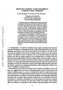
Figure Legend Figure 1: Results for the simulation study with Q-type moves. Figure (1a) shows the
conditional percentiles of the weights. The parallel-ness of these quantile locations is predicted by theory in Section 5 and is the basis for strati ed truncation estimate. Figure (1b) is the histogram of the log-weights and Figure (1c) is the q-q plot of the upper tail of the log-weights versus exp(1). Figure (1d) shows the convergence of the importance sampler estimates, even when the weight has in nite mean.
Figure 2: The corresponding results for the R-type moves. Figure 3: The expected absolute value of the spontaneous magnetization (de ned as P E j i �ij=d , where d is the lattice size) is plotted against various temperature K in Figure 2
4a for 2D Ising model with lattices of size 322 , 642 , 1282 , and in nite. The smooth curve in Figure 4a corresponds to the theoretical in nite lattice result. Figure 4b shows the plot of the conditional quantiles of the weights at 5 typical magnetization values. Our theory in Section 5 predicts that the lines connecting the same quantiles should be approximately parallel.
25
Figure 1
(b)
2000 4000 6000 8000 10000 12000 14000
(a)
6
• •
5
• •
4 •
0.975 •
•
0.95 •
•
•
0.90 •
1
•
•
•
• •
•
0.80 • 0.70 • 1
• •
•
•
•
0
3
percentile of log-weight
0.99 • •
•
2
•
• •
2
3
4
5
0
2
state
4
4
10
•
6
8
0.4 0.3 0.2
• •
• • •
0.1
standardized error
0.5
0.6
• •• • •• •• • ••• •••• •••••• •• •••• ••••••••• • • • • ••••••• •••••• ••• ••••• ••••••• ••• • • • • •• ••••• •••• ••••• ••••• ••••• ••••• • • • •• ••••• ••••• •••• ••••••• ••••• ••••• • • • ••••• •••• •••••••• ••••• 2
8
(d)
• • •
10
5
exp(1)
• •
•
• •
•
•
10
15
20
log-iteration
26
• • • • • • •
•
0.0
6 4 2
log weight of state 3
8
10
(c)
0
6
histogram of log-weight of state 3
25
Figure 2
(a)
(b)
4000
12
• • • •
•
•
•
•
3000
• 0.975
•
•
•
2000
0.95
•
• • •
0.90
•
0.80
• •
•
6
•
•
•
0.70
•
1
1000
•
•
•
2
3
4
0
10
•
•
8
percentile of log-weight
0.99
•
5
0
5
state
4
6
8
•
•
•
•
•
0.3
0.4
•
• •
0.2
standardized error
0.5
0.6
•
• • •
•
5
exp(1)
10
• • •
• 10
•
•
•
•
0.1
12 10 8 6
log weight of state 3
14
16
• • ••• • •• •••• • ••• • • • •• ••• •••••••• ••• •• • • • • •••• •••• ••••• ••• ••• • • •• •••• ••• ••• ••• ••• • •• ••• ••• ••• ••• • • • ••• ••• ••• ••• 2
15
(d)
0.7
(c)
0
10
histogram of log-weight of state 3
15
•
• •
20
log-iteration
27
•
25
Figure 3 (a)
0.8
theoretical value 128 by 128 grids 64 by 64 grids 32 by 32 grids
o o o
o
o o o • o o • o
•
•
•
0.6
o
0.4
•
0.2
o
• o • •
•
o o o o o
o
o
0.0
|M|
• o
0.40
0.42
0.44
0.46 K
28
0.48
0.50
Figure 4
12
(b)
• •
10
•
0.99
•
•
•
•
8 0.975
•
0.95
•
•
6
•
• •
• • • •
•
4
• •
0.80
•
•
•
•
0.90
•
•
•
0.70 •
2
percentile of log weight
•
•
0.86
0.87
0.88
0.89 |M|
29
0.90
0.91