IEEE TRANSACTIONS ON MEDICAL IMAGING, VOL. 23, NO. 7, JULY 2004
807
Automatic Identification of Bacterial Types Using Statistical Imaging Methods Sigal Trattner, Hayit Greenspan*, Member, IEEE, Gabi Tepper, and Shimon Abboud
Abstract—The objective of the current study is to develop an automatic tool to identify microbiological data types using computervision and statistical modeling techniques. Bacteriophage (phage) typing methods are used to identify and extract representative profiles of bacterial types out of species such as the Staphylococcus aureus. Current systems rely on the subjective reading of profiles by a human expert. This process is time-consuming and prone to errors, especially as technology is enabling the increase in the number of phages used for typing. The statistical methodology presented in this work, provides for an automated, objective and robust analysis of visual data, along with the ability to cope with increasing data volumes. Index Terms—Bacteria image analysis, phage typing, spot finding, statistical modeling, visual-array data.
I. INTRODUCTION
I
MAGE processing and computer modeling are important tools in most medical imaging domains, and have more recently started to attract the attention of the biological community and to take a growing role in biological imaging applications. Todate, many of the biological and microbiological data analysis entail a substantial amount of human intervention. Manual procedures are based on subjective human interpretation, are prone to large variability between the human experts, are time consuming and are of great cost. Automated tools are, thus, important in achieving objective and repeatable analysis, accurate quantitative measurements as well as the analysis of increasing data volumes. In this paper we combine imaging analysis with statistical modeling tools in a general framework for visual array analysis. We focus on microbiological data, in particular on bacterial type modeling. We start with an introduction to the biological data following which we introduce the general field of visual array analysis. Bacteria are identified as the main cause for disease outbreaks [1]. Defining an effective and preventive treatment involves
Manuscript received January 8, 2004; revised February 15, 2004. The Associate Editor responsible for coordinating the review of this paper and recommending its publication was M. Sonka. Asterisk indicates corresponding author. S. Trattner is with the Department of Biomedical Engineering, Faculty of Engineering, Tel-Aviv University, Tel-Aviv 69978, Israel (e-mail: trattner@ post.tau.ac.il). *H. Greenspan is with the Department of Biomedical Engineering, Faculty of Engineering, Tel-Aviv University, Tel-Aviv 69978, Israel (e-mail:
[email protected]). G. Tepper is with Spring Diagnostics Ltd., Rehovot 76472, Israel, (e-mail:
[email protected]). S. Abboud is with the Department of Biomedical Engineering, Faculty of Engineering, Tel-Aviv University, Tel-Aviv 69978, Israel (e-mail: abboud@ eng.tau.ac.il). Digital Object Identifier 10.1109/TMI.2004.827481
a characterization of the disease outbreak by identifying its pathogens. The identification of pathogens in a bacteria level or bacteria-species level is not satisfactory for epidemiological and clinical concerns, in particular due to increasing bacterial adaptation to human environments including resistance of bacteria to antimicrobial agents. Therefore, a bacterial type diagnosis is required, i.e., the identification of pathogens below the species level [1]–[4]. This yields information for controlling the disease. Subgrouping of bacterial species to types (bacterial types) are used for many important pathogenic bacteria such as the Salmonella and the Staphylococcus aureus (S. aureus). The S. aureus species is a major cause of community-acquired infections as well as farm animals’ diseases such as mastitis of lactating cows [1], [2], [5], [6]. It is particularly important due to the bacteria tendency to develop resistance to antibiotics. Phage typing is a method for determining the species reactivity to a set of selected bacteriophages (phages) [1], hence, to define its type. A phage is a bacterial virus activated by specific bacterial surface constituents of the checked species. The phage receptor binds to a matching bacterial surface component, invades and multiplies in the bacterial host. When a phage infects a layer of bacterial cells, a zone of lysis produces a plaque, viewed as a clear area in the bacterial lawn, such as the full circles (spots) in Fig. 1. These represent positive reactions to different phages. When the phage receptor does not recognize any of the tested bacterial surface constituents, no plaque is formed and it is defined as a negative reaction. In this case, no surface change is visible. The molecules from each phage strain, involved in interactions such as described, are specific for bacterial types and are known to correlate with important epidemiological factors. The set of phages active against a culture of bacteria isolates forms a unique profile specific for each bacterial type. We term this profile the “phage profile.” Recently, a new approach for phage production and phage typing has been developed by Spring Diagnostics [6]–[8]. The production technology enables a much larger quantity of typing phages (mutants) than the present international sets that are used. A phage typing experiment consists of placing the phages on a monolayer of pure bacterial culture by using a printhead. Each of the pins, in an array order, places a different phage (Fig. 1). Phage typing is performed manually. The distinction between positive and negative reactions is defined by parameters of brightness level, size of reaction, and graininess level. Significant expertise to perform and to interpret the results still yields ambiguous results of typing information [3]. Large variability exists in the decision making process and the analysis is time-consuming.
0278-0062/04$20.00 © 2004 IEEE
808
IEEE TRANSACTIONS ON MEDICAL IMAGING, VOL. 23, NO. 7, JULY 2004
Fig. 1. Examples of visual arrays of phage reactions. Image variability and irregularities within the image database are shown: Differences in contrast and dynamic range of grayscale; irregular spot shape and size; nonuniform background and added contamination.
A. Visual Array Analysis: Spot Finding & Spot Categorization The task of identifying a bacterial type phage profile belongs to the general task of image array analysis. Image array analysis includes a spot finding task, to determine the localization of spots, and a spot analysis task. We address the task of spot finding as well as spot categorization (labeling spots into positive and negative reactions) and phage profile extraction.1 To the best of our knowledge, no previous work has been done on automatic spot analysis for phage typing. Related work on spot finding has been described for microarrays and macroarrays, both on rigid slides and on flexible membranes. Many works on spot finding are found in the domain of cDNA microarray data analysis, where the goal is to identify the locations and extents of labeled DNA spots in a scanned microarray image [9], [10]. An accurate localization of spots in visual array data is important, as location errors may propagate to all subsequent analysis. The spot finder must be robust to substantial uncertainties in spot size and position as well as to diffuse image noise and discrete image artifacts arising from airborne particles or nonuniform washing of the array surface. The need to overcome position and size variations while dealing with image noise and artifacts is a principle source of complexity in solving the spot finding problem. Two closely linked objectives, image segmentation and grid positioning, are often described in the spot finding task. It is common practice to separate the signal from the background on the basis of a preliminary grid overlay [e.g., [9]–[11]]. The grid partitions the image plane into windows, rectangular units uniformly spaced in an array overlayed on the image plane, such that each window contains a single reaction (spot). The windows are analyzed locally, each one separated into a spot region and a background region. Grid placement is commonly achieved with human intervention. The grid configuration definition, expected size and shape of a spot, size of mask to contain all spots [11]–[18] or manual tracing over the image [9], are all predetermined inputs by the human expert. A different approach for grid placement, which is based on a Markov Random Field model of a deformable lattice [19], 1A preliminary report of this work was presented at the SPIE International Symposium on Medical Imaging, San Diego, CA, Feb 2003.
does not require user intervention; yet, computationally this approach seems to be complex. A segmentation stage follows the gridding procedure. Various methods have been used to segment each window. Segmentation algorithms include fixed circle segmentation [20], adaptive circle segmentation [12], [13], adaptive shape segmentation [14], [15] using watershed algorithms [21], and seeded region growing [22] as well as histogram-based segmentation [16]–[18]. Human intervention is important in most of the above-mentioned methods. Manual input may consist of roughly circling the spot regions, a priori setting the grid partitions and in determining parameter settings, such as intensity thresholds, the shape and size of spots in the window, etc. The framework proposed in this paper is different from existing array analysis works in several ways. First, a strong focus of the current work is on spot categorization and analysis, which was not previously done in the domain of phage typing. The spot finding task is defined as a dual stage process that involves global image segmentation into signal versus background regions via unsupervised clustering, followed by a gridding procedure that provides localization of the individual spots. Note that global processing leads to localized processing, as opposed to most works in the field in which the gridding process is a crucial first step of the system. Following the spot finding stage, statistical analysis of spot region characteristics enables probabilistic categorization of the spot reactions. A final processing step transitions from the spot categorization to phage profiling per baterial type. Minimal amount of human interaction is included throughout. The paper is organized as follows: Input data characteristics are presented in Section II. The methodology involving computer-vision and statistical modeling is presented in Section III. Experimental results on the S. aureus are shown in Section IV. A discussion of the results is conducted in Section V. II. DATA CHARACTERISTICS Gray-level images of phage typing arrays are the visual input to the proposed system. The images are scanned using a UMAX scanner, Powerlook2 model, with a transparency adaptor. Each image is of size 532 532 pixels. An example of scanned images is presented in Fig. 1. The Petri-dishes seen in the images
TRATTNER et al.: AUTOMATIC IDENTIFICATION OF BACTERIAL TYPES USING STATISTICAL IMAGING METHODS
809
Fig. 2. A plot of signal (reaction) and background intensity distributions of one image group (40 images).
contain a surface of S. aureus species. Reactions to 60 different phages are present on the surface of the dish. The reactions are organized in a fixed array and known order. An image group contains a set of images. A given database consists of image groups, each group representing a particular S. aureus bacterial type. A significant variability between the scanned images and irregularities in each image exist within a given database. The large variability is exemplified in Fig. 1. Image contrast and dynamic range are considerably different across the image group. Reaction shapes and sizes are irregular, both within an image as well as across the images. Reactions are not positioned in a uniform layout. Finally, the background, i.e., the dish surface, also exhibits nonuniformity due to inevitable differences in experimental conditions, and variability in the pigmentation of bacterial isolates. The large image variability may be due to the following considerations: • Environmental parameters that are related to the experimental setup, including temperature, medium, nutrient concentrations, and quantity. Minor deviations in the accuracy of these parameters may cause significant changes in the species surface and the reactions characteristics [23]. • Mechanical hardware limitations of phage printing, such as the vibration of the pins within the printhead, may cause inaccurate location of spots. Phage imprinting also affects the reaction development and may cause the appearance of elementary plaques (seen as small bright particles). • Minor contamination with environmental bacteria that is seen as dark particles. • Differences among bacteria variants in growth rate and pigmentations affect the intensity of the reactions. • Nonoptimal illumination may lead to changes of the background intensity within an image and across the images in the database. The large variability of the intensity distributions in positive reaction regions (signal) and in background regions, within a single image group, is illustrated in Fig. 2. The brightness levels
Fig. 3. Statistical analysis framework: from the visual array to the phage profile representing a bacterial type. The input consists of a single image group. Each image is preprocessed, segmented and has a grid positioned on it, as part of the spot finding task. The next stages process the entire image group. They include spot categorization and phage profiling.
(intensity) of positive reaction regions are seen to overlap brightness levels of background regions in the different images. The large variability in the image characteristics makes the interpretation of reactions and their classification, a complex task. In this paper, we do not deal with the environmental or mechanical limitations of the laboratory experimental process or the image acquisition process. The focus is on improving the reaction categorization accuracy by achieving invariance to the obstacles mentioned above. III. METHODS The proposed framework is presented in Fig. 3. Visual array data is processed via two key processing stages: a segmentation stage and a follow-up categorization stage. Statistical modeling via Gaussian mixture models (GMMs) and expectation-maximization (EM) learning are utilized in both stages of analysis. The objective of the segmentation phase is to extract a probabilistic separation of the data, per image, into two main regions: the signal (phage reaction) region; namely, the spot, and the background region. An alignment of a grid onto each image is enabled based on the achieved segmentation. Following the segmentation phase, spots are analyzed further. A set of feature vectors extracted per image group is analyzed statistically for modeling positive and negative reactions. Using the learned
810
IEEE TRANSACTIONS ON MEDICAL IMAGING, VOL. 23, NO. 7, JULY 2004
model a categorization of each spot into the positive and negative clusters is enabled. A transition is made to phage profiling and the final output is a probabilistic signature of phage-reaction profile (phage profile) per image group. The processing stages are described in detail in the following subsections. A. Segmentation Stage: Signal Versus Background In order to facilitate the segmentation process, an initial preprocessing step is used to remove artifacts and improve the image contrast and dynamic range. The preprocessing stage consists of an initial high-pass filtering. The high-pass filter helps to remove a low-frequency signal observed experimentally to be an undesired component of the background. In addition, we find that emphasizing the high frequencies augments the signal (reaction) regions. A normalization step follows which extends the dynamic range. Additional details are given in Appendix A. The segmentation stage is defined as an unsupervised clustering task. The segmentation is performed globally, as a one-time process on the entire image plane (rather than window by window). The only a priori assumption made in the process is the existence of two main clusters to be learned. The choice of two clusters is biologically and physically driven, as we expect a Gaussian distribution of the signal intensity values and a Gaussian distribution of the background intensities (see Fig. 2). In the following section, we introduce the GMM and the related EM algorithm, following which we describe the unsupervised clustering scheme for segmentation. An experimental comparison to different segmentation approaches is described in Appendix C. 1) Data Representation via GMM: The GMM is a semiparametric approach to density estimation [24], based on utilizing a model that best fits the input data. In modeling image data, an initial transition is made from the raw pixel input to a selected feature space. Following the feature extraction stage each pixel is represented by a feature vector and the image as a whole is represented by a collection of feature vectors. The pixels are then grouped into homogenous regions by grouping the feature vectors in the selected feature space. The underlying assumption is that a mixture of Gaussians generates the image features’ distribution. Note that although image pixels are placed on a regular (uniform) grid, this fact is not relevant to the probabilistic clustering model in which the posterior of a cluster given a pixel value is of interest. In general, a pixel is more likely to belong to a certain cluster if it is located near the cluster centroid. This observation implies a unimodal distribution of pixel positions within a cluster. A natural choice for a unimodal distribution within a GMM framework is a Gaussian distribution. The EM algorithm [24], [25] is used to determine the maximum-likelihood (ML) parameters of a mixture of Gaussians in the feature space. The image is then modeled as a Gaussian mixture distribution in the feature space. The distribution of a random variable is a mixture of Gaussians if its density function is
(1)
such that the parameter set
consists of
where is the prior probability for Gaussian , and , are the mean vector and covariance matrix of Gaussian , respectively. the maximum likeGiven a set of feature vectors lihood (ML) estimation of is (2) The EM algorithm is an iterative method to obtain the parameter set increasing the likelihood function in each iteration. The likelihood function is based on samples that are independent and identically distributed (3) Given the current estimation of the parameter set , an iteration of the EM algorithm re-estimates the parameter set according to the following two steps. • Expectation Step: Estimation of the probability of sample to belong to cluster
(4) • Maximization Step: Estimation of the new parameter set based on the updated probabilities
(5)
Using EM, the parameters representing the Gaussian mixture are found. Initializing mixture model parameters of the EM algorithm is done using the K-means algorithm [24], [25]. The update scheme defined above allows for full covariance matrices; variants include restricting the covariance to be diagonal or scalar matrix. The updating process is repeated until the log-likelihood is increased by less than 1% from one iteration to the next. It is common knowledge that the number of mixture components, , is of great importance in the accurate representation of the data. Ideally, represents the value that best suits the natural number of groups present in the data. The number of a priori assumed clusters can be defined appropriately by the user or
TRATTNER et al.: AUTOMATIC IDENTIFICATION OF BACTERIAL TYPES USING STATISTICAL IMAGING METHODS
811
found via automated techniques, such as the minimum description length principle [26]. In this paper, the number of clusters is predefined based on the data at hand, as found appropriate for the S. aureus bacteria. 2) Probabilistic Segmentation: The segmentation process is based on clustering of the pixel intensity values per image. The image is represented by a mixture of two Gaussians ( ), one Gaussian represents the image signal values, the other represents the image background intensity distribution. The choice of is based on the a priori analysis of the data at hand (see Fig. 2). Once the model is learned, the probabilistic affiliation of each image pixel with each of the Gaussians in the model ) can be computed. From Bayes rule ( (6) Each pixel (feature vector) of the original image, affiliated with the most probable Gaussian cluster
, is then
(7)
B. Grid Positioning: From the Image Plane to Image Spots The result of the segmentation phase is a binary image in which an estimate of the signal region is given. In the next phase of processing we transition from the global image signal to localized reactions, or spots. Extracting local areas of interest in an input image is accomplished by partitioning the data into windows via a grid. In this paper, we position the grid automatically based on the segmentation results. The grid-positioning algorithm is as follows: Starting with its original state, each binary (segmented) image is rotated in intervals of 1 between 10 and 10 . For each angle of rotation , a projection (sum) over the axis and the axis is computed. Thus, we get two projection funcand for the axis and the axis, respectively tions, (Fig. 4). The angle by which the image has to be de-rotated is determined by the angle for which a maximum projection value is found (8) The image location for which the maximum projection value is found serves as an anchor point from which the grid is defined (9) where and are the two projection functions for the axis and the axis, respectively, of the image de-rotated by . The set of maximal-strength signal value locations is extracted from the and profiles and an average grid interval is defined. The grid is defined around the anchor point, in equal intervals as learned from the data (i.e., the average grid interval). Utilizing the grid, spot finding is accomplished; A transition can be made to local image analysis and further spot processing, as described next.
Fig. 4. Grid placement is determined using projections in the x and y directions.
C. Spot Analysis and Categorization The goal of the spot analysis stage is to categorize the spot as a positive or negative reaction. A hard threshold on the intensity values is not sufficient for the categorization task, due to the large variability of the raw data (see Fig. 1). A reaction is defined as positive, when there are a sufficient number of pixels of high-intensity present (to be determined), and a circular structure is evident. A transition is, thus, made from the raw pixels to a feature space that accommodates the signal strength and morphology criteria. The labeling task becomes a clustering task within the selected feature space. The following features are extracted from each spot. 1) Normalized area (NA): The area of a spot, , is the sum of pixels that comprise the spot, i.e., overall signal contained in a window. This sum is normalized by the average spot size within the image. For the average, only spots with an area above a certain threshold, , are considered (10) with the threshold value empirically set to 200. The normalization factor is important in order to achieve invariance to the variability in the positive reaction area across the images in the dataset. The NA feature is, therefore, an estimate of the relative size of a reaction per spot. 2) Shape Index (SI): (11) where is the area of signal and is the perimeter of the signal. This feature is used in the literature as a measure of circularity [27]. The perimeter is computed by summing up edge pixels per spot. We use the SI as a measure of shape and graininess. High values of SI represent spots with higher circularity and less graininess. Prior to the SI feature extraction, the spots are smoothed using the morphological operator of closing [27] with a disk structure element of radius one (treated are only those
812
IEEE TRANSACTIONS ON MEDICAL IMAGING, VOL. 23, NO. 7, JULY 2004
Fig. 5. Transition from spots (per image) to a phage representation.
spots of area greater than the size threshold, ). The purpose of smoothing is to compensate for spots’ graininess due to experimental artifacts and/or due to low-contrast conditions. The smoothing step helps to fill in holes that were created by the extraction of dark particles during the segmentation process. Additional details regarding the smoothing process can be found in Appendix B. , ( ) are exFeature vectors, , across all the images in a tracted from all spots, given image group. Clustering of the features is pursued using ) to sepaGMM and EM. A two-cluster partition is used ( rate the space into the positive and negative reaction categories. The choice of a two class partitioning is motivated from the biological categorization of the spots into two reaction groups. ) may be appropriate Using more than two clusters ( in cases in which we are interested in defining intermediate reaction types. In the presented task, using a larger would have resulted in a larger set of clusters and an additional decision step would be necessary to allocate the clusters into the positive-reaction clusters and the negative-reaction clusters. Utilizing the learned GMM model, the probabilistic labeling of each spot is enabled [see (6)]. The affiliation of each spot to the most probable Gaussian cluster [see (7)] produces image spot categorization. D. From Spots to Phage Profiling
Fig. 6. Example of image segmentation: (a) The original image (left). Corresponding intensity histogram (right); (b) Preprocessing the input image; (c) Segmented image (left). GMM learned via unsupervised clustering (k = 2) of the image pixels (right).
A standard-deviation measure is computed over the spot probabilities to estimate the variability in the spot reactions within the image group. The phage profile is taken as a collection of phage labels along with the average probabilities per phage, extracted in a predefined order across the image array. A profile thresholding step may be used such that the final reduced-size phage profile contains only those phages for which a high-probability decision was made. The phage profile serves as a fingerprint of a bacterial type of the image group checked. IV. EXPERIMENTAL RESULTS
A final transition is made from the level of spot categorization to the level of phage profiling per bacterial type, as illustrated in Fig. 5. Each phage ( ) is probabilistically affiliated with the positive and negative reaction categories ( ), by averaging across the corresponding spot probabilities (12) with the averaging performed over the spots, , , related to the same phage, , for all images in the image group. A hard decision step is taken to finalize the labeling process. The phage label is determined by the higher average probability of the two (13)
The proposed framework automatically analyzes visual array data, and provides information about the spot locations and categorizations, as well as phage profiles. In this section we present experimental results for both spot and phage level analysis. The results demonstrate the tasks of spot finding (Section IV-A) and spot categorization (Section IV-B), and the analysis of phage profiles as representatives of image groups and bacterial types (Section IV-C). As there is no standard means of validation for all the above tasks, validation methods based on the available ground-truth, will be defined per task. Two datasets are used. Dataset I consists of 4 image groups, where each image group is taken from a different farm. Each farm corresponds to a particular bacterial type. Three image groups (#1, #2, and #4) consist of 40 images. Group #3 contains 260 images. Dataset II consists of 2 image groups, con-
TRATTNER et al.: AUTOMATIC IDENTIFICATION OF BACTERIAL TYPES USING STATISTICAL IMAGING METHODS
813
Fig. 7. Examples for segmentation, gridding and smoothing: (a) Original images. (b) Segmented images. (c) Images overlayed with grid (de-rotated). (d) Smoothed images.
taining 328 and 72 images. The image groups in dataset II have been verified as two different bacterial types using a leading DNA-based typing method (the pulsed field gel electrophoresis (PFGE) method [3], [23]). In both dataset I and dataset II, a (36) phages is analyzed per Petri-dish central subarray of image, to avoid edge effects. Four Petri-dishes are input at a ) phages are considered in a time, thus, a total of 144 ( phage profile. A. Segmentation Results: Spot Finding Fig. 6 presents an example of the segmentation process. In Fig. 6(a), the original image is shown (left) with its corresponding intensity histogram (right). The low contrast of the image is evident in the image plane as well as in the gray-level distribution. The preprocessing stage alters the histogram to include two intensity peaks representing signal and background regions and enhances the contrast as shown in Fig. 6(b). Using the processed image data a GMM is learned [Fig. 6(c) right]. Each pixel of the original image is next affiliated with the most probable Gaussian [see (7)] to provide the final segmentation
Fig. 8. The learned GMM for the input data. The two modes represent positive and negative reactions.
map, as presented in Fig. 6(c) left. Note that pixels that are affiliated with the “signal” Gaussian are displayed in white, while pixels that are affiliated with the “background” Gaussian are displayed in black. The separation between the signal and
814
Fig. 9.
IEEE TRANSACTIONS ON MEDICAL IMAGING, VOL. 23, NO. 7, JULY 2004
Examples of the algorithm spot categorization along with corresponding probabilities.
background regions is evident. Also evident is the graininess within the signal regions. This graininess may be the result of the image low contrast and artifacts contaminating the input image [see Fig. 6(a)]. The dark-particle noise evident in Fig. 6(b) is removed in the segmentation process while the bright noise artifacts are interpreted as signal. Additional segmentation results, along with gridding and smoothing are shown in Fig. 7. In Fig. 7(a), the original images are shown. The variability of contrast and dynamic range across the images is evident, as well as the background variability within the images. The segmented images are shown in Fig. 7(b) following de-rotation. The graininess present in the segmented images is due both to the low-contrast input (as in image #1) as well as to biological reactions (as in image #2). The corresponding grid overlay is shown in Fig. 7(c). Smoothed segmented images (used in the follow-up feature extraction stage) are presented in Fig. 7(d). The effect of smoothing on the algorithm performance, using structure elements of differing sizes, is discussed in Appendix B. The global GMM approach is used for the segmentation task. We have found this approach to give satisfactory results. A comparison of the global GMM to other segmentation algorithms is given in Appendix C. B. Results of Modeling in Feature Space: Spot Categorization Fig. 8 presents an example of a GMM learned from all feature-vector samples [SI, NA] for a particular image group (see Section III-C). A clear separation between the two major modes is evident, with one cluster (Gaussian) representing positive reactions and the second cluster representing the negative reactions. The spread of each cluster defines the variance in each group of reactions.
TABLE I CORRELATION AND STATISTICAL RESULTS OF EXPERT-BASED CATEGORIZATION VERSUS AUTOMATIC CATEGORIZATION
Spot categorization is achieved by computing the probabilistic spot affiliation to each of the Gaussians of the learned GMM, and then determining the most probable Gaussian cluster [(6) and (7)]. Fig. 9 presents examples of two images with spot categorization. The reaction category is indicated ), along with its probability. A correlation is evident be( tween the numerical probabilities and human perception. Spots that are perceptually very clearly categorized (into positive or negative reactions) are supported with higher probabilities than spots for which the reaction category is visually questionable. Spot categorization results were validated with human-expert labeling as ground-truth. Automatic spot categorization results from dataset II were compared with supervised categorization of 7992 spots, which were ascribed a label of positive and negative reactions by an expert. Results are given in Table I. The algorithm achieved a correlation of 95% with the supervised categorization. A 98% correlation was achieved with the supervised positive categorization (sensitivity) and an 89% correlation was achieved with the supervised negative categorization
TRATTNER et al.: AUTOMATIC IDENTIFICATION OF BACTERIAL TYPES USING STATISTICAL IMAGING METHODS
815
TABLE II AN EXAMPLE OF A PHAGE PROFILE (27 OUT OF 144 PHAGES). EACH PHAGE IS IDENTIFIED BY A SERIAL NUMBER AND IS AFFILIATED WITH A REACTION TYPE ( OR ). THE AVERAGE PROBABILITY FOR THE REACTION TYPE IS SHOWN, ALONG WITH THE CORRESPONDING STANDARD DEVIATION
+ 0
TABLE III A PROFILE FOLLOWING REACTION THRESHOLD. IN THIS EXAMPLE AN 80% THRESHOLD IS USED ON THE PROFILE IN TABLE II. PHAGE LOCATIONS IN WHICH THE CATEGORIZATION PROBABILITY WAS LOWER THAN 80% ARE NULLED OUT (“X”)
Fig. 11. Two images from two image subgroups for which profiles are displayed in Table IV Phage number 19 is highlighted. A clear distinction in the reaction is evident. Fig. 10. A histogram of the number of identically labeled spots categorization (ILS) in spot profile pairs being compared.
(specificity). The positive predictive value, i.e., the probability that the spot reaction is manually categorized as positive when the automatic categorization is positive, is 98%. The negative predictive value is 96%. In a second validation step, the goal is to explore if unsupervised clustering of the spot reactions may find image groups corresponding to bacteria-types. Spot categorized images are used to form a spot profile per image input (note that a spot profile characterizes a single image whereas a phage profile characterizes an image group). Pairs of spot profiles are compared by counting the number of identically labeled spots (ILS). A histogram is generated consisting of ILS values. Clusters in the histogram indicate image similarities and can be used to suggest potential image groups in the datasets. A validation strategy in this scenario is to compare the learned image groups to the a priori defined image groups in the datasets. Fig. 10 shows a histogram of spot profiles that are extracted from all the images in dataset II. Two main clusters are seen. The smaller ILS values correspond to pairs of profiles that are distinct while the larger ILS values correspond with similar pairs of profiles. A comparison between the automatically extracted clusters to the predetermined image groups, indicates a complete match.
C. Phage Profiling and Analysis An example of a phage profile (27 out of 144 phages) is shown in Table II [(12) and (13)]. The categorization of each phage is given in the second row. The corresponding average , and standard deviation ( ) are listed in the probability, third and fourth rows, respectively. A high average probability indicates a similar (and strong) spot reaction in the particular image location, across the images in the image group. For example, consider phage #7 in Table II. The category is the negais 100 with a of 0. We can conclude tive category ( ), from this that all spots in the image group have a negative reaction at 100% probability. A low average probability indicates either that the spot reactions (per phage) are not similar, which value, or that for each labeled will be evident in a large spot, the affiliation probability is low [(6) and (7)]. Phage #24 of 50% and a large . in Table II, for example, has a The spot reactions for this phage are in fact split, with half of the spots having a large probability for the positive reaction and half of the spots having a large probability for the negative reaction. An example of profile thresholding using a threshold value of 80% is shown in Table III. Here, symbolizes phages that are not considered as part of the bacteria signature, or in further processing. The threshold step reduces the number of phages to 116 phages (out of 144). Depending on the number and biological significance of the phage set that is nulled out, the expert
816
IEEE TRANSACTIONS ON MEDICAL IMAGING, VOL. 23, NO. 7, JULY 2004
TABLE IV AN EXAMPLE OF A PHAGE PROFILE (27 OUT OF 144 PHAGES) FOR SEVEN IMAGE-SUBGROUPS TAKEN FROM A SINGLE IMAGE GROUP. PHAGE REACTIONS ARE SHOWN IN THE TOP ROWS WITH THE AVERAGE PROBABILITIES LISTED IN THE BOTTOM ROWS. SIMILAR REACTIONS ACROSS THE SEVEN PROFILES ARE INDICATED IN GRAY. NONUNIFORM PHAGE REACTIONS (SUCH AS IN PHAGES 17, 19, 23, and 24) HAVE CORRESPONDING LOW AVERAGE PROBABILITIES.
Fig. 12. Image examples from each of the four image groups (Database I). Differences are visually evident between groups #1, #3 and #4. Similarity is present between groups #2 and #3.
may consider the significance of the profile signature and if it sufficiently represents the bacterial type. We utilize the phage profiles for bacterial type diagnosis. It is not the goal of the current work to label the various types. Rather, the focus is on evaluating the phage profiles extracted, as a basis for analyzing similarities and differences of bacterial types. An assumption in this paper that serves as the groundtruth is that an image group corresponds with a particular bacterial type. In validating the phage profiles generated by the proposed system, profiles that are extracted from image groups of a similar bacterial type are expected to have a similar signature, while phage profiles that are extracted from image groups of different bacterial types, are expected to show large profile variations. The comparison between phage profiles is measured as the percentage of similar categorization (PSC) between the phages. In the following experiments, we investigate phage profiles and the PSC value in both datasets. Dataset I: A given image group of 260 images is divided into seven subgroups of images. A phage profile is generated for each image subgroup. Table IV presents the seven phage profiles generated (27 out of 144 phages are listed). The top part of the table indicates the reaction type ( or ) per phage. The bottom
part of the table contains the average probabilities of the reactions, respectively. When all 144 phages are compared, i.e., no thresholding is done, the PSC value across the seven subgroups is 78%. An example of a phage for which the reaction category is not consistent is shown in Fig. 11. Two images from two of the image subgroups are shown, with a window overlayed on phage #19. The evident visual differences in the reaction appearance provide an insight into the difficulty of categorizing this particular phage. Table IV indicates low average probabilities along with nonuniform reactions for this phage. Profile thresholding with an average probability threshold value of 80%, results in a reduced size profile of 96 phages. Within this more compact phage profile set, the PSC is 100%, i.e., a full similarity is achieved across the seven profiles. Fig. 12 shows representative images from the four image groups. Visual inspection of the images as well as the phage profiles indicates a difference between groups #1, #3, and #4, with a similarity between groups #2 and #3. Fig. 13(a) displays corresponding PSC values. The similarity percentage is plotted versus the percentage of profile thresholding. Three curves are shown, each representing PSC values for a particular pair of image groups. The curve representing groups #2 and
TRATTNER et al.: AUTOMATIC IDENTIFICATION OF BACTERIAL TYPES USING STATISTICAL IMAGING METHODS
817
TABLE V PROFILES FROM FOUR IMAGE-GROUPS (NO THRESHOLDING).
Dataset II: A similar profile analysis is conducted for the two image groups of the second dataset, as shown in Fig. 13(b). Two curves are shown. One represents two subgroups within image group 1. The second curve is a comparison of profiles of image group 1 and image group 2. A clear distinction is evident. Using the full profiles (no thresholding), a 40% similarity is present between the two image groups. A close to 100% similarity is seen between the two subgroups. Thresholding the profiles augments the difference between the group signatures, validating the hypothesis that two distinct bacterial types are present. V. CONCLUSIONS AND DISCUSSION
Fig. 13. The PSC in different pairs of image groups versus the percentage of profile thresholding. (a) Dataset I; (b) Dataset II.
#3 has a high percentage of similarity of above 90% without any thresholding, and an increased value of 100% following profile thresholding. These high similarity values match with the visual similarity seen between the two groups. Table V presents the phage profiles generated for the four different image groups of Dataset I. Fig. 13(a) shows a similarity percentage of less than 60%, without thresholding, in the comparison between groups #1 and #3, and groups #4 and #3. The distinct groups remain mostly around the 60% and 70% range throughout. From these results, it may be concluded that different bacterial types are present in groups #1, #3 and #4. The same type is most likely present in groups #2 and #3.
This paper presents an automated framework for translating large sets of visual array information into probabilistic phage profiles representing bacterial types. In many biological applications the amount of data is constantly increasing and the need to shift from manual work to an automated means is of importance for efficient and accurate research and production. The goal of image array analysis is to achieve spot analysis using advanced computer vision algorithms, with no or minimal need for human intervention. Such systems would greatly reduce the human effort, minimize the potential for human error and offer data consistency. In this paper, visual array data was segmented and categorized utilizing statistical imaging methods. GMM and EM learning were used in both the segmentation and the categorization stages of the framework. The output of the system is a probabilistic phage profile representing the input image group. Several key points distinguish the presented framework from existing works on visual array processing. In most current systems, the human expert is an important part of the analysis procedure, introducing and modifying a variety of thresholds for the task, and/or placing the grid manually to begin with. In the current work, the segmentation and categorization algorithms are based on unsupervised clustering, thus, are adaptive to the data at hand and require minimal human intervention. The gridding process, which transitions the global analysis to a localized, spot-based analysis, is enabled automatically as a result of the segmentation process. In the spot categorization task, morphology features are used, in addition to the commonly used intensity features. This paper introduces, defines and evaluates the use of spot analysis for probabilistic phage profiling. An important consideration in evaluating the proposed system is its ability to cope with the variability within the scanned image sets and irregularities inherent within the visual array database. Figs. 2 and 7 demonstrate the differences in contrast, spot size and nonuniformity of the background found
818
in the data. Thresholding techniques that use user-defined thresholds, are very limited in their capabilities to segment the data into signal and background regions, as well as to categorize the signal data into positive and negative reactions. Such techniques require that the thresholds be manually adapted, several times per image. In this study, automatic adaptation is enabled via statistical modeling of the data per image, both in the segmentation as well as the categorization tasks. Fig. 8 shows the clustering achieved using a GMM in the feature space selected for the current work. The evident separation of the two clusters validates the features used. The combination of the NA and SI features was selected following experimentations with many other possible features, such as the median, total intensity, entropy, ratios of longest axis, and more. The two clear modes present in Fig. 8 indicate the robustness to factors of variability within the data. Invariance to size is well demonstrated in Fig. 9, where both small and big reactions were identified as positive reactions with high probabilities. The categorization was not affected by the different contrast. Defining good validation strategies proves to be a challenge in many medical imaging domains. Several criteria were used in evaluating the presented framework. Supervised validation was used in the spot categorization task, with a comparison to human expert labeling. Unsupervised clusters were found within the spot profiles, later to be compared to predefined image groups that serve as the phage profile ground truth. Two different signature extraction methodologies were used in defining the image groups: phage-typing (manual) of dataset I and both phagetyping and PFGE of dataset II. On the phage level, supervised validation is used, with the automated profile extraction results compared to the predefined image groups. Spot analysis experiments and results are described in Section IV-B. Clustering of spot profiles achieved high correlation (100%) with the predetermined groups. A strong correlation, of 95%, was found with the human expert labeling (Table I). It is important to note that manual-based ground truth is, in itself, prone to errors. In many instances, the decision of the algorithm may provide more accurate estimates than the human expert. An example is illustrated in Fig. 14. Both marked spots are categorized as positive by the algorithm, whereas the expert marked the two spots differently, biased from the neighboring spots’ signals. Many similar cases to Fig. 14 were found, which may explain the 89% specificity. An important objective of the work is the ability to identify similarity and distinction amongst phage profiles within and across image groups. Examples of phage profiles were shown in Section IV-C. Fig. 13 shows the percentage of similar phage categorization, in different pairs of image groups. In both dataset I (a) and dataset II (b), the phage profiles indicate similarity and differences amongst image groups, in correspondence with the given ground-truth. For example, the two curves of Fig. 13(b) are clearly separated. A distinct behavioral pattern can be seen for the similar phage profiles (two subgroups originating from the same image group) and the different phage profiles (originating from two different image groups). These results are encouraging in that the automated extracted phage profiles seem
IEEE TRANSACTIONS ON MEDICAL IMAGING, VOL. 23, NO. 7, JULY 2004
Fig. 14. Variability in manual categorization. Two spots are marked in squares. One of the spots was manually categorized as positive and the other was manually categorized as negative, in spite of visual similarity. Both spots were determined to be positive by the proposed algorithm.
to be able to validate hypothesis about bacterial types present in a given dataset. The performance of the system is influenced by noise. The magnitude of the noise with respect to the size of the spots (signal) needs to be taken into account. Small noise particles do not influence the categorization but may influence the probabilistic output. Large particles may cause categorization errors. Additional smoothing algorithms may be considered, such as the combination of the GMM modeling with Markov random fields (e.g., [28]). Such a framework may include more specific spatial continuity constraints in the definition of the segmentation task. The experiments so far presented were performed on a limited set of data. In future work we plan to focus on a more exhaustive performance evaluation study. Additional datasets are needed to investigate the same source in a variety of controlled settings (changing the contrast, illumination, noise level, etc). Repeatability across varying images from the same input source is another important experiment that can provide a strong ground-truth mechanism. Our study suggests a generic tool that aids the microbiologist in transforming and supplementing data into useful information for analysis. An objective and consistent processing is provided. The expert can effect the evaluation by determining a (optional) probability threshold, for the compaction of the representative profile into the set of the more probable profile reactions. Probabilistic phage profiling can provide a strong basis for further analysis and bacterial type classification. The methodology presented includes general processing steps that may be applicable regardless of scale: from the micro-array to the macro-array. It should be noted, that in each case, adaptation is needed to the data characteristics, and the required level of accuracy. Related domains include phage therapy, a developing domain related to drug discovery, and the domain of cDNA microarray data analysis.
TRATTNER et al.: AUTOMATIC IDENTIFICATION OF BACTERIAL TYPES USING STATISTICAL IMAGING METHODS
819
APPENDIX A PREPROCESSING Two main components comprise the preprocessing stage: an initial high-pass filtering step and a gray-level normalization step. A. High-Pass Filter High-pass filtering is achieved by subtracting a low-passed version of the original image from the input image. The low-pass filter used is a mean filter [29], in which each pixel is replaced by an equal weighted average of neighborhood pixels (A.1) where and are the input and output images, respectively, is a suitably chosen window of 50 50 pixels is the number of pixels in this determined empirically and window (2500 pixels). B. Normalization A normalization step follows the high-pass filtering, to extend the dynamic range. Each pixel is scaled using the following function: (A.2) where and are the lower (0) and the upper (255) limits, respectively, of gray-level intensities. Parameters and are the input image low and high gray-level intensities, respectively. They are determined per image using the intensity of the 5–10 extreme pixels in the image histogram [30]. APPENDIX B MORPHOLOGICAL OPERATORS FOR SMOOTHING Prior to the SI feature extraction (Section III-C), spots are smoothed using the morphological operator of closing. Suppose that the object and the object are represented as sets in a two-dimensional Euclidean space, then the closing of by is defined as dilation followed by erosion
Fig. 15. Smoothing with different structure elements (discs of different radii) performed on 4 image groups a, b, c, and d with 2772, 2952, 2664, and 1440 spots, respectively. Spot categorization results are compared with manual categorization.
[see (13)]. The importance of the smoothing step is to avoid large perimeter values in grainy spots, which would otherwise give SI values that do not represent the overall circular structure of the spots. The effect of the morphological smoothing and the sensitivity with regard to the structure element size were checked. The algorithm was run with no smoothing and with smoothing using structure elements of different radii. Comparison was made by computing the percentage of correlation of the algorithm spot categorization and manual categorization. Four groups of images with 2772, 2952, 2664, and 1440 spots were checked (database I). The results are shown in Fig. 15. In all cases, smoothing with a radius-1 structure element augments the performance over the nonsmoothed case. This may be the result of the fact that without smoothing, some spots that are grainy with significant signal area may be misclassified as negative spots (with small SI values). The use of other discs of different radii as compared with the radius-1 structure element, does not seem to augment the performance further, rather, in some cases deterioration is seen [as in Fig. 15(b)]. This may be the case due to the increased spot area following the closing operation that may lead to a positive categorization of what should be labeled as negative spots.
(A.3) where is the input image and is called a structure element. Using a structure element of a disk, the closing operation eliminates holes extending into objects in the image. Holes smaller than the structuring element are eliminated. In the case of a grainy object, the closing operator smoothes the object, depending on the relative size of the holes in the object and the structure element. The object overall size grows in an extent depending on the structure element. In this paper, let be the segmented (binary) image (the result of the segmentation process), and represent a structuring element, chosen empirically as a disc with radius one. An initial size-threshold is applied to preserve spots of area greater than the size threshold, , where is empirically set to 200. The smoothed segmentation results are used to extract perimeter
APPENDIX C A COMPARISON ACROSS SEVERAL SEGMENTATION ALGORITHMS The segmentation method implemented in the algorithm is based on the global GMM, i.e., a model that is derived from the entire image. Additional segmentation approaches that were experimented with include a local GMM approach, namely modeling a GMM for each local window separately, and the approach of thresholding the image intensity histogram (at the minimum point between peaks) both globally and locally. We have found the alternative approaches to give less satisfactory results. Fig. 16 shows a segmentation example. Similar spots are marked in the original image (a) and in each of the segmentation results (c)-(f). We shall refer to them as “I” (circle),
820
IEEE TRANSACTIONS ON MEDICAL IMAGING, VOL. 23, NO. 7, JULY 2004
REFERENCES
Fig. 16. Comparison between segmentation results based on different approaches in a single image. (a) Original image. (b) The image histogram after preprocessing; (c) – (f) The segmentation results using the following methods. (c) Global GMM (the presented algorithm). (d) Histogram with a global approach. (e) Histogram with a local approach. (f) GMM with a local approach.
“II” (square), and “III” (rectangle). Spots of high intensity are present in (e): II-III and in (f): I-III. These spots are not compatible with the signal strength as viewed in the original image signal (a):I-III. The localized segmentation approach, for both thresholding (e) and GMM modeling (f) seems to be influenced by local noise and a weak signal in these local windows, augmenting the signal (with no biological significance). Using the global GMM, (c):I-III, a more relevant segmentation is seen. In general, it was observed that the segmentation using the local approach, (e):I-II and (f):I-II, gave stronger signals (the number of pixels defined as signals was higher) as compared with the signals created by the global approaches (c):I-II, (d):I-II. An additional problem with the local approach is the requirement for grid positioning prior to segmentation, which requires user interference. Fig. 16(d) shows the results of global segmentation using thresholding. A weaker signal is extracted (d):I-II, as compared to the equivalent signal in (c). This result may be the case due to an intensity threshold that is higher than the decision boundary in the Gaussian distribution [see Fig. 16(b)].
[1] T. G. Emori and R. P. Gaynes, “An overview of nosocomial infections, including the role of the microbiology laboratory,” Clin. Microbiol. Rev., vol. 6, no. 4, pp. 428–442, 1993. [2] S. Baron, Medical Microbiology, 4th ed. Galveston, TX: Univ. Texas Med. Branch, Sch. Med., 1996. [3] F. C. Tenover, R. D. Arbeit, and R. V. Goering, “How to select and interpret molecular strain typing methods for epidemiological studies of bacterial infections: A review for healthcare epidemiologists,” Infection Contr. Hospital Epidemiol., vol. 18, pp. 426–439, 1997. [4] A. Patrick and D. Grimont, “Taxonomy and classification of bacteria,” in Manual of Clinical Microbiology, 7th ed, P. R. Murray, E. J. Baron, M. A. Pfaller, F. C. Tenover, and R. H. Yolken, Eds. Washington, DC: Amer. Soc. Microbiol., 1999, ch. 14, pp. 249–261. [5] R. D. Arbeit, “Laboratory procedures for the epidemiologic analysis of microorganizm,” in Manual of Clinical Microbiology, 7th ed, P. R. Murray, E. J. Baron, M. A. Pfaller, F. C. Tenover, and R. H. Yolken, Eds. Washington, DC: Amer. Soc. Microbiol., 1999, ch. 7, pp. 116–137. [6] Spring Diagnostics. [Online]. Available: http://www.itek.co.il/spring [7] US PCT Patent application no. PCT/IL00/00 366. [8] G. Teper, G. Ziv, and E. Skutelski, “Flow cytometry analysis of S. aureus – Bacteriophage interactions,” in Proc. 3rd Int. Mastitis Sem., vol. A s-1, 1995, p. 8. [9] Y. H. Yang, M. J. Buckley, S. Dudoit, and T. P. Speed, “Comparison of methods for image analysis on cDNA microarray data,” J. Comp. Graphical Statist., vol. 11, no. 1, pp. 108–136, 2002. [10] G. K. Smyth and Y. H. Yang, “Statistical issues in cDNA microarray data analysis,” in Functional Genomics: Methods and Protocols, M. J. Brownstein and A. B. Khodursky, Eds. Totowa, NJ: Humana, 2003, ser. Methods in Molecular Biology. [11] A. Kuklin, S. Shams, and S. Shah, “High throughput screening of gene expression signatures,” Genetica, vol. 108, pp. 41–46, 2000. [12] J. Buhler, T. Ideker, and D. Haynor, “Dapple: Improved Techniques for Finding Spots on DNA Microarrays,” Univ. Washington CSE, Tech. Rep. UWTR 2000–08–05, 2000. [13] GenePix, Pro Microarray and Array Analysis Software. Axon Instruments Inc. [Online]. Available: http://www.axon.com [14] M. J. Buckley. (2000) Spot User’s Guide, Sydney, Australia. [Online]. Available: http://www.cmis.csiro.au/iap/Spot/spotmanual.htm [15] X. Wang, S. Ghosh, and S. W. Guo, “Quantitative quality control in microarray image processing and data acquisition,” Nucleic Acids Res., vol. 29, no. 15, p. e75, 2001. [16] Y. Chen, E. R. Dougherty, and M. L. Bittner, “Ratio based decisions and the quantitative analysis of cDNA microarray images,” J. Biomed. Optics, vol. 2, pp. 364–374, 1997. [17] QuantArray Analysis Software [Online]. Available: http://lifesciences.perkinelmer.com [18] Scanalytics MicroArray Suite [Online]. Available: http://www.scanalytics.com [19] J. M. Carstensen, “An active lattice model in a Bayesian framework,” J. Comput. Vis. Image Understanding, vol. 63, no. 2, pp. 380–387, 1996. [20] M. B. Eisen. (1999) Sc7anAlyze User Manual. Stanford Univ., Palo Alto, CA. [Online]. Available: http://rana.lbl.gov [21] B. T. M. Roerdink and A. Meijster, “The watershed transform: Definitions, algorithms and parallelization techniques,” Fundamenta Informaticae, vol. 41, pp. 187–228, 2000. [22] R. Adams and L. Bischof, “Seeded region growing,” IEEE Trans. Pattern Anal. Machine Intell., vol. 16, pp. 641–647, June 1999. [23] E. S. Anderson and R. E. O. Williams, “Bacteriophage typing of enteric pathogens and staphylococci and its use in epidemiology,” J. Clin. Pathol., vol. 9, pp. 94–127, 1956. [24] C. M. Bishop, Neural Network for Pattern Recognition. Oxford, U.K.: Clarendon, 1996. [25] H. Greenspan, J. Goldberger, and L. Ridel, “A continuous probabilistic framework for image matching,” J. Comput. Vis. Image Understanding, vol. 84, pp. 384–406, 2001. [26] T. M. Cover and J. A. Thomas, Elements of Information Theory, ser. Telecommunications. New York: Wiley, 1991. [27] M. Sonka and J. M. Fitzpatrick, Handbook of Medical Imaging, Vol. 2: Medical Image Processing and Analysis. Bellingham, WA: SPIE, 2000. [28] J. G. McLachlan, S. K. Ng, G. Galloway, and D. Wang, “Clustering of magnetic resonance images,” in Proc. Amer. Statist. Assoc. (Statistical Computing Section), Alexandria, VA, 1996, pp. 12–17. [29] A. K. Jain, Fundamentals of Digital Image Processing. Englewood Cliffs, NJ: Prentice-Hall, 1989. [30] R. Fisher, S. Perkins, A. Walker, and E. Wolfart. (2002) Hypermedia Image Processing Reference (HIPR2). [Online]. Available: http://www.dai.ed.ac.uk/HIPR2