Olivier Van Cutsem, Georgios Lilis, Maher Kayal. Electronics Laboratory. ´Ecole Polytechnique Fédérale de Lausanne, Lausanne, Switzerland.
Automatic Multi-State Load Profile Identification with Application to Energy Disaggregation Olivier Van Cutsem, Georgios Lilis, Maher Kayal Electronics Laboratory ´ Ecole Polytechnique F´ed´erale de Lausanne, Lausanne, Switzerland Email: {olivier.vancutsem, georgios.lilis}@epfl.ch
Abstract—Non-Intrusive Appliance Load Monitoring can greatly benefit the Smart Buildings for energy awareness, while reducing cost and avoiding intrusive technology. This paper presents a generic algorithm for extracting the main power states of electrical appliances. The method is based on iterative Kmean clustering that is applied on historical plug-level active power data. The resulting multi-state load profile identification module is then integrated within an existing Building Management System for outlet-level energy disaggregation. Factorial Hidden Markov Modelling models the plugged appliances for low-frequency power disaggregation purposes, and incorporates the extracted set of appliances states. The solution was validated using the ECO dataset and NILM-Eval toolbox, allowing a comparison with standard binary ON/OFF modelling. It showed that the multi-state modelling significantly reduces the RMS error of the inferred power signals, yet at the expense of a higher computing time. Moreover, given a small set of appliances, the total inferred energy may be evaluated more precisely, leading to an enhancement of the quality of user energy feedback. Index Terms—Smart-Building, Non-Intrusive Load Disaggregation, Load Profile, Appliance Signature, k-means, FHMM
I. I NTRODUCTION The recent changes of the paradigms in the energy sectors led to a growing interest in Demand-Side Management (DSM) [1]. The Smart Building (SB), a building infrastructure enhanced with sensors, actuators and management systems, fosters the active inclusion of residential and commercial building into the Smart-Grid. Supported by Information and Communication Technology (ICT) equipments, the SB can leverage the flexibility offered by controllable loads, energy storage systems and local energy production. Nevertheless, part of the power consumption still solely remains under the control of the dwellers. In the context of SB, energy feedback systems [2] represent a powerful means of bringing the building occupants into the loop of DSM, concerning the user-driven part of the energy consumption. Those feedback systems generally improve the human awareness of the electrical energy repartition within the building, hence understanding how the various appliances influence the total energy consumption. This work was supported by QEERI and Nano-Tera, in the frame of the SmartGrid project, a program of the Swiss Confederation evaluated by SNSF.
Due to the intrusiveness and excessive cost of installing a dedicated sensor for each and every home appliance, methods fostering Non-Intrusive Appliance Load Monitoring (NILM) have been developed for energy monitoring purposes. NILM algorithms disaggregate the superposition of individual signals, sometimes taking into account appliance parameters or relying on features database. The design of the SB requires the large controllable loads to be equipped with sensing and actuation hardware for an active participation in the DSM. In that context, the NILM methods can be applied at the outlet-level, hence grouping together user-driven appliances sharing the same order of magnitude with regards to power consumption. This paper introduces an automatic method for detecting the multiple power states of any appliance. It is trained on lowfrequency historical data of appliance’s active power collected at the plug-level. The algorithm logic is integrated to an existing Building Management System (BMS) as a module called load profile identification. The output multi-state modelling of appliances is then used for power disaggregation purposes. State-based Hidden Markov Model (HMM) has been chosen as a support of disaggregation implementation, allowing the comparison between the standard binary ON/OFF modelling and the proposed multi-state modelling of the appliances. An overview of the existing NILM literature and theoretical background about HMM modelling is provided in Section II. Section III then describes the multi-state identification algorithm along with its integration in an existing BMS. The experimental results of multi-state HMM-based power disaggregation from a public dataset are detailed in Section IV. Finally, Section V concludes the paper. II. BACKGROUND AND RELATED WORK A. Non Intrusive Load Monitoring NILM has initially been investigated by G. Hart [3] that identified ON/OFF switching events in the aggregated power signal and analysed them in the P-Q plan, for appliances clustering purpose. With the help of a signature database, he could then retrieve the appliances that caused the switching events. Subsequently, substantial research in load identification and power disaggregation have been carried out, mainly summarized in [4], [5]. Beside the distinction made on the
978-1-5090-6505-9/17/$31.00 ©2017 IEEE
frequency of data sampling, the reviews classify NILM methods into supervised or unsupervised, stateless or state-based, and dissociate them based on the analysed features (P, Q, power factor, etc). Most of the unsupervised NILM algorithms require the manual intervention of the user for associating the disaggregated signals/events to the actual appliance. The stateless methods generally consist in extracting the most useful features of switching events and steady-states, followed by an efficient clustering and classification. In [6], the authors presented two algorithms based on Decision-Tree that stores events and Dynamic Time Warping, working on active power sampled either every 6 seconds or 1 minute. Their main advantage is the small required training period. Researchers in [7] also based their approach on a Decision-Tree that stores pairs of events. Their goal was to investigate the feasibility of load disaggregation for consumer service development, showing the user its energy consumption with an acceptable error of 10%. In [8], authors developed a Non-Intrusive Load Identification, at the outlet level, using a timeseries classifier. The resulting generated database holds features ranging from average power, power variance, power extrema and duty cycle to waveforms of the power consumption. Baranski et al. [9] developed a fuzzy clustering method for detecting main recurrent events. A genetic algorithm is then used for forming a finite state machine, optimized using dynamic programming. Taking into account the infrequent nature of the switching events, the authors in [10] leveraged the sparsity of the on/off switching events matrix, leading to the Sparse Switching Event Recovering algorithm. Furthermore, they have developed an optimization algorithm that speeds up the disaggregation process. Wytock et al [11] presented a contextually supervised source separation, that lays between supervised and unsupervised NILM. A convex optimization problem takes as inputs the features of each source signal for estimating their individual participation in the global aggregated signal. State-based NILM was greatly enhanced by the use of HMM for modelling the individual appliance states and their transitions. Kim et al. [12] detailed an unsupervised use of Factorial Hidden Markov Model (FHMM) for low frequency power disaggregation purposes and developed an extension called Conditional Factorial Semi Hidden Markov Model that takes into account the ON/OFF duration distribution, appliances dependency and time of the day. The Expectation Maximization (EM) algorithm was used to determine the model parameters while Gibbs sampling replaced the Viterbi algorithm for inferring the hidden states. Authors of [13] presented methodologies for building HMM aiming the load recognition, including multi-state model of appliances. Parson et al. [14] leveraged the prior knowledge of an appliance generic model such that a manual labelling can be avoided. The specific model parameters are learned through the EM algorithm in periods during which only one appliance is active. The inference process in FHMM-based approaches suffers from many issues, namely enumerating an exponential number of states and local optima convergence. In [15], Kolter et al. explained their approximate inference algorithm for energy
Y:
q1
q2
q3
qT
q11
q12
q13
...
q1T
q21
q22
q23
...
q2T
...
...
...
...
...
qN1
qN2
qN3
...
qNT
y1
y2
y3
yT
Fig. 1. FHMM: graphical interpretation of appliances hidden states and the whole aggregated consumption
disaggregation using additive factorial HMMs, leading to the AFAMAP convex optimization problem. The latter strives to alleviate the aforementioned hurdles hampering the inference phase. Furthermore, authors in [16] presented a segmented application of the Viterbi algorithm for state decoding of the HMM. In [17] a Hierarchical Dirichlet Process Hidden Semi Markov Model is presented, a method that learns the device models during inference process and takes into account multistate model of appliances, on the contrary to most of the binary ON/OFF approaches. Unlike common NILM applied to the whole house power consumption, authors in [18] focused on circuit-level monitoring and have proposed both a heuristicbased and a Bayesian approach, where information about step changes in power are added to steady-state power information. Most of the presented disaggregation approaches, with the exception of [17], solely focus on binary ON/OFF models, averaging the power consumption over the active periods. The present paper investigates the potential of multi-state modelling of appliances active power consumption for power disaggregation, with respect to the common binary ON/OFF modelling. The supervised approach uses FHMM in which each appliance may have more than one ON state. Those numerous active states are automatically extracted from past timeseries data. Similar to the context of [18], the disaggregation module takes place at the outlet level, grouping appliances that share the same power consumption order of magnitude. B. FHMM applied to NILM In the domain of NILM, HMM has recently become the reference method because of its simplicity for probabilistically modelling timeseries data. In a HMM, the observation of sequential data Y = {y1 , y2 , ..., yT } is caused by sequential hidden states Q = {q1 , q2 , ..., qT } that have to be determined. Each of the hidden states takes a value among the finite set S = {S1 , ..., SK }, where K is the total number of possible states. The HMM then defines three quantities for modelling the sequential process:
- The initial state π = {π1 , ..., πK }:
probability
πi = p(q1 = Si ) such that
K �
distribution
Load Profile Identification
EMS
Ambient Intelligence
πi = 1
- The transition matrix A whose element Ai,j represents the probability to switch from state i at time t to state j at time t + 1: Ai,j = p(qt+1 = j|qt = i) such that
K �
Ai,j = 1
Single Hardware
i=1
RestfulAPI
Websocket
openBMS
rtserver
zeroMQ
j=1
- The emission matrix B whose element Bn,j represents the probability of seeing a particular observation n during state j: Bn,j = p(Φt = n|St = j) As an extension of HMM, FHMM allows to take into account multiple appliances, by modelling each of them as a sequence of hidden states, as illustrated in Fig. 1. The combination of those hidden states at each time instant leads to the sensed aggregated consumption Y = {y1 , y2 , ..., yT }, i.e. Q = {q1 , q2 , ..., qT } in which qi = {q1i , q2i , ..., qN i }, N standing for the total amount of aggregated appliances. In the context of NILM, the elements of the emission matrix B commonly follow a Gaussian distribution, i.e. p(Φt = n|St = j) ∼ N (μj , σj ) for each state j. III. S YSTEM ARCHITECTURE AND ALGORITHM A. Building Management System The BMS, backbone of the SB, is depicted in Fig. 2. Its design allows any device (sensors, actuators, etc) to be transparently added to the system, regardless its communication protocol. This important feature leads to the abstraction of the underlying hardware as objects that can generically be manipulated by the upper layer applications. Moreover, its distributed architecture facilitates its adaptation to any building of different size and complexity. The core of the BMS is composed of the openBMS and the rtserver. The former efficiently stores timeseries data coming from the connected components, while the latter forwards their events to registered applications in a low-latency manner. Both of them receive the events from the distributed middleware, a dynamic pool of distributed nodes. A complete description of the BMS architecture and the distributed middleware can be found in [19]. Concerning the application layer, Websockets and a RESTful API allow high-level modules to access the collected data and to interact with the controllable devices within the SB. Energy Management System (EMS) and Ambient Intelligence (AI) are high-level modules commonly found in a SB. The load profile identification module takes advantage of the API interface, as highlighted in Fig. 2. The structure of the BMS allows the module to first identify the various appliances grouped by outlet. Then, the power sensors that are plugged at outlet-level can be identified, along with the information of the appliances
P-Sensor P-Sensor P-Sensor
P-sensor
P-Sensor P-Sensor P-Sensor
T-sensor
...
P-Sensor P-Sensor P-Sensor
Actuator
Fig. 2. The layered, event-driven BMS architecture
linked to that outlet. Subsequently, the timeseries vector of power measurements used by the algorithm is retrieved from the databases. Finally, the output of the module can be stored back in the BMS databases for each appliance, that will further be leveraged as prior model information for disaggregation purpose. The rtserver can push to the disaggregation module any new event linked to the outlet(s) it deals with. The architecture of the BMS enables a distribution, at the outletlevel, of the disaggregation algorithm. B. Load Profile Identification algorithm The load profile identification module’s goal is to extract a multi-state model S of an appliance from an incoming timeseries vector x, storing T samples. Each element si of the set S represents a power consumption state the corresponding appliance can be in. It is composed of: - The average power consumption μi in the state - The variance (σi )2 of the power consumption in the state - The extrema [Pimin , Pimax ] of the power consumption in the state The purpose of the module is therefore to estimate the number of states along with the aforementioned parameters characterizing each of them. Fig. 3 shows the flowchart of the proposed states identification algorithm. A pre-processing step aims at removing undesired outliers that are not representative of the appliance steady states. Then, the clustering phase iteratively gathers power consumption into distinct groups, whose amount increases along the iterations. Based on the formed groups, the cluster selection step chooses the most optimal combination of groups, a trade-off between clustering accuracy and a low number of states. Finally, close similar states are merged together during the post-processing phase. Taking into account that the resulting multi-state model is further used for power disaggregation purpose, the total amount of states must be reduced as much as possible. An excessive number of states
Preprocessing
Samples occurrence
Timeseries samples x
Outliers removal based on hist(x) k=1
Clustering Algorithm k-means algorithm based on x and k
3
×10 4
2
1
0 0
Clustering index & variance
k++
Yes
NO
Clusters selection K* = argmin f(k, idx, var)
States postprocesing S = {S1, …, SK*}
100
150
Power consumption (W)
Fig. 4. Histogram of a air exhauster’s power consumption. In red, the centroid of the identified clusters and, in green, the corresponding estimated normal distribution. Clustering index functions
k < Kmax
50
0.8 DB index Cost-error function (normalized)
0.6 0.4 0.2 0 1
2
3
4
5
6
7
8
# of ON states
Fig. 3. Flowchart of the appliance states identification algorithm
Fig. 5. Air exhauster power consumption: DB clustering index and cost-error function used for states identification.
slows down the disaggregation process and might reduce the accuracy since different appliances could share the same states. 1) Timeseries data preprocessing: The clustering algorithm in use, described in the following subsection, is sensitive to outliers in the timeseries data x due to the norm it relies on for centroids updating. In order to remove those outliers while avoiding loosing useful information, the histogram h of the vector x is computed, associating an occurrence frequency for each power consumption range. The whole range of power consumption of h is then sliced into Nbins bins of equal width, in which the corresponding occurrence frequencies are summed up. An outlier bin is then defined as a bin containing less than a specified amount of occurrences, depending on the total amount of values of the histogram. For each detected outlier bin, the corresponding values in the initial timeseries data x are removed: xi = 0 ∀xi ∈ j s.t. hj ≤ αout · T where αout is a value in [0; 1] and T is the total number of samples. By doing so, the infrequent steady-state or transient power consumption can be removed and don’t jeopardise the identification of the main states. As a last preprocessing step, the values of x that are inferior to a given precision Pthres are gathered into the OF F state. This includes the measurement errors due to the sensors as well as a possible standby neglectable power consumption. Hence, the clustering phase only works on x ≥ Pthres and therefore analyses the power consumption states when the appliance is actually switched ON .
2) Clustering algorithm: The states identification is carried out through pattern recognition in the one-dimensional active power consumption histogram. The K-means algorithm has been preferred over the non-parametric Mean-Shift clustering algorithm [20]. Indeed, with the main objective of minimizing the optimal amount of clusters while keeping a representative set, the parameter k should be progressively tuned for cluster quality estimation. Moreover, the simplicity and average good results of K-means motivate its choice for the current application, whereas Gaussian Mixture Models algorithm and Fuzzy C-means could be useful for solving the overlapping clusters issues [21]. The latter case rarely appears for appliance power state identification since the states to be extracted must be well distinct for disaggregation purposes. Furthermore, K-means is suitable for large timeseries dataset used in the current context. In [22], authors used the K-means algorithm in an iterative way for selecting the clustering solution that best groups {P, Q, ST C} features for NILM purposes. Similarly, the preprocessed timeseries data x will be grouped in k clusters by the K-means algorithm, with k iteratively varying from 1 to Kmax . For each of the cluster number k, the set of cluster centroids Ck are given by solving the following optimization problem: Ck = arg min cj
k � �
||xi − cj ||2
j=1 xi ∈Cjk
where cj is the centroid of Cjk ∈ Ck . The K-mean formulation therefore directly strives to minimize all the internal
variances Sj in each cluster: Sj =
Ns 1 � ||xi − cj ||2 Ns i=1
where Ns is the number of samples in cluster j. 3) States selection: Among the created sets {Ck }, one has to find the combination of clusters that suits the best for the multi-state modelling problem. Many indices [23] exist for evaluating the quality of a set of clusters, such as Bayesian Information Criterion (BIC), Calinski-Harabasz (CH) index, Davies-Bouldin (DB) index or Silhouette (SH) index. The DB index fits well for the current application because it penalizes the too-close centroids while fostering the low variances clustering solutions. For each cluster in Ck , the quantity Di can be defined as: Di = max j�=i
Si + S j where j ∈ [1, ..., k] |ci − cj |
Then the DB index can be derived as: DBidx (k) =
k 1� Di k i=1
A lower value of DBidx (k) indicates a better DB fitting for k. However, selecting k solely based on the DB index may lead to an excessive number of states for some cases. A cost function fc is hence used to foster the selection of lower k: � fc (k) =
a l · k + bl a e · e k + be
if if
1 ≤ k < Kav Kav ≤ k < Kmax
where al , bl , ae and be are parameters to tune and Kav represents the threshold above which the number of states becomes costly1 . The final cost-error function �(k) is a trade-off between DBidx and fc , and also takes into account that the total standard deviation has to be minimized: � � k �� �(k) = DBidx (k) · fc (k) · � Sj j=1 ∗
Finally, the optimal K is taken to be the solution of: k ∗ = arg min �(k) k
The corresponding set of clusters Ck∗ further defines the mean μi , standard deviation σi and extrema {Pimin , Pimax } of the power consumption of each state si , i = 1, ..., k ∗ . Fig. 4 shows the power histogram of an air exhauster device, along with an estimated Gaussian distribution for each of the 3 clusters. In Fig. 5, the corresponding cost-error function �(k) displays a minimum for k = 3, that hence defines the number of active states for this appliance. 1 It is fairly reasonable to fix K av to 4 and Kmax to 8 for power disaggregation purposes.
TABLE I AUTOMATIC STATES IDENTIFICATION OF APPLIANCES IN H OUSEHOLD 2 OF ECO DATASET Appliance name
K∗
State means (W)
Tablet
4
{0 ; 6.4 ; 8.6 ; 10.7}
Dishwasher
3
{0 ; 123.7 ; 2192.3}
Fridge
3
{0, 15.3 ; 70.7}
Entertainment
4
{0 ; 24.1 ; 53.8 ; 208.4}
Freezer
2
{0 ; 53.8}
Water kettle
2
{0 ; 1838.3}
Lamp
3
{0 ; 85.1 ; 185.2}
Laptop
3
{0 ; 31.0 ; 69.6}
TV
2
{0 ; 160}
Stereo
4
{0 ; 24.0 ; 50.2 ; 149.2}
4) States merging: The above algorithm may result in the identification of close states that could decrease the quality of the load disaggregation process. The post-processing step ensures that the centroids that are spaced by less than αdist percents of the total power range are merged together. A value of αdist = 5% is a reasonable compromise for preventing close states while ensuring enough granularity. IV. E XPERIMENTAL RESULTS The presented multi-state modelling algorithm aims at enhancing the automatic detection of appliances’ load profile. Among others, this appliance modelling can be beneficial for FHMM-based power disaggregation techniques. In this section, experimental results of the multi-state modelling are carried on a public dataset for outlet-level power load disaggregation tests and its comparison with binary ON/OFF modelling. Timeseries data collected at plug-level for various appliances is used for the load profile identification algorithm, that outputs the multi-state model of each appliance. The true aggregated signal is then formed by summing up the individual timeseries signals. A. The ECO dataset Many datasets are publicly available as support to the research in NILM domain, such as the REDD [24], BLUED [25], GREEND [26] or the ECO dataset [27]. In the ECO dataset, data have been sensed at the building smart-meter level and also at plug-level for 6 different houses, over a period of 8 months and at a granularity of 1Hz. This dataset has been chosen for its many user-driven appliances, particularly in household 2 that will be the only household of interest. The ECO dataset has primarily been designed for occupancy estimation based on the whole-home consumption [28]. Nevertheless, the granularity and large data it holds made it a good candidate for NILM evaluation. Table I shows the loads that are used for the experiments, along with the results of the automatic states identification algorithm. Fig. 6 displays the histogram for some of the loads and a graphical representation of the states identification results. A sampling period of 180
Occurrence frequency Occurrence frequency
6
×106
TV
15
4
×105
P (FN). Introducing Precision = T PT+F P and Recall = TP , F-score represents their harmonic mean: T P +F N
Fridge
10
F-score = 2 · 2
5
0 50
0
3
100
×10
6
150
200
250
Entertainment
0 4
50
×10
5
100
150
200
Laptop
3 2 2 1
1 0
0 0
100
200
300
Power consumption (W)
0
50
100
150
200
Power consumption (W)
Fig. 6. Histogram and automatic states identification for some of the ECO dataset appliances. In red, the centroid of the identified clusters and, in green, the corresponding estimated normal distribution.
days has been used, leading to the identification of more that 1 active state for most of the tested loads. B. Load power disaggregation The authors of the ECO dataset have also developed NILMEval, a combined Matlab-Python framework for evaluating the most popular algorithms on any dataset. The implemented algorithms cover the various approaches of the design space of NILM algorithms: Parson [14], Baranski [9], Weiss [29], Kolter [15] and FHMM-based algorithms. On the basis of NILM-Eval, the multi-state identification algorithm could easily be integrated for determining the appropriate number of states for each appliance, along with the means and variances for each of the identified state. The EM algorithm, run by default for FHMM parameters identification based on plug-level data, was hence used for determining the transition matrix A and the initial state probability distribution π. The multi-state identification process and the subsequent EM algorithm constitute the training phase for load disaggregation. Once all the individual FHMM models have been trained, the combined FHMM model is instantiated for power disaggregation purposes. From an input timeseries data vector resulting from the aggregation of Na real consumption signals, the NILM-Eval toolbox allows to run the disaggregation algorithm. In order to evaluate the performance of the multi-state FHMM-based power disaggregation, the corresponding binary FHMM-based power disaggregation has been run with the same configurations, also referred as ON/OF F . For each of �i , the difference with the real one the disaggregated signal x xi is quantified by three different quantities: - The F-score, taking into account on the number of True Positive (TP), False Positive (FP) and False Negative
Precision · Recall Precision + Recall
- The Root Mean Square Error (RMSE) (W), defined as: � � T �1 � RMSE = � (x�i (t) − xi (t))2 T t=1 - The error in the total estimated energy ΔE E (%). As the user is more interested in the total energy used by its appliances rather than their instantaneous power, the error in the aggregated estimated energy use has been evaluated. This quantity is computed over the Na appliances that influence the aggregated signal: ΔE = E
Na � i=1 |Ei − Ei | Na i=1 Ei
�i and Ei stands for the inferred and real energy where E consumption of appliance i over the disaggregation period, respectively. A definition of accurate TP and inaccurate TP have been suggested by the Kim et al. [12] to make the distinction between the recognition of an active ON state and an accurate power estimation. Since each state mean and standard deviation are estimated by the multi-state identification algorithm, a more precise definition can be derived: a TP is said to be accurate if |x�i (t) − xi (t)| ≤ 3 · σj xi (t) where j is the state corresponding to x�i (t), otherwise it is classified as an inaccurate TP. The corresponding accurate Fscore is used in the experiment results, referred as Fa -score. The binary and multi-state FHMM-based power disaggregation have been applied on various groups of appliances and various length of training/disaggregation periods. Given the same periods length, the lowest value of ΔE of the E binary model has been selected among all the results and the corresponding multi-state model has been recorded. By doing so, the advantage of the using more that one active power state may be highlighted. Table II lists the results for a training of 30 days and a disaggregation period of 30 days. A timeseries example of disaggregation result is shown in Fig. 7. It can be seen that the multi-state modelling generally outperforms the binary one in terms of energy estimation and RMSE. The disaggregated time signal analysis shows a better coverage of the multiple states taken by the outlet appliances. The Fa -score is yet not much improved by the multi-state modelling. This is due to the fact that the variance taken by the binary model state is generally larger than the variances in each state of the multi-state model, leading to less inaccurate TP in the binary Fa -score. Extremely low values of the Fa -score highlight
TABLE II C OMPARISON BETWEEN BINARY AND MULTI - STATE FHMM DISAGGREGATION RESULTS , TRAINED FOR 30 DAYS
600
Real consumption Estimated consumption
500
0.9 2.5 1.7 1.5 17
4.4
2.9
53.4
ON/OFF Fa -score 0.996 0.966 0.995 0.972 0.991 0.836 0.892 0.831 0.930 0.780 0.885 0.978 0.892 0.932 0.944 0.884 0.836 0.984 0.698 0.438 0.788
RMS 4.11 7.28 4.22 9.81 5.90 13.26 11.77 15.28 13.68 16.60 25.44 8.45 11.12 10.86 14.90 12.22 13.25 8.00 46.61 94.60 17.94
ΔE E
0.3 0.4 1.1 2.0 3.7
5.8
2.1
13.9
Multi-state Fa -score 0.999 0.984 0.990 0.907 0.991 0.977 0.889 0.868 0.802 0.770 0.894 0.994 0.857 0.722 0.976 0.885 0.866 0.948 0.260 0.933 0.915
RMS 0.54 2.22 7.84 7.68 5.84 6.91 11.40 9.56 13.49 9.57 8.91 4.50 12.52 13.10 9.81 11.80 9.01 22.93 29.54 51.18 14.13
400
Power (W)
TV Laptop TV Lamp TV Entertainment Laptop Entertainment Stereo Laptop Entertainment TV Laptop Stereo TV Laptop Entertainment TV Lamp Entertainment Stereo
ΔE E
300
200
100
0
2
2.1
2.2
2.3
2.4
2.5 ×10⁶
600
Real consumption Estimated consumption
500
400
300
200
100
0
the degradation of the disaggregation results based on the multi-state modelling as an excessive number of states define the appliances. While the sum of the estimated signals gets closer to the real signal, the large amount of possible state combinations leads to erroneous individual signals. Another issue appear when frequent switching peaks populate the histogram, leading to a dedicated state. This short peak state might be erroneously identified in the presence of concurrent high consuming loads. The aforementioned issues could be mitigated by the modelling of the states duration, especially the peaks, within a Semi-Hidden Markov Model. Moreover, a Conditional Factorial Markov Model could also improve the disaggregation results as correlated appliances are active at the same time [12]. The training period substantially influences the disaggregation efficiency, for both the binary and the multi-state models. Table III shows the disaggregation results for a training period of 60 days and a disaggregation period of 30 days. Compared to Table II where the training period is 2 times smaller, the multi-state model behaves better in all the cases. Indeed, the training phase might have detected new frequent states and filtered out others less frequent. Nevertheless, the disaggregation process of the FHMM in the NILM-Eval toolbox grows exponentially in time as the number of states per appliance increases. Fig. 8 shows the experimental disaggregation time as a function of the total number of states that the FHMM model has to deal with. It was run in an Intel® i7-6700 based machine, with 32GB DDR4 memory. Therefore, increasing the number of states per appliances comes with a higher cost with respect
1.9
time (s)
Power (W)
Appliance set
1.9
2
2.1
2.2
2.3
2.4
2.5 ×10⁶
time (s)
Fig. 7. Snapshot of outlet power consumption and its estimation for the set {Stereo, Laptop, Entertainment}. (Top) On/OFF modelling (Bottom) Multistate modelling
TABLE III C OMPARISON BETWEEN BINARY AND MULTI - STATE FHMM DISAGGREGATION RESULTS , TRAINED FOR 60 DAYS Appliance set Stereo Laptop Entertainment TV Laptop Entertainment TV Laptop Stereo
ΔE E
7.8
3.2
2.8
ON/OFF F -score 0.929 0.858 0.816 0.958 0.867 0.828 0.979 0.895 0.932
RMS 12.32 11.44 17.47 13.40 11.11 12.67 8.23 9.70 11.74
ΔE E
1.4
0.9
4.8
Multi-state F -score 0.884 0.898 0.913 0.972 0.884 0.930 0.988 0.681 0.893
RMS 14.60 10.78 10.49 11.83 9.82 7.53 9.967 11.14 12.32
to the computation time, as well as the required memory. This might explain why a binary ON/OFF model generally suffices for load disaggregation purpose, when coping with a large amount of appliances and large disaggregation periods. However, applications dealing with less than 5 appliances might prefer a multi-state modelling for better accuracy in the result.
Disaggregation time (s)
150 100 50 0 1.5
2
2.5
3
3.5
4
4.5
log(# states of FHMM)
Fig. 8. Computation time (in seconds) of load disaggregation process as a function of the logarithm of the total number of states of the combined FHMM
V. C ONCLUSION This paper assessed the potential of multi-state modelling of the power consumption of any appliance and applied it to power disaggregation, at the outlet-level. A load profile identification algorithm has been implemented for automatic detection of the optimal number of states of the appliance under test and it then determines the model parameters in each of the states. The algorithm is based on the K-means clustering method, for which the number of clusters is iteratively increased. A clustering quality index, penalizing the higher number of states, has been derived and used for states selection. The multi-state modelling was then experimented on the ECO dataset by using the FHMM available in the NILMEval toolbox for 1 Hz disaggregation tests. Compared to the equivalent ON/OFF binary model, multi-state FHMM-based disaggregation reduces significantly the RMS error of the estimated appliance power. Modelling the appliance with more than a single active state allows the algorithm to better match the actual consumption, at the expense of a greater computation time. It therefore improves the accuracy of the total estimated energy consumption per appliance. This represents an interesting improvement for a more accurate user feedback towards a better demand-side management. R EFERENCES [1] S. Nolan and M. O’Malley, “Challenges and barriers to demand response deployment and evaluation,” Applied Energy, vol. 152, pp. 1–10, 2015. [2] A. H. Helen, S. Greenberg, and E. Huang, “One size does not fit all: applying the transtheoretical model to energy feedback technology design,” Proceedings of the SIGCHI Conference on Human Factors in Computing Systems, pp. 927–936, 2010. [3] G. W. Hart, “Nonintrusive Appliance Load Monitoring,” Proceedings of the IEEE, vol. 80, no. 12, pp. 1870–1891, 1992. [4] M. Zeifman and K. Roth, “Nonintrusive appliance load monitoring: Review and outlook,” IEEE Transactions on Consumer Electronics, vol. 57, no. 1, pp. 76–84, 2011. [5] A. Zoha, A. Gluhak, M. A. Imran, and S. Rajasegarar, “Non-intrusive Load Monitoring approaches for disaggregated energy sensing: A survey,” Sensors, vol. 12, no. 12, pp. 16 838–16 866, 2012. [6] J. Liao, G. Elafoudi, L. Stankovic, and V. Stankovic, “Power Disaggregation for Low-sampling Rate Data,” NILM Work. 2014, no. 18800, 2014. [7] P. Ferrez and P. Roduit, “Non-intrusive appliance load curve disaggregation for service development,” ENERGYCON 2014 - IEEE International Energy Conference, pp. 813–820, 2014. [8] S. Barker, M. Musthag, D. Irwin, and P. Shenoy, “Non-Intrusive Load Identification for Smart Outlets,” SmartGridComm 2014, pp. 548–553, 2014.
[9] M. Baranski and J. Voss, “Genetic algorithm for pattern detection in NIALM systems,” Conference Proceedings - IEEE International Conference on Systems, Man and Cybernetics, vol. 4, no. 2, pp. 3462– 3468, 2004. [10] G. Tang, K. Wu, J. Lei, and J. Tang, “A simple model-driven approach to energy disaggregation,” 2014 IEEE International Conference on Smart Grid Communications, SmartGridComm 2014, pp. 566–571, 2015. [11] M. Wytock and J. Z. Kolter, “Contextually Supervised Source Separation with Application to Energy Disaggregation,” Twenty-Eighth AAAI Conference on Artificial Intelligence, pp. 1–10, 2013. [12] H. Kim, M. Marwah, M. F. Arlitt, G. Lyon, and J. Han, “Unsupervised Disaggregation of Low Frequency Power Measurements,” Proceedings of the SIAM Conference on Data Mining, pp. 747–758, 2011. [13] T. Zia, D. Bruckner, and A. Zaidi, “A hidden Markov model based procedure for identifying household electric loads,” IECON Proceedings (Industrial Electronics Conference), pp. 3218–3223, 2011. [14] O. Parson, S. Ghosh, M. Weal, and A. Rogers, “Non-intrusive load monitoring using prior models of general appliance types,” Proceedings of the 26th AAAI Conference on Artificial Intelligence, pp. 356–362, 2012. [15] Z. Kolter, T. Jaakkola, and J. Z. Kolter, “Approximate Inference in Additive Factorial HMMs with Application to Energy Disaggregation,” Proceedings of the International Conference on Artificial Intelligence and Statistics, vol. XX, pp. 1472–1482, 2012. [16] S. Pattem, “Unsupervised disaggregation for non-intrusive load monitoring,” Proceedings - 2012 11th International Conference on Machine Learning and Applications, ICMLA 2012, vol. 2, pp. 515–520, 2012. [17] M. J. Johnson and A. S. Willsky, “Bayesian Nonparametric Hidden Semi-Markov Models,” The Journal of Machine Learning Research, vol. 14, pp. 673–701, 2013. [18] A. Marchiori, D. Hakkarinen, Q. Han, and L. Earle, “Circuit-level load monitoring for household energy management,” IEEE Pervasive Computing, vol. 10, no. 1, pp. 40–48, Jan. 2011. [19] G. Lilis, G. Conus, and M. Kayal, “A Distributed, Event-driven Building Management Platform on Web Technologies,” in 1st International Conference on Event-Based Control, Communication, and Signal Processing, Krakow, 2015. [20] Z. Wang and G. Zheng, “The application of mean-shift cluster in residential appliance identification,” Proceedings of the 30th Chinese Control Conference, pp. 3111–3114, 2011. [21] V. Hautam¨aki, S. Cherednichenko, I. K¨arkk¨ainen, T. Kinnunen, and P. Fr¨anti, Improving K-Means by Outlier Removal. Springer Berlin Heidelberg, 2005, pp. 978–987. [22] S. K. K. Ng, J. Liang, and J. W. M. Cheng, “Automatic appliance load signature identification by statistical clustering,” Advances in Power System Control, Operation and Management (APSCOM 2009), pp. 1–6, 2009. [23] E. Rend´on, I. Abundez, A. Arizmendi, and E. M. Quiroz, “Internal versus External cluster validation indexes,” International Journal of Computers and Communications, vol. 5, no. 1, pp. 27—-34, 2011. [24] J. Z. Kolter and M. J. Johnson, “REDD : A Public Data Set for Energy Disaggregation Research,” Proceedings of the SustKDD workshop on Data Mining Applications in Sustainability, no. 1, pp. 1–6, 2011. [25] A. Monacchi, D. Egarter, W. Elmenreich, S. D’Alessandro, and A. M. Tonello, “GREEND: an energy consumption dataset of households in italy and austria,” SmartGridComm 2014. [26] K. Anderson, A. Ocneanu, D. Benitez, D. Carlson, A. Rowe, and M. Berges, “BLUED: a fully labeled public dataset for Event-Based Non-Intrusive load monitoring research,” Proceedings of the 2nd Workshop on Data Mining Applications in Sustainability, Aug. 2012. [27] C. Beckel, W. Kleiminger, R. Cicchetti, T. Staake, and S. Santini, “The ECO Data Set and the Performance of Non-Intrusive Load Monitoring Algorithms,” Proceedings of the 1st ACM Conference on Embedded Systems for Energy-Efficient Buildings, pp. 80—-89, 2014. [28] W. Kleiminger, T. Staake, and S. Santini, “Occupancy Detection from Electricity Consumption Data,” Proceedings of the 5th ACM Workshop on Embedded Systems For Energy-Efficient Buildings, pp. 10:1–10:8, 2013. [29] M. Weiss, A. Helfenstein, F. Mattern, and T. Staake, “Leveraging smart meter data to recognize home appliances,” 2012 IEEE International Conference on Pervasive Computing and Communications, PerCom 2012, pp. 190–197, 2012.