ually click on corresponding points in both the color and range images [1, 4, 16]. ... treat images and 3D models as random variables and to ap- ply statistical ...
Automatic Image Alignment for 3D Environment Modeling Nathaniel Williams, Kok-Lim Low, Chad Hantak, Marc Pollefeys, Anselmo Lastra Department of Computer Science, University of North Carolina at Chapel Hill Campus Box 3175, Sitterson Hall, UNC-Chapel Hill, Chapel Hill, NC 27599-3175, USA {than,lowk,hantak,marc,lastra}@cs.unc.edu Abstract We describe an approach for automatically registering color images with 3D laser scanned models. We use the chisquare statistic to compare color images to polygonal models texture mapped with acquired laser reflectance values. In complicated scenes we find that the chi-square test is not robust enough to permit an automatic global registration approach. Therefore, we introduce two techniques for obtaining initial pose estimates that correspond to a coarse alignment of the data. The first method is based on rigidly attaching a camera to a laser scanner and the second utilizes object tracking to decouple these imaging devices. The pose estimates serve as an initial guess for our optimization method, which maximizes the chi-square statistic over a local space of transformations in order to automatically determine the proper alignment.
1. Introduction Real world data capture techniques are becoming increasingly sophisticated and practical for creating accurate 3D models of objects and environments. A popular class of image-based modeling algorithms employ a laser scanner to acquire a 2D scene representation consisting of the distance to the surface and the surface reflectance [12]. These high-fidelity range images can easily be converted into a 3D model, but to be visually compelling, the models must be viewed in color. The majority of high fidelity modeling approaches use a camera to acquire 2D color texture maps separately from the 3D geometric data [1, 2, 6, 7, 11]. However, before a 3D model can be texture mapped with a color image, the transformation that aligns the two datasets must be estimated. The alignment process is difficult to automate because color and laser reflectance images are of different modalities. A color digital camera sensor passively captures light intensity in the red, green, and blue bands of the visible spectrum, while a laser scanner actively acquires depth and
reflected intensity samples from within the red or infrared portion of the electromagnetic spectrum. Furthermore, since laser scanners illuminate the surfaces whose intensities they measure, they do not image the shadows seen by a color camera. Therefore, some image features in the color image, such as shadow edges, will not appear in laser scanned data. One commonly used alignment approach requires a human operator to determine the complicated relationship between color and range images. A user is employed to manually click on corresponding points in both the color and range images [1, 4, 16]. Unfortunately, this registration approach requires a significant amount of interactive time, about 5 minutes per image. This implies that a user must perform an hour of repetitive work to texture map images onto a single full field range image. Our eventual goal is to acquire hundreds of color images at historical locations in order to build models with view-dependent color [3], surface light fields [4], or even spatial bi-directional reflectance distribution functions [10]. The immense number of images involved and the high cost of manual registration demands a robust and completely automatic solution to the multi-modal alignment problem.
1.1. Automatic Registration Approaches Most approaches for multi-modal data registration can be characterized as one of two types. The first class of algorithms is based on locating invariant image features, such as corners, which can be detected in both color images and in the intensity component of a range map. McAllister, et al suggest correlating edges common to the color image and the range map’s intensity component [11]. Elstrom’s approach aligns images by matching up the corners of planar surfaces [6]. Lensch, et al introduced an efficient alignment algorithm for objects based on silhouette comparison [7]. Stamos and Allen have developed an approach for urban environments that exploits the parallelism and orthogonality constraints inherent in most buildings [15]. These approaches are all successful in a given domain, such as scanning objects or buildings, but none are fully applicable to
environment scanning. A more general multi-modal registration approach is to treat images and 3D models as random variables and to apply statistical techniques that measure the amount of dependence between the variables. The most common statistical technique is based on maximizing mutual information, which measures the dependence between two probability distributions [9, 17]. This method is commonly employed for the registration of multi-modal medical data such as MR images and CT scans [9]. Another metric, the chi-square test, is ideal for robustly measuring the differences between binned data [13]. Boughorbal, et al showed that maximizing the chi-square statistic generally produces better results than mutual information when registering color images and laser scanned models [2]. Even with a robust information metric, it is generally difficult to optimize alignment over the transformation’s six degrees of freedom. We will show that the desired alignment frequently does not correspond to the global maximum of the information metric over all transformations. Therefore, a global optimization scheme will often converge to the wrong alignment. This is especially true for images that are acquired far from the scanner’s center of projection, where occlusion causes the data to have fewer corresponding features. One way to improve the robustness of the registration approach is with orientation tracking. You, et al developed a hybrid inertial and vision-based tracking approach for outdoor augmented reality [20]. In this paper we will introduce a robust multi-modal data alignment algorithm based on tracking the imaging devices in order to obtain a coarse estimate of the alignment.
Figure 1. We mount a digital camera above the DeltaSphere laser scanner such that both of their centers of projection lie along the scanner’s panning axis.
1.3. Outline of the Paper This paper discusses an efficient and automated solution to the multi-modal data alignment problem. In Section 2 we discuss geometric and color data acquisition along with two approaches for initial pose estimation. Next, we briefly consider image and model preprocessing, which must be performed prior to alignment. Then, in Section 4 we discuss multi-modal data alignment, focusing on the chi-square metric. In Section 5 we discuss results obtained with two different scans. Finally, we conclude with a summary of the findings and introduce some avenues for future work.
2. Data Acquisition 1.2. Technical Contributions We have developed a fast and automatic algorithm for registering color images with laser scanned models. Our efficient approach can be utilized on-site and without user interaction, which allows the operator to verify the quality of acquired data before leaving the scanning location. We show that global optimization will not always converge on the “correct” alignment using information-theoretic metrics, which implies the need for an initial estimate of the pose relating an image and a model. We present two methods for obtaining an initial data alignment that is sufficient for automatic registration using the chi-square metric. The first procedure involves rigidly mounting the camera on the laser scanner. The second method is based on attaching a tracker sensor to each of the imaging devices. Finally, we have developed calibration procedures that are necessary for making the above methods feasible.
To capture the raw data needed to build compelling 3D environments we follow the basic approach of McAllister, et al [11]. First, we acquire one or more high-resolution range maps using a 3rdTech DeltaSphere 3000 Laser 3D Scene Digitizer [12]. We have customized our system to use an infrared laser rangefinder rather than the standard 670nm visible light laser. Time-of-flight laser range scanning systems are also available from Quantapoint, MENSI, and Cyra. Under nominal conditions, these devices all exhibit millimeter accuracy in their range measurements. Time-offlight laser rangefinders are well suited to scanning real world environments, while triangulation based methods are generally more effective at acquiring individual objects. After using the laser scanner, we capture a sequence of color images using a high-resolution digital camera. We acquire color with a Kodak DCS760 6-megapixel camera and a Nikon 14mm flat-field lens. We mount the camera vertically and image an 83o vertical field of view. We fix the focus and aperture for all images acquired on a given scan by
2.2. Pose Estimation by Tracking
(a)
(b)
Figure 2. HiBall tracker sensors rigidly mounted on our scanning equipment. (a) Kodak DCS 760 digital camera. (b) DeltaSphere 3000 laser scanner.
wrapping the lens with electrical tape. Thus, we only need to perform camera calibration once. We have developed two methods for obtaining an initial estimate of the transformation that relates an image to a laser scan. Both of these methods involve annotating the data with pose estimates at acquisition time according to the procedures outlined in the next two sections.
2.1. Pose Estimation by Construction One way to obtain an initial pose estimate is to place a mechanical constraint on the position and orientation of the camera relative to the scanner. As shown in Figure 1, we mount the camera on a bracket designed by 3rdTech, Inc. that positions it above the scanner. The bracket was machined such that the camera and scanner centers of projection both lie along the scanner’s panning axis. The acquisition process begins with placing the devices on a tripod and raising them up by 22cm, a calibrated amount. After acquiring the range map we lower the tripod by 22cm so that the camera’s center of projection is within millimeters of the previous laser scan’s center of projection. The scanning software then automatically pans the devices and the camera acquires images at every 30o of azimuth, imaging the angular extent of the most recent range scan. Using this procedure, we estimate that the initial translation relating the scans’ centers of projection is [0, 0, 0] mm. We also assume initial values of 0o for the rotational twist and elevation. Since camera images are acquired by panning the scanner, we also obtain an accurate estimate of the azimuthal angle in the scanner’s coordinate system. Thus, we easily obtain an initial estimate for all 6 alignment parameters, which is sufficient for automatically aligning the data using the data alignment procedure given in Section 4.
Another way to obtain initial pose estimates is to track the imaging and scanning devices separately. There are many ways to track real-world objects, with varying degrees of quality and expense. Our goal in this research was to achieve automatic alignment, so from an experimental perspective we have chosen to first employ the highest quality tracking available. After verifying that the chi-square alignment method works we can experimentally determine the tracking accuracy required for robust alignment. In future work we will determine the tracking method that offers the best portability and least expense within the accuracy requirements. Our current tracker-based data acquisition system utilizes a 3rdTech HiBall-3100 Wide-Area Tracker [19]. We use one tracker sensor to measure the camera’s pose and another to determine the pose of the laser scanner. We have machined a metal bracket for rigidly joining each of these devices to the tracker sensors, as shown in Figure 2. 2.2.1. Scanner Pose Calibration A mechanical coupling between the tracker sensor and laser scanner allows us to acquire the pose of the tracker sensor within the context of the tracker’s coordinate system. However, we must also determine the relationship between the tracker sensor and scanner coordinate frames. Determining this transformation is known in the robotics literature as hand-eye calibration. In that context a sensor is generally attached to the end of a robotic arm, whose movements and pose are known. A Bayesian hand-eye calibration procedure has previously been developed for a 3D laser range sensor that uses structured light and triangulation [14]. Unfortunately, this highly accurate approach is impractical for our purposes. The method was developed for a scanner that acquires about 500 samples in a measurement, while our scanner acquires millions of points in a single scan, over a longer time period. We measure the pose between the laser scanner and the tracker sensor by panning the scanner and calculating the axis about which the tracker sensor is rotated [8]. This calibration takes about a minute to perform and gives us an offset within 5mm of the hand-measured amount. We find that this calibration is sufficient when using the HiBall tracker, although other tracking methods may demand the derivation of a more accurate calibration procedure. 2.2.2. Camera Pose Calibration To compare scanner and camera orientation we also need to determine the camera’s pose relative to the tracker’s coordinate system. We perform this calculation using a 1.2m by 0.7m calibration checkerboard pattern. We affix the checkerboard to a wall so that we can be assured that it will not move during our measurements. We find the camera’s center of projection in tracker
(a)
(b)
(c)
(d)
Figure 3. We acquired this model in the library at Monticello, the home of former U.S. President Thomas Jefferson. (a) A color image of the library, i. (b) The library model texture mapped with laser reflectance values. (c) The library model rendered from the perspective of the projective texture Pi under the transformation Ti . This is the floating image fi . (d) A joint histogram of intensities that has been Parzen windowed with a Gaussian blur, σ = 2 pixels. The x-axis corresponds to laser reflectance intensities from fi and the y-axis represents color image intensities from ri .
3. Data Preprocessing
sensor space OCS using the equation: −1 −1 OCS = MST MBT MBC [0, 0, 0, 1]T ,
(1)
where the specification of each of these three matrices will be treated in turn. The matrix MST gives the transformation from the tracker sensor coordinate frame S to the tracker’s ceiling frame T . We capture a single image of the checkerboard and store the pose of the tracker sensor as a 4 × 4 matrix, MST . We calculate the matrix MBT that relates the transformation from the calibration checkerboard B to the tracker ceiling coordinate frame T . We derive checkerboard coordinates by measuring the physical width and height of the checks and by setting the upper left corner as the origin. Our coordinate frame specification is consistent with that used in our camera calibration procedure [21]. We measure the corresponding position of check corners in the tracker space using a tracked stylus. We accurately measure these point locations using the procedure described and implemented by Low [8]. Finally, the matrix MBC gives the relation from the checkerboard coordinate frame B to the camera frame C. We construct this matrix directly from the camera’s extrinsic parameters, which we obtain for the image that was captured in the first step of this calibration process. We have compared this offset calculation to a physical measurement and determined that the two correspond to within several millimeters. As demonstrated in the results, we find that our measurement yields a sufficiently accurate initial pose for the purposes of automatic image registration.
Before registering a color image to geometric data we must perform a fast preprocessing step to obtain the 3D model. The DeltaSphere laser scanner returns a range map which we convert into a polygonal model texture mapped with the laser reflected intensity values. We export the model as a dense mesh that we simplify from millions of polygons down to about 50,000 triangles using Polyworks’ IMCompress. In the case that multiple range scans are acquired we register and merge them into a unified model [18]. This multi-scan registration requires no user intervention if the scans are annotated with pose estimates from a tracker. Our alignment method assumes a pinhole camera model so that images can be directly mapped onto the 3D model. Therefore, we undistort the images using the radial and tangential distortion parameters determined by camera calibration [21]. Undistortion takes just 2s per image. We also calculate the image aspect ratio and field of view directly from the image resolution and camera focal length. We account for the reduced image field of view following undistortion by using the original image resolution in our calculations.
4. Multi-Modal Data Alignment We are interested in calculating the transformation T = [φx , φy , φz , tx , ty , tz ] that aligns a 2D color image with a 3D model of a laser scanned environment. We drive the alignment process by exploiting the statistical dependence between the color image and an image of the 3D model rendered from a virtual camera with pose T . We rely on initial
pose estimates in order to guarantee that our method will succeed, even with complex input scenes. We recast the slow 2D to 3D alignment into a fast 2D image-based registration process by deriving a grayscale image from each of the datasets. We take an original 2008× 3032 color image i, as shown in Figure 3(a), and scale it down to a low resolution grayscale image using bilinear interpolation of pixels from the color image’s red channel. We ignore the green and blue channels because the red channel’s appearance is more consistent with the surface reflectance as imaged by our laser scanner. Following the nomenclature of Maes, et al, we refer to this small grayscale image as the reference image ri [9]. We texture map our 3D model with grayscale values from the range map’s reflectance component, as illustrated in Figure 3(b). We treat each color image that needs to be aligned as a projective texture Pi . We compute the perspective projection matrix for Pi from the rotation and translation parameters of Ti and from the associated camera’s intrinsic parameters. Specifically, we use the pre-computed vertical field of view and aspect ratio. We derive a floating image fi by rendering the 3D model from the perspective of Pi and reading back the framebuffer, as shown in Figure 3(c). We use equal resolution reference and floating images to make our image-based comparison fast. In the next section we describe the concept of chi-square information and its application to the alignment problem. Then, in the following section we will discuss our optimization scheme.
4.1. Chi-Square Information Metric Chi-square information is a statistical measure of the dependence between random variables. We wish to estimate the transformation Tˆ that aligns the floating image f with the reference image r by maximizing the chi-square statistic χ2 over all allowable transformations T , Tˆ = arg max χ2 (r, f | T ). T
(2)
The statistical chi-square test is well suited to evaluate the relationship between discrete random variables [13]. In order to apply the test we consider intensities from the images r and f as observations of the discrete random variables R and F . Our image representation dictates that these intensities are integers between 0 and 255, inclusive. The first step towards calculating the χ2 statistic is to build the 256 × 256 joint histogram of r and f , Hrf [9]. The 2D joint histogram indicates how often the intensity x observed in the image r occurs at the same location as the intensity y in the image f . We estimate the joint probability density PRF (x, y) by dividing each entry in the histogram
(a)
(b)
Figure 4. Plots showing angle of azimuth versus the chi-square statistic. (a) The image in Figure 3(a) from the library scan has a strong maximum at 86.2, which corresponds to the correct alignment. (b) An image from the lab scan acquired from a different center of projection has a strong local maximum that corresponds to the correct alignment (indicated by the arrow). However, the global maximum of chi-square information corresponds to the incorrect alignment.
by n, the total number of pixels in both r and f : PRF (x, y) =
Hrf (x, y) . n
(3)
We smooth the estimate by Parzen windowing the joint density, which entails blurring the space with a Gaussian kernel [5, 17]. We have found that convolving with a Gaussian of standard deviation σ = 2 pixels yields good results. A smoothed probability distribution is shown in Figure 3(d). The vertical bands are caused by quantization limitations in the laser reflectance image, 3(c). Next, we estimate the marginal probability P densities by summing over P the joint density, PR (x) = y PRF (x, y) and PF (y) = x PRF (x, y). We also calculate the distribution that would result if R and F were statistically independent, PR (x) · PF (y). The chi-square statistic can be calculated from these distributions as follows: χ2 (T ) =
X (PRF (x, y) − PR (x) · PF (y))2 xy
PR (x) · PF (y)
,
(4)
where the floating image’s random variable F is a function of the registration parameters in T . The chi-square statistic is a single number that indicates how well the images r and f are aligned under T [2]. Figure 4(a) shows how the chi-square statistic varies for the library model (Figure 3) as a function of one component of the transformation, the azimuthal angle φx . The image
(a)
(c)
(b)
(d)
(e)
Figure 5. Automatic alignment results. (a) The library model with three images rendered using their initial pose estimates. (b) The library model with all images aligned. (c) The lab model texture mapped with laser reflectance. (d) The lab model rendered with two aligned color images. (e) Close up view of the blended image overlap area indicating relatively low registration error.
of the library model was acquired from the same center of projection as the scanner using the camera bracket shown in Figure 1. Therefore, there is no occlusion; all objects visible in the color image are visible in the laser scan. In this case a global optimization scheme could easily find the global maximum that corresponds to the correct alignment of the color image. Unfortunately, in more complicated scenes that we often encounter in practice, the transformation associated with the chi-square statistic’s global maximum does not always correspond to the desired alignment. Figure 4(b) shows the chisquare statistic for the lab scene that we will discuss in the Results. A global optimization process will not converge on the correct alignment in this case. This demonstrates why reasonable initial pose estimates are essential for guaranteeing a good registration. The local optimization scheme presented in the next section is consistently able to achieve the correct alignment when initialized with good pose estimates.
4.2. Optimization We use Powell’s multidimensional direction set method to maximize the chi-square statistic over the 6 parameters
of T , using Brent’s one-dimensional optimization algorithm for the line minimizations [13]. This method has previously been applied for medical image registration using mutual information [9]. Powell’s method does not require function derivatives, but it does require an initial estimate for each of the parameters to be optimized. We provide an initial pose estimate using the procedures described in Section 2. We initialize the direction matrix as the identity matrix so that each parameter’s search direction begins as a unit vector. The order in which parameters are provided to Powell’s method may play a role in the robustness of the algorithm [9]. Since our initial estimates for the translation are more accurate, we optimize the 3 rotation angles before the 3 translation parameters.
5. Results We have validated our registration algorithm on several different datasets, but we present two cases here in order to illustrate the results using the two types of initial pose estimation. We render the aligned images by projecting them directly on the geometry and we use techniques similar to Unstructured Lumigraph Rendering to handle occlusion
and importance concerns [3]. Our efficient rendering implementation is adapted to modern graphics hardware using the OpenGL Shading Language. We perform visibility and blending calculations in a fragment shader by computing depth maps for the projective textures. We could instead have chosen to stitch the color images into a unified texture map [7], but when we render with more images, we want to keep view-dependent effects. We performed our alignment experiments on a 1.5GHz Windows XP machine with 1.5GB of RAM and an ATI Radeon 9700 Pro graphics card. The first example is a scan of Thomas Jefferson’s library in Monticello simplified to 50,000 triangles along with three color images acquired from the scanner’s center of projection. We obtained initial pose estimates by mounting the camera on the scanner, as in Section 2.1. We rendered the images using initial pose estimates (Figure 5(a)) and again following the application of our multi-modal registration algorithm (Figure 5(b)). The registration of each image took an average of 33s with 380 iterations of Powell’s method. The chi-square objective function took an average of 0.014s to render the model, 0.029s to read back the floating image from the framebuffer, and 0.044s to compute the histogram and the chi-square statistic. We compared our results to the same dataset manually aligned using an implementation of the “3D POSE Algorithm” [16]. We found no discernable difference in the registration quality. Both methods seem to be limited by the camera calibration quality more than any other factor. However, the manual registration took over 15 minutes of interactive time for 3 images, compared to just seconds to start our automatic batch process running. We also registered the images using mutual information [9]. We found that the alignment quality was not as good, though the average time to compute the histogram and mutual information was slightly lower at 0.033s. We acquired another scan with a tracked camera and scanner in a lab at the University of North Carolina, as shown in Figure 5(c). Here we acquired two images from centers of projection other than the laser scanner’s center of projection, using the tracking method given in Section 2.2. The two color images shown in Figure 5(d) took an average of 344 iterations and 28.5s to align. Figure 5(e) shows a enlarged view of the image overlap area where the projective textures are blended. The optimized alignment is far better than the registration given by the tracker’s initial pose estimate.
6. Conclusions and Future Work We have developed an algorithm for automatically aligning color images with 3D models. Our system uses the robust chi-square metric in conjunction with good initial pose estimates to obtain fast and accurate registration. We pro-
posed two methods for estimating the initial pose that have different advantages. The pose estimation by construction method is inexpensive, because beyond the requisite investment in a camera and scanner, it just requires a machined bracket. This approach works very well for building a model from a few images, where the color is stitched onto the model as normal texture maps. We also introduced a method for obtaining pose estimates by tracking the equipment. Our current system uses an optical tracker, which yields very accurate pose estimates, but is not sufficiently portable. Future work should determine the quality of tracking required to obtain good registration and choose the tracking method with the best tradeoff of portability, accuracy, and expense. Tracking the devices allows the modeler to decouple the geometry and color acquisition. This makes the method suitable for acquiring hundreds of images and automatically building a surface light field [4], or any other view-dependent color representation.
Acknowledgements We wish to thank Kurtis Keller and John Thomas for constructing the three brackets that allowed us rigidly join a camera, a scanner, and two tracker sensors. Thanks also to Rich Holloway and 3rdTech, Inc. for help with using their DeltaSphere scanner and HiBall tracker, as well as for some useful conversations. Financial support was provided by the U.S. National Science Foundation under grant number ACI0205425.
References [1] P. K. Allen, I. Stamos, A. Troccoli, B. Smith, M. Leordeanu, and Y. C. Hsu. 3d modeling of historic sites using range and image data. In Proceedings of International Conference on Robotics and Animation (ICRA), May 2003. [2] F. Boughorbal, D. L. Page, C. Dumont, and M. A. Abidib. Registration and integration of multi-sensor data for photorealistic scene reconstruction. In Proceedings of SPIE Conference on Applied Imagery Pattern Recognition, Oct. 1999. [3] C. Buehler, M. Bosse, L. McMillan, S. J. Gortler, and M. F. Cohen. Unstructured lumigraph rendering. In Proceedings of ACM SIGGRAPH 2001, Computer Graphics Proceedings, Annual Conference Series, pages 425–432, Aug. 2001. [4] W.-C. Chen, L. Nyland, A. Lastra, and H. Fuchs. Acquisition of large-scale surface light fields. In Proceedings of the SIGGRAPH 2003 Conference on Sketches & Applications, 2003. [5] R. O. Duda, P. E. Hart, and D. G. Stork. Pattern Classification (2nd Edition). Wiley-Interscience, 2000. [6] M. D. Elstrom. A stereo-based technique for the registration of color and ladar images. Master’s thesis, University of Tennessee, Knoxville, Aug. 1998.
[7] H. Lensch, W. Heidrich, and H.-P. Seidel. Automated texture registration and stitching for real world models. In Proceedings of Pacific Graphics 2000, pages 317–326, Oct. 2000. [8] K.-L. Low. Calibrating the hiball wand. Technical Report TR02-018, Department of Computer Science, University of North Carolina at Chapel Hill, Apr. 2002. [9] F. Maes, A. Collignon, D. Vandermeulen, G. Marchal, and P. Suetens. Multimodality image registration by maximization of mutual information. In IEEE Transactions on Medical Imaging, volume 16, pages 187–198, Apr. 1997. [10] D. McAllister, A. Lastra, and W. Heidrich. Efficient rendering of spatial bi-directional reflectance distribution functions. In Proceedings of the 17th Eurographics/SIGGRAPH workshop on graphics hardware, pages 79–88, Sept. 2002. [11] D. McAllister, L. Nyland, V. Popescu, A. Lastra, and C. McCue. Real-time rendering of real world environments. In Proceedings of the 10th Eurographics Rendering Workshop, pages 145–160, 1999. [12] L. Nyland. Capturing dense environmental range information with a panning, scanning laser rangefinder. Technical Report TR98-039, Department of Computer Science, University of North Carolina - Chapel Hill, Jan. 5 1999. [13] W. H. Press, B. P. Flannery, S. A. Teukolsky, and W. T. Vetterling. Numerical Recipes in C: The Art of Scientific Computing. Cambridge University Press, Cambridge (UK) and New York, 2nd edition, 1992.
[14] M. Sallinen and T. Heikkil¨a. A simple hand-eye calibration method for a 3d laser range sensor. In Advances in Networked Enterprises, pages 421–430, 2000. [15] I. Stamos and P. K. Allen. Automatic registration of 2-D with 3-D imagery in urban environments. In Proceedings of the Eighth International Conference On Computer Vision (ICCV-01), pages 731–737, July 2001. [16] E. Trucco and A. Verri. Introductory Techniques for 3-D Computer Vision. Prentice Hall, 1998. [17] P. Viola and W. M. Wells III. Alignment by maximization of mutual information. In Proceedings of the 5th International Conference on Computer Vision, pages 16–23, 1995. [18] R. Wang and D. Luebke. Efficient reconstruction of indoor scenes with color. In Proceedings of the 4th International Conference on 3D Imaging and Modeling (3DIM), 2003. [19] G. Welch, G. Bishop, L. Vicci, S. Brumback, K. Keller, and D. Colucci. The hiball tracker: high-performance wide-area tracking for virtual and augmented environments. In Proceedings of the ACM symposium on Virtual reality software and technology, 1999. [20] S. You, U. Neumann, and R. Azuma. Orientation tracking for outdoor augmented reality registration. IEEE Computer Graphics and Applications, 19(6):36–42, Nov./Dec. 1999. [21] Z. Zhang. Flexible camera calibration by viewing a plane from unknown orientations. In Proceedings of the 7th IEEE International Conference on Computer Vision (ICCV), pages 666–673, 1999.