Automatic Neighboring BS List Generation Scheme for Femtocell Network ∗ Kwanghun
Han, † Seungmin Woo, ‡ Duho Kang, and § Sunghyun Choi
School of Electrical Engineering and INMC, Seoul National University, Seoul, 467-830 Korea Email: {∗ khhan, † smwoo, ‡ dhkang}@mwnl.snu.ac.kr, §
[email protected],
Abstract—We propose an automatic generation scheme of neighboring BS (Base Station) lists, utilized by an MS (Mobile Station) to determine a target BS for handoff in a femtocell network. Since the network topology of such a femtocell network can be changed by users without prior notification, a neighbor list configured manually by a system operator is no longer effective. Instead, a neighbor list might be automatically generated from a local measurement of neighboring BSs’ signal strengths. However, while a BS’s neighbor list should include all the geographically neighboring BSs for a proper handoff support, such a neighbor list based on only the local measurement might miss some neighboring BSs due to shadowing. In order to overcome these problems, we propose a neighbor list generation scheme by jointly utilizing the measurements of multiple BSs. The simulation results show that the proposed algorithm can handle the problem effectively.
I. I NTRODUCTION Provisioning efficient handoffs, e.g., switching to an appropriate BS (Base Station) with a short delay, is one of the most important issues in cellular networks. Especially, if an MS (Mobile Station) runs a delay-sensitive application, such as VoIP (Voice over Internet Protocol), it is even more important to find a proper target BS to hand off, and it heavily depends on scanning process, i.e., a process to search neighboring BSs. As the number of candidate BSs to scan decreases, handoff delay decreases. In many systems [1,2], a BS periodically broadcasts a set of candidate neighboring BSs, referred to as ‘neighbor list’ which has a finite size, in order to help MSs’ scanning process. Accordingly, if the neighbor list is incomplete and/or incorrect, an MS might hand off to an undesirable BS or even fail to hand off. Thus, it is crucial to generate a proper neighbor list for successful and efficient handoffs. Generally, in current cellular systems, system operators manually configure and manage neighbor lists based on a geographical topology when BSs are installed. Assuming that a network topology hardly changes, this manual operation seems reasonable and efficient. However, in an unplanned network such as a femtocell network [3], a network topology can change continually owing to a random additions and removals of BSs by users. Hence, an automatic generation and management scheme of neighbor lists is inevitably required. For instance, as a basic scheme, a BS can generate its This work was supported by the IT R&D program of MKE/KEIT. [2009F-044-02, Development of cooperative operation profiles in multicell wireless systems]
wall
BS 0
BS 1
BS 2 MS 0
Fig. 1. The neighbor list of BS 0 generated by its local measurement has only BS 2 if the large shadowing due to the wall between BS 0 and BS 1 weakens the signal strength below the threshold. User 0 moving toward BS 1 scans only BS 2 so that it fails to hand off to BS 1.
neighbor list automatically by selecting top Nnl neighboring BSs through a local measurement of neighboring BSs’ signal strengths, where Nnl is determined by the neighbor list size limit. However, with this basic scheme, geographically close, but hidden neighboring BSs (due to large shadowing) can not be found. On the other hand, it is quite possible that MSs hand off between such hidden, but neighboring BSs because of their geographical proximity. Consequently, the neighbor list generated by the basic scheme might be inappropriate from the MSs’ perspective for their handoff support as illustrated in Fig. 1. Actually, it is an inherent drawback of the methods based on signal strength measurement. As another possible approach for supplementing such a shortcoming, a BS can exchange its measurement result with other BSs through a backhaul and complement its neighbor list by a joint processing of the collected measurement results. Based on this approach, we propose an automatic neighbor list generation scheme which utilizes the topology reconstructed from the measurement results. By using this information, we can reconstruct the geographical topology more correctly and additionally discover hidden neighboring BSs from the reconstructed topology. As a result, we obtain the neighbor lists which are more appropriate for the efficient handoffs regardless of shadowing. The rest of the paper is organized as follows. The system model in consideration is described in Section II. In Section III, we present the proposed neighbor list generation scheme. The performance of the proposed scheme is evaluated in Section IV, and finally the paper concludes in Section V.
Core Network Internet Internet Femto BS
Managemnet server
Fig. 2. A generalized structure of the femtocell network in consideration. A BS connects to an assigned management server in the core network via the Internet. The management server is in charge of managing the connected BSs.
II. S YSTEM M ODEL A femto BS is a small low-cost BS with a short service area (e.g., with a radius of 10 to 15 m), referred to as a femtocell. It is typically designed to serve under 10 users in an indoor environment such as small offices and homes. A BS is typically connected with a macrocell network via a broadband wired connection, e.g., an IP (Internet Protocol) network over xDSL (x Digital Subscriber Line) or a dedicated backhaul network. The architecture of the considered femtocell network is illustrated in Fig. 2. The network is assumed to consist of a group of BSs and a management server in charge of gathering the local measurement of neighboring BSs’ signal strengths from the BSs in the group. The number of BSs in a group can vary over time due to dynamic BS installations/removals, and it causes the dynamics of a femtocell network topology. Especially, if a home femtocell network is considered, such dynamics might happen more frequently. We assume that medium access control (MAC) frames of a fixed duration repeat over time in the considered network, e.g., [1,2]. A BS periodically broadcasts the cell identification via the preamble of each MAC frame in order to have both mobile users and other BSs within the transmission range identify itself. We assume that BS i can identify BS j through the preamble detection if BS i receives the BS j’s preamble signal with the strength over a detection threshold denoted as θrx . This detection threshold determines the relation of every pair of BSs, and we consider only the reciprocal shadowing environment in this work. If two BSs mutually have a measured RSS value of each other over the detection threshold θrx , they are identified as neighbors of each other. If shadowing is considered, a hidden neighbor relation can happen to geographically close BSs, especially in an indoor environment which is the main target of femtocell networks. III. N EIGHBOR L IST G ENERATION The proposed automatic neighbor list generation scheme operates in three steps: 1) measuring and reporting, 2) reconstructing the topology of identified neighbors, and 3) finding hidden neighbors. First, a BS measures the RSS (Received
Signal Strength) of the neighboring BSs locally and reports m measurement results to the management server via a wired backbone network, where m represents the number of identified BSs. Then, the BS requests the other BSs’ measurement results to the management server and receives them. Consequently, the BS has an n × n (> m) matrix composed of mutual measurement results of n BSs’ including itself. The value n is determined by the management server. Second, a BS reconstructs the topology of the identified neighbors, and the topology is used for finding hidden neighboring BSs in the next step. Such a reconstruction is processed by using PCA (Principal Components Analysis) [4]. Mathematically, PCA is a process which finds uncorrelated orthogonal bases from a correlated data set, e.g., the n × n measurement result matrix in this work. PCA will be detailed in Section III-A. Third, a BS discovers hidden neighboring BSs with the help of other identified neighboring BSs. The identified neighboring BSs play as anchor nodes and determine the locations of some hidden neighbors on the reconstructed topology by using a least square approach. This process is referred to as HND (Hidden Neighbor Discovery). These three steps can repeat periodically and/or be triggered by the management server whenever the network topology dynamically changes, e.g., a BS installation/removal. A. Topology Reconstruction with Identified Neighbors For the convenience, the measured RSS values are transformed into absolute values. The absolute value of the BS j’s RSS (in dBm) measured by BS i is referred to as sij and is collected by the management server. Note that RSS (in dBm) is practically a negative value, and we assume that all the RSSs in consideration are negative. Therefore, the larger sij , the longer the distance between BS i and BS j is likely. For instance, | − 90| is larger than | − 80|, and hence, is likely to correspond to a longer distance link. When BS i requests measurement results to generate its neighbor list, the management server sends the measurement results to it. The delivered information is formed as an n × n matrix, Sall (= [sij ]). The value of n is determined in such a manner that Sall includes the measurement results of (1) BS i, (2) all of the k−1 neighboring BSs identified by BS i and (3) all of the n − k neighboring BSs of the k − 1 identified neighbors. In addition, sij are set to infinity when BS i cannot identify BS j. sii ’s are set to 0. In order to reconstruct the BS topology from Sall , Sall is reduced to a k × k matrix S including only the k − 1 identified neighbors of BS i and BS i itself. We refer to column vector si of S as the k-dimensional coordinates of BS i. It means that, for instance, BS i is located at coordinates si in the kdimensional space. We can generate the neighbor list of BS i by selecting the top Nnl (out of k − 1) BSs according to the Euclidean distance from BS i in the k-dimensional space. However, hidden neighboring BSs cannot included in the neighbor list in this manner. In order to discover hidden neighbors, we first reduce the dimension of the considered space into two because of the following reasons. First, obviously
the k-dimensional space requires too much computational complexity to find the hidden neighbors as it will be clearer in Section III-B. Second, since the considered geographical space is 2-dimensional and the channel gain function mainly depends on the geographical distance, the k-dimensional matrix can be projected into a 2-dimensional space without much loss of information. Consequently, we reconstruct the 2-dimensional topology of the identified neighbors by using PCA. PCA is a widely adopted method for analyzing multidimensional data [4]. We can reduce the dimension of the considered data by using PCA, since it can find a smaller number of uncorrelated bases from the correlated data in a higher dimensional space [5]. Especially, it is widely applied to the problems which reconstruct a topology from diverse measurement data [6–9]. From a mathematical perspective, PCA can be achieved by applying SVD (Singular Value Decomposition) to a data matrix with zero empirical mean [4]. A matrix, S0 , with zero empirical mean can be obtained from S by subtracting a column mean vector from all the column vectors of S, where the jth element of the column mean vector is a mean value of the jth row vector of S. Then, we apply SVD to S0 so that it is decomposed as S0 = UWVT where U and V are column and row orthogonal matrices, respectively, and W is the diagonal singular value matrix. Then, all the column vector uj ’s of U are the principal bases of S0 . In order to find reduced p-dimensional (p < k) coordinates ci of BS i, we generate Up = [u1 , ..., up ] by selecting p columns of U corresponding to the p largest singular values and calculate ci = UTp si . Please note that p = 2 in our work. Without loss of generality, we consider that BS 1 is generating its own neighbor list from now on. Hence, we obtain new coordinates xi of neighboring BS i with respect to BS 1, i.e., xi = (ci − c1 ). We refer to a set of these BSs as an identified neighbor set of BS 1, and the BSs in this set are used as anchor BSs for HND. B. Hidden Neighbor Discovery In the HND process, BS 1 investigates identified neighbors of the BSs in its identified neighbor set in order to discover other BSs hidden from itself. Let us consider BS k, which is hidden from BS 1 as shown in Fig. 3. N B(k) is defined as a subset of the identified neighbor set of BS 1, including only the BS k’s neighbors. By utilizing all such BSs in N B(k), we apply a triangulation method to find adequate coordinates of BS k. Since we assume a 2-dimensional coordinate system, N B(k) should include at least 3 BSs, which are not on a straight line, to determine the coordinates of BS k uniquely. The output of this method is the coordinates of BS k hidden from BS 1, xk . However, since the distance values utilized for the method are not based on the Euclidean distance in the 2-dimensional space but the measured RSS, xk which satisfies all the distance values of BSs in N B(k) from BS k, might not be uniquely determined based on the triangulation method. Then, we specifically solve the following minimization problem to find
BS k
BS 2 BS 4 BS 3 BS 1
Fig. 3. A dashed arrow and a solid arrow indicate relations of identified neighbor BSs and desired but hidden neighbor BSs, respectively. BS k is desired to be included in the neighbor list of BS 1, but it is hidden due to shadowing. In a 2-dimensional space, if BS 2 to BS 4, which are the identified neighboring BSs of BS 1 can identify BS k, BS k can be discovered as a neighboring BS of BS 1.
the most appropriate xk : ∑ argmin xk
{∥xi − xk ∥ − sik }2
∀xi ,i∈N B(k)
where ∥x − y∥ is the Euclidean distance between x and y. Since this is a problem to minimize a sum of meansquare errors between the Euclidean distance and the RSS value, we can obtain a solution by using standard least square methods [9–11]. In general, solving a problem defined in an ndimensional space by a least square method requires too much computational complexity. However, a problem defined in a 2dimensional space such as our problem can be linearized, and hence, solved by using a matrix inversion [10]. Such an HND procedure repeats to discover all the remaining hidden BSs of BS 1. Finally, after combining the discovered hidden BSs with the identified neighbor set of BS 1, we select proper BSs from this combined set to determine the neighbor list of BS 1. That is, up to Nnl closest BSs from BS 1 (in terms of the Euclidean distance in the 2-dimensional space) out of those in the combined set are selected for the neighbor list. IV. P ERFORMANCE E VALUATION In this section, our objective is to show actual demonstrations and the performance of the proposed neighbor list generation algorithm through simplified simulations. Especially, we compare the proposed algorithm with the basic scheme, which generates a neighbor list only by a BS’s local measurement, since the basic scheme is one of the most simple, efficient and reasonable candidate schemes if no enhanced algorithms are employed as a neighbor list generation scheme. Then, since the main difference between these two algorithms comes from the shadowing of the channel, two different cases are considered for the performance comparison: the cases without and with the shadowing between BSs. In both cases, the same network topology is considered. Fig. 4 shows the actual geographical topology of the BSs, where a small circle represents a BS. Additionally, we focus on BS 1’s neighbor list generation for the following evaluations.
Fig. 4. The actual geographical topology of the femtocell network in consideration. 13 BSs are located. We consider the situation in which BS 1 generates its neighbor list. If the generated neighbor list contains BSs 2 to 9, it should be the most ideal outcome.
BSs 2 to 9 in the first tier have almost the same distance from BS 1, and BSs 10 to 13 in the second tier are located at the same distance from BS 1. For the evaluation, the transmission power of a BS is assumed to be fixed at 45 mW, and the channel with path loss exponent 5 is assumed. In this work, the maximum size Nnl of the neighbor list is set to 8 so that the neighbor list of BS 1 should ideally include all the 8 first tier BSs, i.e., BS 2 to BS 9. The detection threshold, θrx , is set to −65 dBm so that BS 1 can identify all the first tier BSs while it cannot identify the second tier BSs when the shadowing effect is not introduced. First, we consider the case where no shadowing is introduced. For the basic scheme, BS 1 performs a local measurement. It can identify all 8 BSs in the first tier, i.e., BSs 2 to 5 with RSS values around −57.3 dBm, and BSs 6 to 8 with RSS values around −57.6 dBm based on the assumed channel parameters. Finally, the neighbor list of BS 1 generated by the basic scheme, N Lbasic N oSh , is as follows:
N Lbasic
N oSh
= {2, 3, 4, 5, 6, 7, 8, 9}.
Fig. 5. The reconstructed topology from the RSS measurement data. Compared to the original geographical topology, it is rotated by 90 degree in a counterclockwise direction, since BS 1 does not have an absolute direction. However, it mostly preserves the relative positions among the BSs.
as the indices of the BSs: 0 57.3 57.3 57.3 57.3 57.3 57.3 S = 57.3 57.6 57.6
57.6 57.6
0 64.9 72.4 64.9 51.7 51.7 70.8 70.8
72.4 64.9 0 64.9 70.8 70.8 51.7 51.7
57.6 51.7 70.8 70.8 51.7 0 65.1 72.7 65.1
57.6 51.7 51.7 70.8 70.8 65.1 0 65.2 72.7
57.6 70.8 51.7 51.7 70.8 72.7 65.1 0 65.2
57.6 70.8 70.8 51.7 51.7 65.1 72.7 65.2 0
Then, S0 is generated from S by subtracting the column mean vector. After processing S0 by PCA, we obtain new coordinates of BSs 1 to 9, x1 to x9 , in a 2-dimensional space as follows: ( ) 0 −42.9 7.1 42.9 −7.1 −35.5 −25.5 35.5 24.5 X = 0 7.1 42.9 −7.1 −42.9 −25.5 35.5 25.5 −35.5 Next, HND process can discover the coordinates of BSs 10 to 13. In Fig. 5, the regenerated topology well preserves the relative positions of the neighboring BSs from BS 1 even though it rotates the original topology by 90 degrees counterclockwise and distorts the distances of BSs 10 to 13. Since BS 1 never knows the absolute direction and the RSS is not linear to the geographical distance, the rotation and distortion are inevitable. Consequently, the neighbor list N Lprop N oSh generated by the proposed scheme is as follows: N Lprop
Meanwhile, for the proposed scheme, we assume that the measurement and report procedure is done, and BS 1 has received the measurement results from the management server. In this paper, the server has sent to BS 1 the measurement results, 13 × 13 matrix Sall , which contains all the measurement results among BSs 1 to 13 based on the reported RSS values. Among these 13 BSs, BSs 2 to 9 are the identified neighbors of BS 1. Then, in order to reconstruct the topology from 8 identified neighbors, BS 1 reduces Sall by the following 9 × 9 matrix S where all the RSS values are rounded to the nearest tenth, and the indices of the column and the row are the same
64.9 0 64.9 72.4 70.8 51.7 51.7 70.8
57.3 64.9 72.4 64.9 0 51.7 70.8 70.8 51.7
N oSh
= {2, 3, 4, 5, 6, 7, 8, 9}
where BSs 10 to 13 are not included in the neighbor list because of the size limit of the neighbor list, 8. Note that it is the same as the neighbor list N Lbasic N oSh generated by the basic scheme. From this comparison, we find that both the basic and proposed schemes generate the same neighbor list when there is no shadowing. Second, we show the results for the case with shadowing among some BSs. Here, we assume that three BSs, i.e., BSs 2, 3, and 9, are not identified by BS 1 due to large shadowing. Consequently, the neighbor list N Lbasic Sh generated by the basic scheme is as follows: N Lbasic
Sh
= {4, 5, 6, 7, 8}
As we can expect, BSs 2, 3, and 9 under shadowing are excluded in N Lbasic Sh . There is no way to discover the hidden BSs 2, 3, and 9 by BS 1 only by the local measurement. In the meantime, for the proposed scheme, BS 1 also receives 13 × 13 matrix Sall from the management server, which contains all the measurement results among BSs 1 to 13. However, in this case, among these 13 BSs, only 5 BSs, i.e., BSs 4 to 8, are the identified neighbors of BS 1 because of shadowing. Consequently, a 6 × 6 matrix S is generated as follows: 0
57.3 57.3 S = 57.6 57.6 57.6
57.3 0 64.9 70.8 70.8 51.7
57.3 64.9 0 51.7 70.8 70.8
57.6 70.8 51.7 0 65.1 72.7
57.6 70.8 70.8 65.1 0 65.2
57.6 51.7 70.8 72.7 65.1 0
where the indices of the columns and the rows correspond to the BSs’ indices, i.e., 1, 4, 5, 6, 7, and 8, sequentially. Similarly, after processing S by PCA, we obtain new coordinates, x1 and x4 to x8 , of the 6 BSs in a 2-dimensional space as follows: ( X=
)
0 33.5 −33.5 −41.0 0 41.0 0 28.2 28.2 7.7 −47.3 7.7
where the indices of the columns correspond to the BSs’ indices, i.e., 1, 4, 5, 6, 7, and 8, sequentially. In addition, by the HND process, BS 1 can discover all 3 hidden BSs by shadowing in the first tier. Finally, the neighbor list N Lprop Sh of BS 1 by the proposed scheme is generated as follows: N Lprop
Sh
= {2, 3, 4, 5, 6, 7, 8, 9}.
Note that BSs 2, 3, and 9 are included in both N Lprop Sh and N Lprop N oSh irrespective of shadowing, and the results show that the proposed scheme can supplement the deficiency of the basic scheme when shadowing is introduced. Although such a conclusion might depend on the shadowing status, we can say that the proposed scheme always gives better performance than the basic scheme, since the proposed scheme includes the basic scheme. V. C ONCLUDING R EMARKS Where the network topology can change dynamically due to a random additions and removals of BSs, an automatic neigh-
bor list generation problem becomes important for supporting an efficient handoff. As a basic scheme, a BS can generate its neighbor list automatically by selecting neighboring BSs through a local measurement of neighboring BSs’ signal strengths. However, it cannot discover some neighboring BSs which are hidden due to large shadowing. In this work, we propose a neighbor list generation scheme by using PCA and HND in order to compensate such shadowing effects. The proposed scheme can operate automatically by utilizing the channel reports from multiple BSs. Compared with the basic scheme that exploits only a single BS’s measurement values to generate the neighbor list, it gives more robust results regardless of shadowing effect. R EFERENCES [1] IEEE Standard for Local and Metropolitan Area Networks Part 16: Air Interface for Fixed and Mobile Broadband Wireless Access Systems Amendment 2: Physical and Medium Access Control Layers for Combined Fixed and Mobile Operation in Licensed Bands and Corrigendum 1, IEEE Std. 802.16e-2005 and 802.16-2004/Cor 1-2005, Feb. 2006. [2] The 3rd Generation Partnership Project; Technical Specification Group Radio Access Network; Evolved Universal Terrestrial Radio Access (EUTRA); Medium Access Control (MAC) protocol specification, (Release 8), 3GPP Std. TS 36.321 v8.1.0, Dec. 2007. [3] V. Chandrasekhar, J. Andrews, and A. Gatherer, “Femtocell networks: a survey,” IEEE Communications Magazine, vol. 46, no. 9, pp. 59–67, September 2008. [4] I. Jolliffe, Principal Component Analysis., Springer, 2002. [5] C. Ding, X. He, H. Zha, and H. Simon, “Adaptive dimension reduction for clustering high dimensional data,” Proc. 2nd IEEE Int. Conf. Data Mining, pp. 147–154, 2002. [6] H. Lim, J. C. Hou, and C.-H. Choi, “Constructing internet coordinate system based on delay measurement,” IEEE/ACM Trans. on Networking, vol. 13, no. 3, pp. 513–525, 2005. [7] P. Francis, S. Jamin, V. Paxson, L. Zhang, D. F. Gryniewicz, and Y. Jin, “An architecture for a global internet host distance estimation service,” Proc. IEEE INFOCOM, pp. 210–217, 1999. [8] E. Ng and H. Zhang, “Predicting internet network distance with coordinates-based approaches,” Proc. IEEE INFOCOM, pp. 170–179, 2002. [9] H. Lim, C. Lim, and J. C. Hou, “A coordinate-based approach for exploiting temporal-spatial diversity in wireless mesh networks,” in Proc. ACM MobiCom, Oct. 2006. [10] K. Langendoen and N. Reijers, “Distributed localization in wireless sensor networks: A quantitative comparison,” Computer Networks, vol. 43, pp. 499–518, 2003. [11] A. Sawides, H. Park, and M. Srivastava, “The n-hop multilateration primitive for node localization problems,” Mobile Networks and Applications, vol. 8, no. 4, pp. 443–451, Aug 2003.