Jul 28, 1991 - The first is a model of the residence of Dr. Fred Brooks of. UNC Chapel Hill. .... Haines, âA Ray Tracing Algorithm for Progressive. Computer ...
@ @
Computer Graphics, Volume 25, Number 4, July 1991
Making Radiosity Usable: Automatic Preprocessing
and Meshing Techniques
for the Generation of Accurate Radiosity Solutions Daniel
R. Baum, Stephen Mann?, Kevin P. Smith*~, and James M. Winget Silicon Graphics Computer Systems 2011 N. Shoreline Blvd. Mountain View. CA 94039-73 I I
‘Department of Computer Science University of Washington, Seattle, Wa. 98105
t~Department of Computer Science University of California, Berkeley, Ca, 94720
ABSTRACT Generating accurate radiosity solutions of real world environments is user-intensive and requires significant knowledge of the method. As a result, few end-users such as architects and designers use it. The output of most commercial modeling packages must be substantially “cleaned up” to satisfy the geometrical and topological criteria imposed by radiosity solution algorithms. Furthermore, the mesh used as the basis of the radiosity computation must meet several additional requirements for the solution to be accurate. A set of geometrical and topological requirements is formalized that when satisfied yields an accurate radiosity solution. A series of algorithms is introduced that automatically processes raw model databases to meet these requirements. Thus, the end-user can concentrate on the design rather than on the details of the radiosity solution process. These algorithms are generally independent of the radiosity solution technique used, and thus apply to all mesh based radiosity methods. CR Categories and Subject Descriptors: 1.3.3 [Computer Graphics]: Picture/Image Generation; 1.3.7 [Computer Graphics]: ThreeDimensional Graphics and Realism. General Terms: Algorithms. Additional Key Words: Radiosity, mesh-generation.
AutoCADm do not provide suitable input for radiosity algorithms without significant modification. Environment preprocessing includes cleaning the input geometry and topology as well as initial mesh generation. During the subsequent solution phase, the initial mesh may be adaptively refined. Achieving an accurate solution imposes several constraints on the input model and subsequent mesh. For example, the mesh must be sufficiently dense to capture high intensity gradients and shadow boundaries. Further, it must be topologically well- fomted to avoid solution and display artifacts. Until now, preprocessing a complex model required a person with expertise in the method. This person had to make many iterations through the solution process while interacting with the radiosity pipeline by either tweaking the model or manually adjusting the mesh. Even with user interaction, the solution might not have been accurate enough, resulting in a variety of visual anomalies. Not surprisingly, the difficulties in generating accurate radiosity solutions are similar to those encountered in the finite element method (FEM). Although much research in FEM has concentrated on environment preprocessing and automatic mesh generation (for a review see [KELA87]), only recently has some attention been paid to similar problems for radiosity [BULL89] [CAMP90].
1. INTRODUCTION Why is radiosity not more widely used today by its intended audience, the architect or designer? Aside from the computational expense of the method, the primary reason is that arriving at an accurate radiosity solution of a real world environment is a laborious process. The user must rework an input model by hand until it satisfies a set of technical criteria imposed by the radiosity solution algorithm in use. Most users are ill-equipped and disinclined to carry out this conversion. To generate a solution, mesh based radiosity methods generally follow the pipeline outlined in Figure 1. First, the input model must be preprrxessed. Output of popular CAD packages such as
Permission to copy wi~hout fee all or part of this material is granted provided that the copies are not made or distributed for direc! commercial advantage, the ACM copyright notice and the title of the publication and its date apptar. and notice is given that copying is by pmnission of the Associationfor ComputingMachinery.To copy otherwise, or to republish. requires a fee and/or specific permission.
01991
ACM-O-89791 -436-8/91/007/0051
Figure 1. The Radiosity Pipeline. The purpose of this paper is to introduce techniques that let the designer produce accurate radiosity rendered images of their model without knowledge of the radiosity method. More specifically, this paper introduces a series of algorithms that take databases from existing modeling packages as input. These new algorithms convert the input model database into a form that is geometrically and topologically suitable for radiosity solution algorithms. Additionally (and perhaps more importantly from the user’s perspective), these algorithms accurately process complex input models automatically. Furthermore, since the concepts and techniques introduced in this paper are independent of the radiosity solution algorithm used, they are applicable to all mesh based radiosit y methods. The remainder of the paper is organized as follows. Section 2 specifies a number of geometrical and topological requirements that must be satisfied in the radiosity pipeline for
$00.75
51
SIGGRAPH ’91 Las Vegas, 28 July-2 August 1991
accurate radiosity solution generation. Section 3 introduces environment preprocessing algorithms that satisfy the requirements formalized in Section 2. In Section 4. a technique for adaptive mesh refinement within the solution phase is described. Finally, Section 5 presents results. 2.
RADIOSITY PIPELINE REQUIREMENTS
Generating and displaying an accurate radiosity solution imposes many geometrical and topological requirements on the representations of data at various stages in the radiosity pipeline; the output at one stage in the pipeline must satisfy the input requirements of the next. For each stage there are two types of input requirements. The first, internal, is required by a particular stage of the pipeline to function. The second is pass-through, a requirement that must be met further downstream and has already been satisfied at an earlier stage. The output of a particular stage must satisfy such pass-through requirements, even if they are not internal requirements of that stage. There is more than one way to impose requirements within the radiosity pipeline. For instance, one could design radiosity specific model ing software that would constrain the user to construct geometry in a fashion amenable to radiosity processing. This approach, however, would not function for existing modelers or existing databases. Other conceivable approaches may fall short when considering computational efficiency or numerical precision issues. The next three subsections outline a practical set of radiosity pipeline requirements that when imposed correct flaws in existing methods. 2.1
More precisely, two types of facades occu~ valid facades and invalid facades. A valid facade is one for which only the exterior surface radiates energy (i.e. no part of the interior surface is visible from anywhere in the viewing environment). An example of a valid facade is a box constructed without the bottom face, where the box is resting on a floor.
Model
Geometry
Requirements
[n order to formalize the radiosity pipeline requirements, some terminology is first defined. An input model consists of surfaces, where a surface S is a connected region with homogeneous material properties and continuous normals. Nonplanar surfaces are approximated with a set of planar faces. During mesh generation, surfaces are further discretized into collections of convex faces. These faces provide the underlying geometrical basis for the radiosity calculations. Radiosity receiver nodes are points in this discretization where radiosity values are computed and stored for subsequent interactive display. Receiver nodes frequently correspond to face vertices, facilitating the use of Gouraud interpolation for display. Radiators are those faces in the discretization that are used during the radiosity computation to radiate energy to the receiver nodes.
Radiosity solution algorithms cannot correctly determine illumination in environments containing valid facades unless they have a means to determine the outward pointing normal for each facade. Thus, even when valid facades are present in the model database, an additional requirement known as normal consistency must be imposed. If the sign of a face normal is not explicitly defined for a valid facade, it is assumed to be defined from the vertex ordering (e.g. all face vertexes occur in a counter-clockwise orientation the face). An invalid facade, on the other hand, is one for which both sides are involved in the illumination computation. Consider what happens if the bottomless box is lifted off the floor. Energy radiated by the floor “passes through” the interior of the box. The interior of the box, because it is backfacing to the floor, becomes effectively invisible, leading to the computation of incorrect formfactors and subsequent solution inaccuracies. Determination of a facade’s validity is computationally demanding, thus complete identification of invalid facades is impractical prior to the solution phase. One option, which initially makes all facades double sided, fixes this particular problem but introdtrces several others. The most significant is a doubling of the problem complexity to unnecessarily model the “dark” interior of many objects. It also leads to substantially increased difficulties in numerical precision. In the current implementation the input model is limited to valid facades. One additional complication introduced by facades is coplanar faces. Overlapping coplanar faces exist in a solid model when two objects are adjacent to one another (such as the bottom of a box sitting on a desktop). These coplanar faces cause no difficulties, as they are not visible. However, by allowing valid facades, a pair of coplanar faces might be visible, such as a facade sheet of paper on a desktop. Such overlapping coplanar face pairs cause difficulties for any rendering program as it is unclear which face should be seen and which should be occluded, For a radiosity program to function correctly, one of the coplanar faces must be removed. 2.2
Because radiosity is a physically based global illumination technique, a physically based model is needed in order to obtain an accurate solution. Such a model is composed of solid objects. Thus, the first and foremost requirement imposed on the model geometry database is that it contain the information equivalent to that of a A true solid model representation allows the unsolid model. ambiguous classification of points into those lying inside of, outside of, or on an object’s surface. Furthermore, for points on the object’s surface, a solid model defines a unique outward pointing normal for each face. Unfortunately, this solid modeling requirement is rarely met in practice and thus must be relaxed and supplemented to make automatic and accurate radiosity processing tractable. In particular, the single most common exception to the solid model database is the addition of facades: open single sided surfaces. In fact, many low-end commercial modelers used by architects encourage the user to construct facade objects.
52
Radiosity
Mesh
Requirements
The radiosity solution algorithm imposes its own input requirements on the radiosity mesh database. Fundamentally, obtaining an accurate radiosity solution involves both sampling and interpolation of an initially unknown function. The solution sampling is associated with radiator and receiver node density while interpolation is based on mesh topology. Radiosity solutions are potentially discontinuous across surface boundaries due to the discontinuities in normals and material properties. Elsewhere, in regions without sharp shadow boundaries, the radiosity solution maintains a degree of continuity. [t is important to continue to support the appropriate level of continuity in the solution as the surfaces are reduced to a collection of individual mesh faces. Thus, the first mesh requirement is the ability to perform continuous interpolation over individual srufaces after meshing.
@ @
Computer Graphics, Volume 25, Number 4, July 1991
SatisF~ction of this requirement can be guaranteed through two associated meshing restrictions. First. the mesh must be composed of primitive faces: triangles or l,on\%e.v quadrikuerul.s. While arbitrary simple polygons could be used, restricting mesh faces 10 triangles and convex quadrilaterals substantially simplifies the associated local interpolation. In conjunction with this restriction is the further restriction that the between adjacent meshing algorithm generate )70 T-lvrtices faces within the same surface [Fig, 2]. The combination of these two mesh restrictions allows the use of finite element basis funclions [HLJGUfi7] to satisfy the desired level of continuity in the radiosity solution and in the subsequent display of the solution. In particular, these continuity requirements are useful in higher order finite element based radiosity solution techniques [HECK9 I ]. Since the radiosity solution can be discontinuous across surface boundaries by definition. T-vertices are acceptable between surtices,
shading, a shadow incorrectly leaks out from beneath the box. If the box/ground intersection were explicitly represented, the box would completely cover the shadowed face, thus eliminating any leakage. Comectly removing these gradient discontinuities a priori avoids costly repeated adaptive subdivision to generate an approximate solution and is necessary for computing higher order radiosity solutions [HECK9 I j. Shadow leakage has been noted in both [BULL89] and [CAMPW]. Campbell approaches this problem by generating a mesh with the aid of shadow volumes. The mesh is constructed by projecting the shadow boundary created by a light source and occluding surface onto the occluded surface. The resulting mesh prevents shadow leakage and prcxiuces accurate shadow boundaries. However, wch a mesh tends to exhibit poor aspect ratios and contains T-vertices. Additionally, because of the computational cost, the method does not appear to scale well to complex models.
A
2.3 B
CE Q D
Figure 2. T-vertices, If the face on the right is defined by the vertices A,D,E, then there is a T-vertex at C, The second requirement is that the faces be ~4e//-shaped. For triangles and convex quadrilaterals. the shape of a face can be characterized by its aspect ratio, p, where p is defined as the ratio of the radius of the inscribed circle to the radius of the circumscribed circle of the face [FREY87 ], The closer p is to one, the better the shape of the face. Well-shaped faces are important to the radiosity solution phase for two reasons. First, approximations used during the solution phase are more accurate when based on wellshaped hces [BAUM89]. Second, these faces make the most efficient use of receiver nodes per unit area. The third requirement is that the mesh have suficient rudiulor drmiry. If the radiators are too large, the solution will be inaccurate IBAUM89], On the other hand, if the radiators are too small, the scene will be overly complex. and the solution time will be longer than necessary. The fourth requirement is that the mesh have suficienr ret wi~w mxle density. If the spat ing bet ween receiver nodes is inadequate, the radiosity solution will not accurately capture the true intensity grddients. On the other hand, if the node density is too high, intensity gradients will be over-determined at the expense of unnecessary computation. Some radiosity algorithms use adaptive refinement techniques to arrive at the appropriate node density [COHE8S]. When using adaptive refinement, the initial mesh must have sufficient node density to allow automatic adaption criteria to be accumtely evaluated. A second problem with insufficient node density is that it may make it impossible to meet the previously stated well-shaped face requirement [FREY87]. The fifth meshing requirement is that any interseuling jiufes nws( be t’.tpli(it/y repre.wred. Failure to meet this requirement results in what is commonly referred to as light or shadow leakage. Consider the box in Color Plate 1. Although the box implicitly intersects the mesh of the ground, the ground contains no explicit contour representing the intersection. As a result, the box covers one of the receiver nodes associated with a face but not the entire face. When displaying the solution using Gouraud
Display
Requirements
The display stage of the pipeline imposes its own requirements on the radiosity solution database. In particular, there can be no T-vertices in the solution database since it may cause cracks (sometimes referred to as pixel dropouts) to appear. Cracking occurs because the finite precision of the scan-conversion tilgorithms gives two different results along an edge where one side is split by an additional vertex [LATH90]. Although the radiosity mesh requirement implies that no Tvertices occur between faces of the same surface, there may be Tvertices between surfaces. Thus for display purposes, edges shared by more than one surface must be :iplo(ked, Ziplocking is a combined topological and geometric operation that fuses adjacent surfaces without affecting the interpolation of the solution within the individual surfaces. In Figure 2, ziplocking would convert the triangle A,D,E to the quadrilateral A.C.D,E. Finally, well-shaped faces are also desirable in the display stage to avoid display artifacts sometimes induced when poorly shaped faces are Gouraud shaded [HALL90]. A summary of the radiosity pipeline requirements in Table 1.
Ia.
I 1b. t -.. ?. . I
2c. 2d. 2e, I 2f. 2g. 3a.
solid model reD. + valid facades normal consistency no ... T.verrices . -’:-:’ ‘-%rsections no overlapping coplanar faces sn races simple me:” c well-shape-xl faces .sufficient radiator density sufficient receiver density ziplocking
] >> I IRIRI G]R G\R G]R 1 elm u I I G] G G G
is given
I
R
I I
R R
K
D,R R *
LI
1
R
Table 1: Radiosity Pipeline Requirements. >: Pass-through, C,: Generated, R: Required, D: Desired 53
SIGGRAPH ’91 Las Vegas, 28 July-2 August 1991
3. SATISFYING THE RADIOSITY PIPELINE REQUIREMENTS
3.1
Figure 3: Expanded Environment Preprocessing Pipeline Most of the requirements internal to the augmented environment preprocessing stage correspond to the radiosity pipeline requirements of Section 2. However, there is an additional requirement that the database contains maximally connected planar faces. lltat is, a planar region of homogeneous material must be represented as a single general face rather than a number of connected simpler faces.
Dm3HHml
The last step performed by the Grouper deals with the joining of coplanar faces that share edges. This is easily achieved by representing the model with a winged-edge data structure. Every edge in the data structure is examined, and if two coplanar faces of like material share that edge, then the two faces are merged [Fig. 4d].
e
m ptnhh I la. I lb. ] lc. I 2a. I 2b. 2c. 2d. 2e. \ 2f. 2g. 3a,
solid model reD. + valid facades normal consistence max. connected Dlanar faces no T-vertices no imdicit intersections . no overlapping coplanar faces simple mesh faces well-shaped faces sufficient radiator density sufficient receiver density ziplocking
I >> ! >> ! >> I >> I >> !
IRI>}IRI>>I>>I IGIRI>>IRI IGI>>I>>I>>I>>I IGIRIJJIJJI I G * G G G I
I I I Gl>>l>l>l>>
Table 2: Environment Preprocessing Requirements ~: Pass-through, G: Generated, R: Required
54
I
> >> >> >> ]G
Afterface merging (d)
Next, the Grouper iterates through all edges in the model and recursively searches the octree for any vertices that lie within T of that edge. These vertices are then inserted into the edge. At tlis point, the Grouper has created all of the connectivity information needed downstream in the pipeline [Fig. 4c].
3.2 e
After vertex edge merging (c)
Figure 4. Steps performed by the Grouper.
preprocessing
P Iss
After vertex merging (b)
Before any merging (a)
To understand why this requirement is important, consider the green concave ground face with the hole in Color Plate 1. Many modelers will pre-tessellate concave faces (with or without holes) into a number of simpler canonical types such as convex quadrilaterals because they lack the ability to handle general faces. In doing this, the modeler imposes unnecessary constraints on meshing algorithms. Later independent meshing of the rectangles comprising the ground results in T-vertices along the shared edges. This in turn appears as shading discontinuities, or seams, during solution display [Color Plate 1]. Note that these same T-vertices also violate Requirement 3a, resulting in cracking. In [BULL89], Bullis notes the necessity for maximally connected planar faces although he does not provide an algorithm to process faces that fail to meet this requirement.
GICPE rsomm oe Uc
- The Grouper
To construct connectivity information, the Grouper first collapses sets of nearly coincident (where “nearly” is defined by a scene relative tolerance, T) vertices into one vertex. This is done by storing all model vertices into an octree. Each time another vertex is inserted, the algorithm checks if a vertex exists within T of the same position. If so, the new vertex is replaced by the existing one. Otherwise, the new vertex is inserted into the octree. Vertex merging is depicted in Figures 4a,b.
1
A summary of the expanded environment requirements is given in Table 2.
Merging
The first filter, called the Grouper, is responsible for two tasks: generating surface comectivity information so that ziplocking can be performed at a later stage and forming maximally connected planar faces from adjacent coplanar faces. Note that Tvertices are removed as a result of forming maximally connected faces. As shown in Table 2, the Grouper requires an input model with consistent normals (lb) and has the pass-through requirement (la).
This section introduces several algorithms which perform the environment preprocessing stage of the radiosity pipeline. The algorithms have been implemented as a series of geometry filters that when appropriately inserted into the radiosity pipeline yield substantially more accurate results. The expanded version of the environment preprocessing stage of the radiosity pipeline appears in Figure 3.
I
Geometry
Face
Interjection
- lead
The next filter in the pipeline solves the shadow leakage problem by converting implicit face intersections into explicit face intersections. Ttds is accomplished by identifying all pairs of intersecting faces and cutting them along their lines of intersection. The input to this filter is a set of maximally connected faces. Its output will be the same set of maximally comected faces split along their lines of intersection. An existing program known as Isecr performs these operations while paying particular attention to producing valid results in the presence of limited numerical precision. The Isect algorithms are detailed in [SEGA88][SEGA!M]. 3.3
Overlapping
Coplanar
Faca
Removal
There are two classes of coplanar faces that must be considered: when both faces are of the same material and when they are of different materials. The first case is trivial. Since Isrmt ensures that the faces have identical geometry, one of the faces is simply discarded. An example of the second case occurs when a piece of paper is placed on a desktop. The face from the desktop
@ @
should be removed since the paper is supposed to be above the desktop. [n general, however, it is impossible to determine which face is intended to be visible. A good heuristic is to remove the face that came from the larger surface. 3.4
Mesh
Generation
The output of the Grouper/Isect/Coplanar has properties 1a-c and 2a-c from Table 2. However it fails to have the other properties in group 2: the faces may have any number of sides (though they will have at least three): they need not be convex (indeed, they may have holes); and there are no restrictions on their shapes or sizes. The purpose of the mesh generation software is to convert such a face set into a mesh that has the additional properties 2d-g. The initial mesh generation strategy includes the substructuring concept developed by Cohen et al. [COHE85] which is based on a hierarchy of surfaces. Each surface is first subdivided into relatively large subsurfaces or padres. Each patch is then further subdivided into e/ements. During form-factor calculations, energy is radiated from patches and received by elements. Cohen introduced patch/element substructunng to increase solution detail without substantially increasing the size of the computation. Patch/element substructunng serves an additional purpose in the augmented radiosity pipeline. In general, a radiosity mesh includes many more elements than patches. Furthermore, elements are frequently further subdivided during the radiosity solution phase if adaptive mesh refinement schemes are used [COHE85]. For these reasons, it is desirable that the element mesh generation algorithm and associated data structures be very efficient in both computation time and storage. This leads to the following strategy for patch/element mesh generation. During patch generation much attention is paid ensuring that properties 2d-f are met. Given well-shaped triangular or convex quadrilateral patches, a very efficient algorithm can be designed to further subdivide these patches into well-shaped elements that achieve the necessary receiver node density (property 2g). 3.4.1
Patch
Meshing
Pmesh creates a patch mesh by first uniformly subdividing the face edges according to the desired patch edge length and the face geometry. A local rectangular grid is then placed on top of each face (note that other grids such as an equilateral triangular grid could be used as well). Any grid box that lies entirely within the interior of the face can be simply output as a rectangular patch. The remainder of the face is triangulated [Ftg. 5]. A given radiator density imposes a maximum limit on the length of the patch edges, l-. The edges of the faces are uniformly subdivided so as not to exceed this length: an edge of length / is divided into ceiling(fll-) subedges, each of length l/ceiling(///m). Since the radiator density is identical for all faces that share an edge, no T-vertices are created.
Face Wkh Overlay Grid
Final Patch Mesh
Computer Graphics, Volume 25. Number 4. Julv 1991
The grid edge length is a function of the desired patch edge length. One of the grid directions is aligned with the longest edge of the face. The grid edge length in this direction is the same as the subdivision size of this longest edge. The second grid direction is perpendicular to the first. The grid edge length in this direction is set to be h/ceiling(h//W), where h is the height of the face relative to its longest edge. While most of the output patches produced by this method will be well-shaped, there are situations which may induce poorly shaped patches. One such situation is when one of the grid boxes that lies entirely inside the face has a comer near an edge of the face. This may result in a long skinny triangle. The problem is easily avoided by considering a grid box to he “outside” if one of its comers is near the edge of the face [Figs. 6a,b].
A2FL423 (a)
(b)
Figure 6. Invalidating grid boxes. A second situation that results in poorly shaped patches occurs when the edge length of the input face is small compared to the length of the grid edges. One way to avoid this problem is to decrease the grid edge length so that it is more nearly equal to the minimum edge length of the face. However, this has the undesirable side effect of producing more output patches than needed by the radiosity solution program. This problem is alleviated by using different radiator densities for different surfaces. Surfaces that have short edges can have a small grid edge length, while those without short edges can use a longer grid edge length. Thus, for each surface, the required radiator density will be based on an input minimum density and the minimum edge size of the faces in the surface. Varying grid edge length on a surface by surface basis is only a partial sohstion since a singIe surface that has many faces might only have one edge that is short. In this case, all of the faces for that surface would use a smaI1 grid size, while a large size would suffice for most of them. Initial experience with non-adaptive Delaunay triangulation [SHAM85] failed to provide a better solution. What is needed is an adaptive method that creates smaller patches where needed and uses larger patches elsewhere, with a gradual change in size between the two regions. We are currently investigating methods to address this problem [CHEW89] [FREY87].
3.4.2 Element
Meshing
Library
Since the receiving element density generally needs to b greater than the radiating patch density, an initial element mesh must be generated from the patch mesh. Once the radiosity computation has begun using the initial element mesh, the radiosity program may detect variations in intensity indicating that the element mesh node density needs to be further increased in certain areas. What is needed is an abstract data type for managing element mesh generation that allows the radiosity program to dynamically subdivide elements as needed. An element meshing library was created that allows the radiosity program to create the initial element mesh and to refine the mesh as the radiosity solution progresses. The element mesh library
Figure 5. Subdivision created by Pmesh. 55
SIGGRAPH ’91 Las Vegas, 28 July-2 August 1991
guarantees that the mesh meets certain constraints, but leaves all decisions concerning when and where to mesh to the initial element mesher, Enresh, and the solution program.
1.......1 /’jj (a)
(b)
Figure 7. 4-to-l Subdivision Mesh elements are refined by making four-to-one midpoint subdivisions [Figs. 7a,b]. Using this type of subdivision, if the input patch is well-shaped, the child elements also will be well-shaped. Certain constraints on the element mesh need to be maintained when subdividing, however. In particular. there should be a gradual change from regions of high node density to low node density. Thus, the element mesh should remain bakrnced. That is, two neighboring elements in the same surface should only have subdivision levels that differ by at most one [Fig. 8a]. A second constraint is that T-vertices not be introduced upon subdivision. None of the published radiosity methods that discuss mesh generation meet both these constraints [COHE85][BULL89] [CAMP89] [HANR90].
T-vertices. If an element is subdivided without subdividing its neighbors, T-vertices arecreated atthesebourrdaries [Fig. 8a]. To eliminate these T-vertices, elements neighboring newly subdivided elements are anchored. That is, the neighbors are split to remove the T-vertices. To keep the adjustment local, the splits must only involve the T-vertices and the comer vertices of aneighboringelement [Fig. 8b]. Disregarding symmetry, there are two such arrangements for triangles, and four for rectangles [Fig. 9]. If a new T-vertex is added to an anchored element, the element is unanchoredand then reanchored using the new setof T-vertices. Rather than add a third anchor point to a triangle or a fourth one to a rectangle, the element is simply subdivided. Anchors are only necessary for leaf elements of the tri-quad tree, so if a leaf of an anchored element is to be subdivided, the anchored element is first unanchored and then subdivided.
Figure9.SixTypes
ofAnchors
Balancing and anchoring have previously been applied to FEM mesh generation as a post process (for example, see [BAEH87]). The method presented here differs in that it balances and anchors dynamically. Such dynamic techniques are computationally beneficial for performing adaptive subdivision. Additionally, the tri-quad tree handles triangles and quadrilaterals simultaneously rather than just one or the other as in previous methods. 3.4.3
Initial
ElementSubdivision
@ Balanced (a)
Balanced + Anchored (b)
Figure 8. Balanced and Anchored Subdivisions The operations to be performed on the data set include iterating over all of the vertices, iterating over all of the leaf elements, finding the neighbors of an elemenl, and subdividing a set of elements. As previously mentioned, there will be large numbers of elemenw, necessitating a memory efficient data structure. With all these considerations in mind, a new structure related to a quad tree was developed to store the elements. Since input patches can be triangular, the quadtree structure had to be extended to handle triangles, hence the name /ri-quad wee. At the top level, there are a set of patches: the input Fdces. Each patch points to a tri-quad tree whose root is an element identical to the patch. Before subdividing, it is assumed that the structure is balanced. A list of leaf elements is given to be subdivided. Subdividing these elements may unbalance the structure. The following pseudocode indicates how to rebalance the tree: E) subdivision of E - Level (Neighbor of E) > 1) (Level(E) Then Subdivide (Neighbor of E)
Subdivide
(Element:
Perform
If
where Level(E) isthedepth of the leaves of Erelative to the root. This procedure isguaranteed toterminate since in each recursive call, the level of argument E is less than it was in the previous call. The element mesh library is also designed so as not to create 56
The element meshing library provides the mechanism to form a suitabie input mesh for the radiosity solution program, but it is up to the initial element mesher to determine the sufficient receiving element node density. It is important that the initial element node density be adequate to capture high intensity gradients such as shadow boundaries. Iftheinitial element density istoolow, subsequent adaptive mesh refinement schemes may not converge. The algorithms for meeting theradiosity pipeline requirements are generally independent of the technique used during the radiosity solution phase. However, there are a few pertinent features of the solution algorithm used that simplify both the initial and adaptive mesh refinement strategies. A modified version of the progressive refinement algorithm presented in [BAUM89] is used. The primary difference is that all differential area-to-area form-factors are computed analytically and are computed from element vertices to the radiating patch rather than from points within the interior of the element. Element vertex visibility from the viewpoint of the radiating patch is computed directly using a proprietary algorithm embedded in the graphics hardware [AKEL88]. Adaptive refinement decisions are made using radiosity values at element vertices. Placing the radiosity receiver nodes at element vertices eliminates the need to interpolate radiosities from adjacent eiements in order to arrive at vertex radiosities. Computing vertex radiosities directly is also advantageous when displaying the resultant solution using Gouraud interpolation [WALL89]. To ensure sufficient initial element node density, shadow boundaries must be identified a priori. The techniques of Campbeli and Fusseil analytically locate shadow boundaries and incorporate these boundaries into the initial element mesh [CAMP90]. For complex models, such an analytical approach is computationally infeasible. Thus, a numerical technique was developed to determine
@ @
the necessary initial element node density. This entails detecting and further subdividing elements that are partially occluded from the light source. Since the radiosity program computes vertex risibilities directly, a candidate element for subdivision can be trivially identified if only some of its vertices are visible to the light source. The challenging case occurs when the vertices of a partially occluded element are either all visible to or all hidden from the light source, Partially occluded elements whose vertices are all hidden from or all visible to the light source are detected by performing the following operations for each light source. First, all elements are rendered onto a hemi-cube using the standard hemi-cube algorithm [COHE85]. The hemi-cube item and Z buffers are then scanned for two adjacent hemi-cube pixels that are owned by different elements and that have significantly different Z values. In such a pair, the element owning the further pixel is marked as being partially occluded. A conservative heuristic is used to determine when the difference in Z vislues is large enough to warrant subdivision (note this occasionally results in unnecessary subdivision). 4. ADAPTIVE
MESI-IREFINEMENT
Initial element subdivision concentrates on providing sufficient element ncsdedensity forcapturing shadow boundaries. However, intensity gradients resulting from indirect reelections are not known until thesolution phase is invoked, Adaptive mesh refinement detects such gradients and further subdivides sections of the mesh to achieve the necessary receiver node density. Since the elemerit meshing library is used, newly created mesh elements mainlain properties 2d-f, An element issubdivided iftheintensity gradient across an edge is too high, and that edge is longer than a specified length. Since element subdivision adds new receiver nodes to the scene, the question remains as to what radiosity values should be assigned to these new nodes. Consider thesituation in Figure 11. Assume a substantial intensity gradient exists across the edge so that the refinement algorithm creates a new node W. To obtain the correct value for W, the effect of all previously shot radiators must be accounted for. For example, if 20 progressive refinement iterations had been performed before creating W, those 20 patches would have to be reshot a[ W.
~
~
Figure Il. What value should be assigned to W’? A less expensive method of estimating the radiosity value at W is to inle~late from the radiosities at U and V before the current radiating patch is shot. Only the current radiator is reshot at newly created element nodes (just W in this case) to accurately account for the energy contributed by the current rddiating patch. If the intensity gradient along the edge UV is monotonic, the maximum error induced by this estimate is less than one half of the intensity difference, At additional expense, the correct values for all nodes created by adaptive refinement are computed by restarting the solution phase after a specified number of iterations. The refined mesh is then used as the input for the next pass through the solution phase. Sufficient
radiator
density
is also achieved
Computer Graphics, Volume 25, Number 4, Julv 1991
element meshing library. The determination of when to adaptively subdivide the !lddiator is made using the techniques from [BAUM89]. 5.
RESULTS
Each stage from the expanded environment preprocessing pipeline in Section 3 was implemented as a separate C program on a Silicon Graphics IRIS 4D/3 If) GTX superworkstation. The adaptive mesh refinement scheme was integrated into the radiosity solution program. By configuring these programs as a UnixTWpipeline, the user inputs the raw model geometry to the front of the pipeline and receives the accurate rddiosity solution database as output. The same raw input model that was used to generate the radiosity solution for Color Plate I was passed through the expanded environment preprocessing pipeline before being input to the solution program. The result is shown in Color Plate 2, Since the radiosity pipeline requirements were met, (he resulting solution is free from the inaccuracies and visual artifacts present in the original \oIution. Specifically, note the absence of shadow leakage under the box, and lack of shading discontinuities and cracks on the ground. Furthermore, there is now sufficient receiver node density to capture shadow boundaries. Clearly the lamp post model is trivial, and the radiusity pipeline requirements could have been met using human intervention during the modeling and meshing stages. However, user intervention is not practical for complex models, often making accurate radiosity solutions of complex models unobtainable. To demonstrate the accuracy and robustness of the expanded pipeline, radiosity solutions for two complex models were generated. The first is a model of the residence of Dr. Fred Brooks of UNC Chapel Hill. The model was created using AutoCAD’” by UNC graduate students: Harry Marples, Michael Zaretsky. John Alspaugh, and Amitabh Varshney. The solution was performed on the entire house; the resulting mesh after adaptive refinement contains 420,026 elements. A view of the piano room is shown in Color Plate 3. The second model was designed by Mark Mack Architects for a proposed theater near Candlestick Park in San Frdnciwo. The theater model was built using CDS software by Charles Ehrlich from the Dept. of Architecture, UC Berkeley. At 1,061,543 elements, the Candlestick Theater is, to the authors’ knowledge, the most complex radiosity solution yet computed. Two views of the theater are shown in Color Plates 4 and 5. The corresponding mesh is found in Color Plate 6. In Color Plate 4, note the shadow~ cast by the rungs of the catwalk onto the adjoining catwalk frame. Timings and statistics for both models are summarized in Table 3. After testing the expanded radiosity pipeline on complex models, some areas for improvement and further research were identified. The numerical approach for detecting shadow boundaries is limited by the resolution of the hemi-cube. This problem can be rectified using the anti-aliasing techniques of since shadow boundaries are not [HAEB90]. Furthermore, necessarily aligned with the element mesh, a jagged shadow edge may result. Finally, although the implementation is reasonably fast, there is ample room for performance improvements. All stages of the pipeline are currently implemented sequentially, and there are several stages that could take advantage of parallel processing techniques.
using the 57
SIGGRAPH ’91 Las Veaas, 28 JuIv-2 Auaust 1991
Analytically Determined Form-factors,” Computer Graphics {SIGGRAPH ’89Proceedings), Vol. 23. No. 3, July 1989, pp. 325-334. #of input surfaces #of patches #of elements
8,623 68,186 420,026
Grouper time Isect time Pmesh time Emesh time Depth Buffer Subdivision
2:47 min I 2:23 min 6:30 min 5 sec not used
I
Solution time per iteration Number of iterations
I 2:16 min 2000
I
5,276 78,094 1,061,543
[BULL89] Bullis, James M., “Models and Algorithms for Computing Realistic Images Containing Diffuse Reflections,” Master’s Thesis, U. of Minnesota, 1989.
2:50 min 4:01 min 25:53 min
[CAMP90] Campbell, A. T. III. and Donald S. Fussell, “Adaptive Mesh Generation,” Computer Graphics (SIGGRAPH ’90 Proceedings), Vol 24. No. 4., August 1990. pp. 155-164.
32 sec 3:40 mirdfight 7:12 ~in 1600
Table 3. Program Timings and Statistics (all timings were done on a single processor IRIS4D/310 GTX) 6. CONCLUSIONS Producing an accurate radiosity solution for a complex model is difficult because the output of most modeling packages does not satisfy the geometrical and topological criteria imposed by radiosity solution algorithms. Generating an accurate solution has required a user to interact with the radiosity solution process by tweaking the model and adjusting the mesh. A set of radiosity pipeline requirements have been specified that, when satisfied, yield accurate radiosity solutions. A series of “model cleaning” and mesh generation algorithms that automatically convert raw model databases to meet these pipeline requirements were then introduced, eliminating the need for user intervention. Since the algorithms are generally independent of the radiosity solution technique used, they apply to all mesh based radiosity methods. Earlier work by the authors focused on improving the accuracy of radiosity solution techniques [BAUM89]. Combining accurate solution algorithms with the automatic preprocessing techniques presented here provide the foundation for a practical radiosity rendering system. [t is hoped that this work will put the radiosity method into the hands of those who will benefit from it most: architects and designers. ACKNOWLEDGEMENTS
The authors thank Mark Segaf for support on Isect and helpful comments on the paper. REFERENCES
[AKEL88] Akeley, Kurt and Tom Jermoluk, “High Performance Polygon Rendenng~ Computer Graphics (SIGGRAPH ’88 Proceedings), Vol 22. No. 4., August 1988. pp. 239-246. [BAEH87] Baehann, Peggy L., Scott L. Wittchen, Mark S. Shepard, Kurt R. Gnce, and Mark A. Yerry, “Robust, Geometrically Based, Automatic 2D Mesh Generation,” Int. .lournalfor Numerical Methods in Engineering, Vol. 24, 1987, pp. 1043-1078. [BAUM89] Baum, Daniel R., Holly E. Rushmeier, and James M. Winget, “Improving Radiosity Solutions Through The User of 58
[CHEW89] Chew, L. Paul, Guaranteed-Quality Triangular Meshes, Technicaf Report TR 89-983, April 1989, Department of Computer Science, Cornell University, Ithaca, New York. [COHE85] Cohen, Michael F. “A Radiosity Method for the Realistic Image Synthesis of Complex Diffuse Environments,” Master’s Thesis, Cornell U., August 1985. [FREY87] Frey, William H., “Selective Refinement: A New Strategy For Automatic Node Placement in Graded Triangular Meshes,” Int, Journal for Numerical Methods in Engineering, Vol. 24,1987, pp. 2183-2200. [HAEB90] Haebedi, Paul and Kurt Akeley, “The Accumulation Buffet Hardware Support for High-Quality Renderingfl Computer Graphics (SIGGlL4PH ’90 Proceedings), Vol. 24, No. 4, August, 1990. [HALL90] Hall, Mark and Joe Warren, “Adaptive Polygonalization of Implicitly Defined Surfaces,” IEEE Computer Graphics & Applications, Vol. 10, No. 6, Nov. 1990, pp. 33-42. [HANR90] Hanrahan, Pat and David Salzman, “A Rapid Hierarchical Radiosity Algorithm for Unoccluded Environments,” Proc. of Eurographics Workshop on Photosimrdation, Realism and Physics in Computer Graphics, Rennes, France, June 1990, pp. 151-171. [HECK91] Heckben Paul S. and James M. Wmge4 “Finite Efetnent Methoda for Global IUuminationfl tech memo, CS
Division, EECS Dept., U.C. Berkeley, May 1991. [HUGU87] Hugues, Thomas J. R., The Finite Element Method. Prentice-Hall, Englewood Cliffs, NJ, 1987. [KELA87] Kela, Ajay, “Automatic Finite Element Mesh Generation And Self-Adaptive Incremental Analysis Through Geometric Modeling,” Doctoral Dissertation, Univ. Of Rochester, January 1987. [LATH90] Lathrop, Olin, David Kirk and Doug Voorhies, “Accurate Rendering by Subpixel Addressing,” IEEE Computer Graphics & Applications, Vol. 10, No. 5, Sept. 1990, pp. 45-52. [SEGA88] Segal, Mark and Carlo H. Sequin, “Partitioning Polyhedra Objects Into Non-intersecting Parts,” IEEE Computer Graphics & Applications, Vol. 8, No. 1, Jan. 1988, pp. 53-67. [SEGA90] Segal, Mark, “Using Tolerances to Guarantee Valid Polyhedral Modeling Results,” Computer Graphics (SIGGRAPH ’90 Proceedings), Vol 24. No. 4., August 1990. pp. 105-114.
630 Comwter Graphics. Volume 25. Number 4. Julv 1991 [SEUSS31 Seuss, Dr. “The Sneetches,” in The Sneetches and Orher Stories, pp. 2-25, Random House, NY 1953. [SHAM851 Shamos. Michael 1. and Franc0 P. Preparata, editors, Computational Geometry: an Introduction, SpringerVerlag. 1985.
[WALL891 Wallace, John R., Kells A. Elmquist an d Eric A. Haines, “A Ray Tracing Algorithm for Progressive R:adicBsity,” Computer Graphics (SIGGRAPH 39 P‘roceedings) Vol. 23. No. 3, July 1989, pp. 315-324.
59
: SIGGRAPH ‘91 Las Vegas, 28 July-2 August 1991
60