Numerical Heat Transfer, Part B, 38:257^271, 2000 Copyright 2000 Taylor & Francis 1040-7782/00 $12.00 + .00
AUTOMATIC R ESOLUTION CONTROL FOR THE FINITE-VOLUM E M ETHOD, PART 2: ADAPTIVE M ESH REFINEM ENT AND C OARSENING H. Jasak Computational Dynamics Ltd., Hythe House, 200 Shepherds Bush Road, London W6 7NY, England
A. D. Gosman Department of Mechanical Engineering, Imperial College of Science, Technology and Medicine, Exhibition Road, London SW7 2BX, England Following the descript ion of a-post eriori error estimates in [ 1] , this art icle describes an automatic adapt ive h-type mesh re nement and coarsening procedure with directional sensitivity, based on the est imated error and solution gradient s. M esh adaptation operat es on hexahedra and degenerat e hexahedra by hierarchically splitting cells into two, four, or eight new cells and uses ‘‘1-irregularity’’ to preserve mesh smoot hness. Arbitrary coarsening is based on cell pairing and cont rolled by the est imat ed error dist ribution and geometric considerat ions. The met hod is tested on two test cases in 2-D to examine its error reduct ion rate and the quality of re ned meshes.
1.
INTROD UCTION
In the previous article [1], the tools aimed at estimating the magnitude of the discretization error in a numerical solution for the ¢nite-volume method (FVM) were presented. Although knowing the level of discretization error is useful in its own right, the requirements on accuracy are usually of a different kind. A typical situation, from the point of view of an analyst, is that the desired accuracy of the numerical solution is known in advance and the estimated error level is used to modify the discretization to reach the given objective. The desired solution accuracy should be reached with the smallest expense possible, in terms of time and computational resources. The optimal mesh, irrespective of its size, is therefore the one where the error is uniformly distributed through the domain and corresponds to the desired accuracy. In practice, it is virtually impossible to reach this ideal. However, once the solution and hence the a-posteriori error estimate are available, the local discretization accuracy can be adjusted toward this ideal. The body of literature dealing with adaptive mesh algorithms published to date is considerable. The major categories of mesh adaptation are: Received 11 January 2000; accepted 28 March 2000. Address correspondence to Dr. Hrvoje Jasak, Computational Dynamics Ltd., Hythe House, 200 Shepherds Bush Road, London W6 7NY, England. E-mail:
[email protected] 257
258
H. JASAK AND A. D. GOSMAN
NOM ENCLATUR E e e elocal E0 h l0 M P R
solution error mean solution error local solution error desired error level mesh size desired mesh size second geometric moment tensor cell centre solution unit gradient
T x 1, 2, 3 lc lr x ti f
closest cell center from original mesh position vector principal vectors of inertia coarsening threshold re¢nement threshold alignment threshold importance of eigen-direction i general tensorial property
h-re¢nement [2^12], where computational points are inserted locally in regions of high numerical error without disturbing the rest of the mesh. Here, we shall discriminate between the ``overlapping grid methods’’ (e.g., [2^5]), where ``patches’’ of re¢nement are superimposed on the original mesh and a ``coupling’’ procedure is prescribed, and ``embedded grids’’ [6^12], where the complete computational domain is treated in a uniform fashion. r-re¢nement [13^18], where the number of computational points is kept constant, but their distribution is optimized to minimize the discretization error. This approach lacks generality [2], especially in complex 3-D geometries. Also, as the number of computational points remains the same, it may not be possible to reduce the discretization error to the desired level. p-re¢nement, where the local order of discretization is adjusted to minimize the error. This method has proven to be ef¢cient for problems with smooth solutions and is popular in conjunction with the ¢nite-element method (FEM) of discretization. Hybrids of the above, the leading example being the h^p adaptive method in the FEM, e.g., [19^21] and the work by Habashi et al. on h^r methods [22^24]. This work is particularly interesting because it provides higher ef¢ciency by combining the advantages of h- and r-re¢nement, as well as the option of mesh coarsening. Automatic resolution control (ARC), consisting of numerical solution^ a-posteriori error estimation^mesh adaptation cycles, aims at automatically creating a solution of prespeci¢ed accuracy. The issue of a-posteriori error estimation for the FVM has been addressed previously [1]. In this article, options in adaptive mesh re¢nement for steady-state problems will be examined. Having in mind the characteristics of the FVM on arbitrarily unstructured meshes (see, e.g., [1, 25]), we shall limit ourselves to the control of the local mesh spacing rather than the order of discretization. The preferred method of adaptation in this study is h-re¢nement: in conjunction with arbitrarily unstructured mesh design [where the number of neighbors for a control volume (CV) is not speci¢ed in advance] and stable and accurate
ARC FOR THE FVM, PART 2: MESH REFINEMENT
259
second-order FV discretization, it gives considerable freedom in the construction of the mesh. The rest of the article is organized as follows. Section 2 describes the mesh re¢nement and coarsening algorithms together with the re¢nement criteria and the solution mapping procedure between meshes. The adaptive algorithm is tested on a problem with an analytical solution in Section 3, where it is possible to examine the error reduction rate for both re¢nement with and without coarsening. Finally, in Section 4, the algorithm is applied to a supersonic £ow test case, where the potential of mesh adaptivity can be clearly seen. The ¢ndings of the article are brie£y summarized in Section 5. 2.
R EFINEM ENT ALGOR ITHM
The adaptive local mesh re¢nement and coarsening procedure used in this study consists of the following steps. 1. 2. 3. 4.
5.
6.
An initial computational mesh is created. If this mesh is not ¢ne enough to describe the shape of the computational domain to desired accuracy, an appropriate (discrete) description of the boundary is also provided. The discretized set of equations is solved on the available mesh. The numerical error is estimated. If the desired level of accuracy is reached, the calculation is stopped. The estimated error is used to decide what changes should be made in the mesh in order to remove the high error. In regions of high error, the mesh is locally re¢ned by cell splitting with appropriate alignment with solution gradients. If, in some parts of the domain, the estimated error is much lower than the average, the mesh may also be locally coarsened. The existing mesh is modi¢ed according to the speci¢ed requirements, including the correction of the boundary shape (if necessary). Some additional changes may also be introduced in order to preserve the mesh quality. The numerical solution is mapped to the new mesh and used as an initial guess for the next calculation.
Steps 2^6 are repeated until the prescribed accuracy is reached. In order to complete the algorithm successfully, we need to examine the following problems. How to select the regions for re¢nement and coarsening from a given error distribution How to modify the mesh and what additional changes are needed to preserve the mesh quality How to map the numerical solution from one mesh to the other with minimum degradation of the solution accuracy The ¢rst question will be answered in Section 2.1: re¢nement and coarsening criteria are based on the analysis of the estimated error ¢eld. The second question is addressed in Section 2.2: the mesh changes are based on a fully implicit, embedded cell-by-cell re¢nement and coarsening with additional regularity constraints. Finally, the solution transfer between meshes is brie£y discussed in Section 2.3.
260
H. JASAK AND A. D. GOSMAN
2.1.
R e® nement and C oarsening Regions
The desired local mesh size is determined from the estimated error magnitude e, local mesh size h, and the order of discretization. If the desired error level is E0 , the desired local mesh size l0 for the second-order FVM follows from the error scaling (e * h2 ): E0 …1† e The l0 ¢eld from Eq. (1) can be subsequently smoothed to preserve reasonable mesh grading. However, for the proposed algorithm it is more convenient to compare the local and the mean error and use the following criteria: l0 ˆ h
elocal > lr e elocal < lc e
cell marked for refinement cell marked for coarsening
…2†
Parameters lr > 1 and lc < 1 control the number of cells and grading of the re¢ned mesh. A good locally re¢ned mesh takes into account not only the spatial distribution of the error, but also the mesh smoothness and alignment with solution gradients. Lists of cells described above describe only the spatial error distribution. In addition to that, we shall explicitly prescribe the alignment criterion for every cell in the list. The desired re¢nement direction is obtained from the gradient of the variable f on which the error is estimated: Rˆ
rf jrfj
…3†
If the problem under consideration includes the solution of more than one transport equation, cells for re¢nement are combined into a single list, with an appropriate adjustment of the directionality information.
2.2.
M esh Adaptation P rocedure
A cell marked for re¢nement is split based on the dot product of the re¢nement direction vector R and the geometric moment tensor M ˆ V …x ¡ xP †2 dV for the cell, where xP is the cell centroid. Consider a hexahedral cell, Figure 1, with vectors 1, 2, and 3 representing the principal axes of inertia (eigenvectors of M). The decision on the cell split is based on the magnitude of the dot product of 1, 2, and 3 with R. The importance of direction i is estimated as ti ˆ jR ¢ ij
i ˆ 1; 2; 3
…4†
If ti for a certain direction is larger than xt (where t ˆ 13 i ti †, the cell is split normal to ti . Higher x implies stronger alignment to the gradients; lower values result in a more isotropic re¢nement. Options on smooth mesh grading with local re¢nement are limited. In this study, a concept of ``1-irregularity’’ [19] will be used and adapted for hexahedral meshes. The criterion requires a cell to have a maximum of 7 neighbors. If this
ARC FOR THE FVM, PART 2: MESH REFINEMENT
261
Figure 1. Re¢ning a hexahedral cell.
is not the case, the re¢nement is propagated into the neighborhood until the condition is satis¢ed for all cells in the mesh. Unlike the cells marked for re¢nement, where the re¢nement is forced, cells marked for coarsening can only potentially be removed, depending on the mesh regularity requirements. In this study we shall adopt a general coarsening procedure with the possibility of coarsening beyond the initial mesh. Mesh coarsening is based on a ``cell pair’’ concept, where the list of cells for coarsening is scanned to create ``cell pairs,’’ which can subsequently be merged into a single cell, subject to the regularity criterion. Cell pairs are constructed in a manner which minimizes the cell surface per unit volume, thus preferentially creating isotropic coarse meshes (a cube is the preferred shape for a merged cell). As the ``history’’ of mesh re¢nement is not stored, the recovery of the initial mesh after re¢nement and coarsening is not guaranteed.
2.3.
M apping of Solution between M eshes
In order to speed up the solution of the problem on a re¢ned mesh, a good initial guess is needed. An approximate solution of the same problem is already available and can be used for this purpose. The mapping of the solution between two meshes is a relatively straightforward task. The assumed variation of the function over each CV is linear. All ¢elds de¢ned on cell centers can be mapped by ¢nding the closest point T in the original mesh for every cell center of the target mesh and using fP ˆ fT ‡ …xP ¡ xT † ¢ …rf†T
…5†
The face £ux transfer should be performed in such a way that the local mass conservation constraint is enforced on the target mesh. The ``obvious’’ practice of summing up the £uxes of the available solution is not considered satisfactory because, as new faces are introduced, it typically results in a constrained balance problem. Instead, the conservative £uxes are recalculated by reassembling the (mass) conservation equation from the interpolated cell-center values. Details of an appropriate procedure are given in [26].
262
H. JASAK AND A. D. GOSMAN
3.
NUM ERIC AL EXAM PLE
In order to examine the performance of the adaptive algorithm, we shall compare its error reduction rate to that of uniform re¢nement on a test case with an analytical solution. For this purpose, the 2-D point source in cross-£ow test case described in [1] will be revisited. The test setup consists of a ¢xed strength point source of a passive scalar in a ¢xed uniform velocity ¢eld in 2-D, on a mesh which is originally aligned with the £ow. The analytical solution is given in [27], with the details of the setup identical to [1]. The objective of this test case is to examine the robustness of the proposed adaptive procedure, its sensitivity to the accuracy of the error estimate, and the relative merit of the re¢nement-only versus re¢nement with coarsening. We can also visually examine the mesh quality as imposed by ``1-irregularity’’ and the practical limitations in the number of embedded levels of re¢nement.
3.1.
R e® nement- Only C alculations
In the ¢rst instance, the adaptive re¢nement starts from a coarse mesh (10£6 CVs). Re¢nement parameters are set to lr ˆ 1.5 and x ˆ 0.6, and the moment error estimate (MEE) [1] is used to estimate the discretization error. The initial mesh and several levels of adaptive re¢nement are shown in Figure 2. The ¢nal mesh, with 10 embedded levels of re¢nement, Figure 2h, consists of 2,564 CVs. The ``1-irregularity’’ principle successfully enforces a smooth transition between the coarse and ¢ne regions. In spite of the very high ratio of minimum to maximum cell volume and second-order-accurate convection discretization, no convergence problems have been encountered. Existence of the analytical solution allows us to examine the reduction of the ``exact’’ error with re¢nement, shown in Figure 3, proving the superiority of the adaptive procedure over uniform re¢nement. Additional bene¢t in terms of accuracy is achieved by the fact that the adaptively re¢ned mesh is considerably ¢ner in regions of high gradients than its uniform counterpart with the same number of cells. Clearly, the choice of error estimate in£uences the performance of mesh adaptivity. In order to determine its effect, the calculation is repeated, basing the re¢nement criterion on the exact error (available from the analytical solution) and the Taylor series error estimate (TSEE) [1], Figure 3b. The results show a relatively small scatter and some interesting features. The error reduction is slowest when re¢nement is based on th exact error: this, unlike the error estimates, highlights the error location rather than its source. The error reduction is fastest in early stages of re¢nement; the ¢nal stages are less ef¢cient, presumably as a consequence of mesh-induced discretisation errors. Also, after the 7th level of re¢nement, the maximum error remains the same. This is attributed to the fact that the error reduction due to improved mesh resolution is counterbalanced by the degradation of the mesh quality.
ARC FOR THE FVM, PART 2: MESH REFINEMENT
(a) Initial mesh.
(b) First level of re¢nement.
(c) Second level of re¢nement.
(d) Third level of re¢nement.
(e) Fourth level of re¢nement.
(f) Fifth level of re¢nement.
(g) Sixth level of re¢nement.
(h) Tenth level of re¢nement.
263
Figure 2. Adaptive mesh re¢nement. (a) Initial mesh. (b) First level of re¢nement. (c) Second level of re¢nement. (d) Third level of re¢nement. (e) Fourth level of re¢nement. (f) Fifth level of re¢nement. (g) Sixth level of re¢nement. (h) Tenth level of re¢nement.
264
H. JASAK AND A. D. GOSMAN
(a) Scaling of the maximum error.
(b) Error scaling for different error estimates.
Figure 3. Uniform and adaptive re¢nement. (a) Scaling of the maximum error. (b) Error scaling for different error estimates.
3.2.
R e® nement with C oarsening
Here, we shall start the ARC from a relatively ¢ne initial mesh and use both re¢nement and coarsening to improve the mesh quality. In order to examine the performance of the coarsening procedure, both re¢nement-only and re¢nement with coarsening calculations with be performed. The initial mesh consists of 80 £ 40 CV, and is considered too ¢ne in the smooth parts of the solution and too coarse close to the singularity. The re¢nement and coarsening parameters are set to lr ˆ 1:5, lc ˆ 0:5, and x ˆ 0:6. Figure 4 shows the initial mesh and the adapted mesh after 2 levels of re¢nement and coarsening. In the region of smooth gradients far downstream from the point source, the estimated error is low and the cells have been merged by coarsening, thus decreasing the cell count. A comparison of the maximum error scaling for re¢nement-only versus re¢nement with coarsening is shown in Figure 4d.
4.
SUP ER SONIC F LOW EXAM P LE
In this section we shall present the application of the ARC to a supersonic £ow with strong shocks. The calculations were performed using the FOAM C‡‡ CFD library [28] developed by H. G. Weller et al. in collaboration with the authors. The FOAM library implements a generic second-order-accurate FVM discretization on arbitrarily unstructured meshes [26], consistent with [1]. The pressure-based compressible £ow solver uses a segregated solution procedure with a variant of PISO [29], with the Gamma differencing scheme [30] used on all convection terms. The test setup was introduced by Emery [31] and consists of a Mach 3 £ow of an ideal gas hitting a forward-facing step and creating a bow shock and an overexpansion region at the corner, followed by a weak shock originating just downstream of the edge [32]. The shock is re£ected from the top boundary and gives a point of shock-to shock interaction. In the ¢rst instance, the problem is solved on a coarse and a ¢ne uniform mesh, with 840 and 53000 CVs, respectively, giving the Mach number distribution presented in Figure 5.
ARC FOR THE FVM, PART 2: MESH REFINEMENT
265
(a) Initial mesh, 3200 CVs.
(b) Re¢nement-only, 6438 CVs.
(c) Re¢nement with coarsening, 4481 CVs.
(d) Scaling of the maximum error. Figure 4. Re¢nement with coarsening. (a) Initial mesh, 3200 CVs. (b) Re¢nement-only, 6438 CVs. (c) Re¢nement with coarsening, 4481 CVs. (d) Scaling of the maximum error.
266
H. JASAK AND A. D. GOSMAN
(a) Uniform mesh, 840 CVs.
(b) Uniform mesh, 53000 CVs.
Figure 5. Supersonic £ow: Mach number distribution. (a) Uniform mesh, 840 CVs. (b) Uniform mesh, 53000 CVs.
In the adaptive calculations the MEE is used to highlight the error sources. Three levels of mesh re¢nement starting from the coarse initial mesh are shown in Figure 6a. A detail of the re¢ned mesh, showing the ``1-irregularity’’ principle in action, is shown in Figure 6b. The grading between the coarse and ¢ne parts of the mesh is relatively smooth, preserving the quality of the re¢ned mesh around the shock. If the ``1-irregularity’’ were not obeyed, rapid grading would cause high mesh-induced errors, thus degrading the solution quality. The Mach number distribution after ¢ve re¢nement levels is shown in Figure 6a. The shock resolution on this mesh with 15,220 CVs is clearly superior to the solution on a uniform mesh with 53,000 CVs, Figure 5b, demonstrating the potential of the adaptive algorithm. The quality of the solution, however, cannot be judged only by the resolution of strong shocks. The ¢ne uniform mesh resolves the weak shock originating from the corner of the step reasonably well. Although the adaptive solution picks up the same feature, its resolution is not comparable with the resolution of the main shock structure. The key to the problem lies in the fact that the weak shock is not picked up at all on the initial mesh, Figure 5a.
ARC FOR THE FVM, PART 2: MESH REFINEMENT
267
(a) Adaptive re¢nement.
(b) Detail of the mesh.
(c) Mach number distribution for the ¢nal mesh. Figure 6. Supersonic £ow: adaptive re¢nement. (a) Adaptive re¢nement. (b) Detail of the mesh. (c) Mach number distribution for the ¢nal mesh.
268
H. JASAK AND A. D. GOSMAN
This situation could be improved with the adaptive procedure starting from a ¢ner mesh and using both mesh re¢nement and coarsening. Such a mesh is shown in Figure 7a, with the corresponding Mach number distribution in Figure 7b. The ARC is ideally suited for supersonic £ow problemsöa wealth of literature on the subject is a good indicator of its popularity. Here, the region of the domain which bene¢ts from increased resolution is easily recognized. In terms of required mesh size, the local re¢nement reduces the dimensionality of the problem by one:
(a) Re¢nement/coarsening.
(b) Mach number distribution for the ¢nal mesh.
Figure 7. Supersonic £ow: re¢nement/coarsening. (a) Re¢nement/coarsening. (b) Mach number distribution for the ¢nal mesh.
ARC FOR THE FVM, PART 2: MESH REFINEMENT
269
in 2-D, additional re¢nement is needed on 1-D shock lines, considerably reducing the computational effort compared to uniform mesh re¢nement. 5.
SUM M AR Y
This article presented some details of the adaptive local mesh re¢nement and coarsening procedure adopted for the automatic resolution control (ARC) algorithm in conjunction with the error estimates described in [1]. The algorithm for error-driven adaptive mesh re¢nement procedure consists of several parts: analysis of the error distribution, selection of regions of re¢nement and coarsening, adaptation of the computational mesh, and mapping of the solution from one mesh to another. The selected procedure changes the existing computational mesh in an h-manner, allowing for both mesh re¢nement and arbitrary coarsening. Smooth mesh grading is preserved through the concept of ``1-irregularity.’’ The mesh re¢nement is controlled by three parameters: lr and lc , controlling the grading between the coarse and ¢ne regions; and x, determining the level of mesh alignment with the solution gradients. When the new mesh is created, an interpolate of the available solution is used as an initial guess. A test case with an analytical solution has been solved using the ARC and the performance of the algorithm has been examined in terms of absolute error reduction, showing its superiority over uniform re¢nement. The adaptive re¢nement algorithm is at its best when the error caused by insuf¢cient mesh resolution covers only a small portion of the computational domain. In this case, local re¢nement ef¢ciently removes the error by augmenting mesh resolution in the affected areas. The error estimation in such cases is also relatively simple, as it is only necessary to highlight the points of high error. A typical example of such a situation is a supersonic £ow with shocks. The bene¢ts of mesh adaptivity in supersonic £ows have been recognized for some time. However, the main interest of this study is to establish the potential and limitations of the ARC in problems with smooth solutions and in particular turbulent incompressible £ows. The ¢nal article in this series [33] will present the application of the adaptive methodology constructed and validated here to laminar and turbulent £ows, which presents a considerably more challenging environment for error-driven automatic resolution control. R EFER ENCES 1. H. Jasak and A. D. Gosman, Automatic Resolution Control for the Finite-Volume Method, Part 1: A-Posteriori Error Estimates, Numer. Heat Transfer B, vol. 38, no. 3, pp. 237^256, 2000. 2. J. Fischer, Self-Adaptive Mesh Re¢nement for the Computation of Steady, Compressible Viscous Flows, Aeronaut. J., pp. 357^367, Dec. 1993. 3. M. J. Berger and P. Collela, Local Adaptive Mesh Re¢nement for Shock Hydrodynamics, J. Comput. Phys., vol. 82, pp. 64^84, 1989. 4. M. J. Berger and J. Oliger, Adaptive Mesh Re¢nement for Hyperbolic Partial Differential Equations, J. Comput. Phys., vol. 53, pp. 484^512, 1984.
270
H. JASAK AND A. D. GOSMAN
5. M. J. Berger, On Conservative at Grid Interfaces, SIAM J. Numer. Anal., vol. 24, no. 5, pp. 967^984, 1987. 6. L. M. Mesaros and P. W. Stephenson, Application of Computational Mesh Optimization Techniques to Heavy Duty Diesel Intake Port Modelling, SAE Tech. Paper 1999-01-1182, 1999. 7. S. S. Ochs and R. G. Rajagopalan, An Adaptively Re¢ned Quadtree Grid Method for Incompressible Flow, Numer. Heat Transfer B, vol. 34, pp. 379^400, 1998. 8. Y. Kallinderis and A. Vidwans, Generic Parallel Adaptive-Grid Navier-Stokes Algorithm, AIAA J., vol. 32, no. 1, pp. 54^61, 1994. 9. S. D. Connell and D. G. Holmes, Three-Dimensional Unstructured Adaptive Multigrid Scheme for the Euler Equations, AIAA J., vol. 32, no. 8, pp. 1626^1632, 1994. 10. P. Coelho, J. C. F. Pereira, and M. G. Carvalho, Calculation of Laminar Recirculating Flows Using a Local Non-staggered Grid Re¢nement System, Int. J. Numer. Meth. Fluids, vol. 12, no. 6, pp. 535^557, 1991. 11. R. Vilsmeier and D. HÌnel, Adaptive Methods on Unstructured Grids for Euler and Navier-Stokes Equations, Comput. Fluids, vol. 22, no. 4^5, pp. 485^499, 1993. 12. S. Muzaferija and D. Gosman, Finite-Volume CFD Procedure and Adaptive Error Control Strategy for Grids of Arbitrary Topology, J. Comput. Phys., vol. 138, no. 2, pp. 766^787, 1997. 13. D. Ait-Ali-Yahia, W. G. Habashi, A. Tam, M.-G. Vallet, and M. Fortin, A Directionally Adaptive Methodology Using an Edge-Based Error Estimate on Quadrilateral Grids, Int. J. Numer. Meth. Fluids, vol. 23, pp. 673^690, 1996. 14. M. K. Patel, K. A. Pericleous, and S. Baldwin, The Development of a Structured Mesh Grid Adaptation Technique for Resolving Shock Discontinuities in Upwind Navier-Stokes Codes, Int. J. Numer. Meth. Fluids, vol. 20, pp. 1179^1197, 1995. 15. P. Tattersall and J. J. McGuirk, Evaluation of Numerical Diffusion Effects in Viscous Flow Calculations, Comput. Fluids, vol. 23, no. 1, pp. 177^209, 1994. 16. R. Ramakrishnan, Structured and Unstructured Grid Adaptation Schemes for Numerical Modelling of Field Problems, Appl. Numer. Math., vol. 14, no. 1^3, pp. 285^310, 1994. 17. H. A. Dwyer, Grid Adaptation for Problems in Fluid Dynamics, AIAA J., vol. 22, no. 12, pp. 1705^1712, 1984. 18. H. W. Dandekar, V. Hlavacek, and J. Degreve, An Explicit 3D Finite-Volume Method for Simulation of Reactive Flows Using a Hybrid Moving Adaptive Grid, Numer. Heat Transfer B, vol. 24, no. 1, pp. 1^29, 1993. 19. L. Demkowicz, J. T. Oden, W. Rachowicz, and O. Hardy, Toward a Universal h^p Adaptive Finite Element Strategy: Part 1: Constrained Approximation and Data Structure, Comput. Meth. Appl. Mech. Eng., vol. 77, pp. 79^112, 1989. 20. J. T. Oden, L. Demkowicz, W. Rachowicz, and T. A. Westermann, Toward a Universal h^p Adaptive Finite Element Strategy: Part 2: A-Posteriori Error Estimation, Comput. Meth. Appl. Mech. Eng., vol. 77, pp. 113^180, 1989. 21. W. Rachowicz, J. T. Oden, and L. Demkowicz, Toward a Universal h^p Adaptive Finite Element Strategy: Part 3: Design of h^p Meshes, Comput. Meth. Appl. Mech. Eng., vol. 77, pp. 181^212, 1989. 23. J. Dompierre, M.-G. Vallet, M. Fortin, Y. Bourgault, and W. G. Habashi, Anisotropic Mesh Adaptation: Towards a Solver and User Independent CFD, AIAA Paper 97-0861, 1997. 23. W. G. Habashi, J. Dompierre, and Y. Bourgault, Certi¢able Computational Fluid Dynamics through Mesh Optimisation, AIAA J., vol. 36, no. 5, pp. 703^711, 1998. 24. M. Fortin, M.-G. Valet, J. Dompierre, Y. Bourgault, and W. G. Habashi, Anisotropic Mesh Adaptation: Theory, Validation and Applications, in EC-COMAS Conference, Paris, Wiley, Conference Proceedings, vol. 2, pp. 1^7, 1996.
ARC FOR THE FVM, PART 2: MESH REFINEMENT
271
25. J. H. Ferziger and M. Peric¨, Computational Methods for Fluid Dynamics, Springer-Verlag, Berlin^New York, 1995. 26. H. Jasak, Error Analysis and Estimation in the Finite Volume Method with Applications to Fluid Flows, Ph.D. thesis, Imperial College, University of London, London, 1996. 27. J. O. Hinze, Turbulence, McGraw-Hill, New York, 1975. 28. H. G. Weller, G. Tabor, H. Jasak, and C. Fureby, A Tensorial Approach to Computational Continuum Mechanics Using Object Orientated Techniques, Comput. Phys., vol. 12, no. 6, pp. 620^631, 1998. 29. R. I. Issa, Solution of the Implicitly Discretized Fluid Flow Equations by Operator-Splitting, J. Comput. Phys., vol. 62, pp. 40^65, 1986. 30. H. Jasak, H. G. Weller, and A. D. Gosman, High Resolution NVD Differencing Scheme for Arbitrarily Unstructured Meshes, Int. J. Numer. Meth. Fluids, vol. 31, pp. 431^449, 1999. 31. A. F. Emery, An Evaluation of Several Differencing Methods for Inviscid Fluid Flow Problems, J. Comput. Phys., vol. 2, pp. 306^331, 1968. 32. P. Woodward and P. Colella, The Numerical Simulation of Two-Dimensional Fluid Flow with Strong Shocks, J. Comput. Phys., vol. 54, pp. 115^173. 33. H. Jasak and A. D. Gosman, Automatic Resolution Control for the Finite-Volume Method, Part 3: Turbulent Flow Applications, Numer. Heat Transfer B, vol. 38, no. 3, pp. 273^290, 2000.