Automatic Selection of Processing Units for Coprocessing in Databases Sebastian Breß3? , Felix Beier1?? , Hannes Rauhe1,2 , Eike Schallehn3 , Kai-Uwe Sattler1 , and Gunter Saake3 1
Ilmenau University of Technology
[email protected] [email protected] 2 SAP AG
[email protected] 3 Otto-von-Guericke University Magdeburg
[email protected] [email protected] [email protected]
Abstract. Specialized processing units such as GPUs or FPGAs provide great opportunities to speed up database operations by exploiting parallelism and relieving the CPU. But utilizing coprocessors efficiently poses major challenges to developers. Besides finding fine-granular data parallel algorithms and tuning them for the available hardware, it has to be decided at runtime which (co)processor should be chosen to execute a specific task. Depending on input parameters, wrong decisions may lead to severe performance degradations since involving coprocessors introduces significant overheads, e.g., for data transfers. In this paper, we present a framework that automatically learns and adapts execution models for arbitrary algorithms on any (co)processor to find break-even points and supporting scheduling decisions. We demonstrate its applicability for three common use cases in modern database systems and show how their performance can be improved with wise scheduling decisions.
1
Introduction
Recent trends in new hardware and architectures have gained considerable attention in the database community. Processing units such as GPUs or FPGAs provide advanced capabilities for massively parallel computation. Database processing can take advantage of such units not only by exploiting this parallelism, e.g., in query operators (either as task or data parallelism), but also by offloading computation from the CPU to these coprocessors, which saves CPU time ?
??
The work in this paper has been funded in part by the German Federal Ministry of Education and Science (BMBF) through the Research Program under Contract No. FKZ: 13N10817. This work is partially funded by the TMBWK ProExzellenz initiative, Graduate School on Image Processing and Image Interpretation.
for other tasks. In our work, we focus on General Purpose Computing on GPUs (GPGPU) and its applicability for database operations. The adaption of algorithms for GPUs typically faces two challenges. First, their architecture demands a fine-grained parallelization of the computation task. For example, Nvidia’s Fermi GPUs consist of up to 512 thread processors, which are running in parallel lock step mode, i.e., threads execute the same instruction in an Single Instruction Multiple Data (SIMD) fashion on different input partitions, or idle at differing branches [1]. Second, processing data on a GPU requires data transfers between the host’s main memory and the GPU’s VRAM. Depending on each algorithm’s ratio of computational complexity to I/O data volumes this copy overhead may lead to severe performance impacts [2]. Thus, it is not always possible to benefit from massive parallel processing supported by GPUs or any other kind of coprocessors. Assuming an efficient parallelization is implemented, break-even points have to be found where computational speedups outweigh possible overheads. To solve this scheduling decision, a system must be able to generate precise estimations of total processing costs, depending on available hardware, data volumes and distributions, and the system load when the system is actually deployed. This is further complicated by the rather complex algorithms which are required to exploit the processing capabilities of GPUs and for which precise cost estimations are difficult. We address this challenge by presenting a self-tuning framework that abstracts from the underlying hardware platform as well as the actual task to be executed. It “learns” cost functions to support the scheduling decision and adapts them while running the tasks. We demonstrate the applicability of our approach on three problems typically faced in database systems which could benefit from co-processing with GPUs.
2 2.1
Use Cases for Coprocessing in Database Systems Data Sorting
The first use case we considered is the classical computational problem of sorting elements in an array which has been widely studied in literature. Especially for database operations like sort-merge joins or grouping it is an important primitive that impacts query performance. Therefore, many approaches exist to improve runtimes with (co)processing sort kernels on modern hardware, e.g., [3]. Our implementation uses OpenCL and is a slightly modified version of [4]. 2.2
Index Scan
The second important primitive for query processing is an efficient search algorithm. Indexes like height-balanced search trees as commonly used structures can be beneficial to speed up lookup operations on large datasets. Several variants of whom exist for various use cases, e.g., B-trees for searching in one-dimensional datasets where an order is defined, or R-trees to index multi-dimensional data
Query Queue
1.8
child nodes
child nodes
...
1.2
1.4
1
1.2
c1m
Query Queue
Query Queue
c11
Query Queue
1
root
Query Queue
0
1.4
1.6 Query Queue
Query Queue
Layer
1.6 1.8
child nodes
1 0.8
0.8
0.6
0.4
0.6
0.4 128
0 2
c211
c21m
c2m1
c2mm
child nodes
child nodes
child nodes
child nodes
...
...
...
Fig. 1. Index Tree Scan
...
96 64
128
192
64
256
320 384 number of queries per task 448
number of slots
51232
Fig. 2. Index Scan - GPU Speedup
like geometric models. To ease the development of such indexes, frameworks like GiST [5] encapsulate complex operations as the insertion and removal of key values to/from tree nodes and height-balancing. To implement a new index type, only the actual key values as well as key operations, such as query predicates, have to be defined by the developer. E.g., minimal bounding rectangles with n coordinates and an intersection predicate are required to define an n-dimensional R-tree [5]. To speed up GiST lookup operations with coprocessors like GPUs, we implemented a framework that abstracts from the hardware where index scans are actually executed and therefore hides the complexity for adapting and tuning the algorithms for each specific platform [6]. To maximize scan performance on massive parallel hardware like GPUs, a fine-granular parallelization has to be found which is depicted in Fig. 1. All lookup operations are grouped in batches for each index node. The batches start at the root node and are streamed through the tree until they are filtered or reach the leaf layer, returning final results. All required index nodes can be scanned in parallel on a GPU or CPU processor core. For a scan, all query predicates are tested against the key values representing a child node. All of these tests are independent and can be processed in parallel by a GPU core’s thread processors. 2.3
Update Merging in Column-oriented Databases
Recent research has shown, that column stores generally reach higher performance than row stores in OLAP scenarios [7]. Due to the characteristics of columnar storage, compression can further speed up read transactions [8], but leads to high costs for single write transactions because of the necessary recompression of the whole column that is changed. Hence, in most column stores, modifications are buffered and periodically merged into the main storage [9–11]. This way, the main storage can be optimized for reading while the buffer, called delta storage, is meant for fast insertions. To meet this requirement, the delta storage is only slightly compressed which leads to disadvantages when too much data is stored there: First, more memory is required in comparison to storing it in the highly compressed main storage.
Second, query performance drops because reading data from the delta storage is slower than accessing the main storage. Therefore, it is important to merge the delta into the main storage before these disadvantages impact the overall performance of the DBMS. Since this delta merge results in a recompression of large amounts of data, a lot of resources are consumed. Analyses of customer warehouses (using SAP HANA database) have shown that 5–10 % of the CPUs are always busy performing the merge process on different tables. Therefore, the motivation is strong to use GPUs or any other kind of coprocessor for this task to free CPU’s capacity for running queries and other operations. The SAP HANA database uses dictionary compression for main and delta storage. Therefore, every column has two dictionaries dictM and dictD that are independent from each other, i.e., values that occur in main and delta storage also occur in both dictionaries. The first step of the delta merge is the creation of a new main dictionary dictN for every column. Since both dictionaries can be accessed as sorted lists, the new dictionary is built by merging these lists while eliminating duplicate entries. The second step is the actual recompression, i.e., the mapping of old codes to new ones for all values in a column. In this paper, we focus on the first step, since merging of sorted lists with(out) duplicate elimination is a useful primitive that is also applicable in various other scenarios. In the field of information retrieval (IR) the problem is known as list intersection. Ding et al. developed a GPU-base high-performance IR system and presented the merge as one of the main primitives for their web search engine [12]. Wu et al. also focused on the list intersection problem and proposed a CPU-GPU cooperative model to perform it more quickly [13]. The thrust library, that is now a part of the CUDA toolkit, already provides the merge primitive [14, 15]. We combine it with the unique primitive to remove the duplicates afterwards, just as in the MUM algorithm evaluated in [16]. 2.4
Motivation for Automatic Scheduling
The three use cases described above are frequently used in database systems and have different characteristics that influence the decision if offloading the algorithm to the coprocessor is beneficial. The sorting primitive is regularly used in different parts of the database system. Our target is, to speed up the process by using the coprocessor if possible. The decision to offload depends on the size of the data and the available hardware. Our dictionary merge plays an important role in the field of IR and in column stores. Today’s column stores hold their active data in main memory, which is only possible because the data is compressed as best as possible. Therefore compression is one of the key ingredients for good read performance, but also makes insertions much more expensive. To cope with this problem, most column stores, e.g. the SAP HANA database, use a delta storage for insertions, that is not or only slightly compressed. If dictionary compression is used, the dictionary has to be recreated every time, the delta buffer is merged into the main storage. Offloading this process to a coprocessor could not only speed up the merge itself, but also free the CPU’s resources for other tasks, e.g. query execution. To make
a decision if offloading could be advantageous, the load of the database system as well as the available hardware and the size of the dictionaries must be considered. Our framework can make this decision at run-time and adapt dynamically to the situation. Our index scan is the third use case. We choose it because of the very high complexity of the offloading decision. To achieve optimal scan performance, it is required to determine which node has to be scanned by which (co)processor. This decision has to be done in each iteration and depends on the number of a tree node’s children (slots). Large nodes result in many tests per node but less index levels to be scanned while small nodes reduce the required scan time per node but result in deeper trees. Even more important is the number of queries per scan task since the node size is determined once when the index is created and will not change at runtime. The batch size depends on the application’s workload and the layer where a node resides. Large batches are expected at levels near the root since all queries have to pass them first. Smaller once are expected near the leaf layer because queries are filtered out and distributed over the entire tree. The parameters’ impact on scan performance is illustrated in Fig. 2 where the CP U time GPU speedup s = GP U time is plotted for different parameter combinations. For small node and batch sizes, the GPU scan is up to 2.5 ( 1s ) times slower than its CPU counterpart. For large batches and/or nodes, the transfer overhead to the GPU can be amortized and a scan can be nearly twice as fast on the GPU. The break-even points where both algorithms have the same runtime (s = 1) are depicted with the dotted line. Those points depend on hardware characteristics like cache sizes etc. Because of the number of parameters that influence the offloading decision at run-time, we need an adaptive self-tuning algorithm, that our framework can provide.
3
Decision Model
Overview of the Model: To decide about the optimal processing unit we collect observations of past algorithm executions and use statistical methods to interpolate future execution times as first introduced in [17]. Let O be a database operation and let APO = {A1 , .., Am } be an algorithm pool for operation O, e.g., algorithms executable on the CPU or GPU. We assume that every algorithm can be faster than the other algorithms in APO depending on the dataset the operation is applied on. Let Test (A, D) be an estimated and Treal (A, D) a measured execution time of algorithm A for a dataset D. Then M P LA is a measurement pair list, containing all current measurement pairs (D,Treal (A, D)) of algorithm A and FA (D) is an approximation function derived from M P LA used to compute the estimations Test (A, D). Based on the gathered measurements, an estimation component provides estimations for each algorithm for a requested operation. Accordingly, a decision component chooses the algorithm that fits best with the specified optimization criteria. Figure 3 summarizes the model structure.
operation O
dataset D
A1, A2,..., estimation component algorithm pool An CPU GPU MPLA1 ... MPLAi ... MPLAn
optimization criterion Test(A1,D), Test(A2,D),..., Test(An,D)
decision component
MP=(D,Treal(Ai))
Ai
Fig. 3. Overview of the decision model
Statistical Methods: The execution time of algorithms is highly dependent on specific parameters of the given processing hardware, which are hard to obtain or manage for varieties of hardware configurations. Hence, we treat processing units as black boxes and let the model learn the execution behavior expressed by FA (D) for each algorithm A. As statistical methods we consider the least squares method and spline interpolation with cubic splines [18], because they provide low overhead and a good accuracy (relative error < 10%) of the estimated execution times. A motivation and discussion of alternatives is given in Sect. 5.
Updating the Approximation Functions: Since we obtain approximation functions with statistical methods, we need a number of observations for each algorithm. Accordingly, the model operation can be divided into the initial training phase, where each algorithm is used by turns, and the operational phase. Since load conditions, data distributions, etc. can change over time, execution times of algorithms are likely to change, as well. Hence, the model should provide a mechanism for adapting to changes, which we discussed in previous work [17]. The model continuously collects measurement pairs, which raises two problems. To solve the re-computation problem, we periodically update the approximation functions for each algorithm at a fixed re-computation rate RCR, so that a controllable trade-off between accuracy and overhead is achieved. Alternatives, such as an immediate or error-based re-computation are discussed in [19]. The second problem, the cleanup problem, states that outdated samples should be deleted from a measurement pair list, because the consideration of measurements from a distant past is less beneficial for estimation accuracy. Furthermore, too many measurement pairs waste memory and result in higher processing times. We solved this problem by using ring buffers for the M P Ls, which automatically overwrite old measurements when new pairs are added and the buffers are full.
Self Tuning Cycle: The model performs the following self tuning cycle during the operational phase: 1. Use the approximation functions to compute execution time estimations for all algorithms in the algorithm pool APO of operation O for the dataset D. 2. Select the algorithm with the minimal estimated response time.
3. Execute the selected algorithm and measure its execution time. Add the new measurement pair to the measurement pair list M P LA of the executed algorithm A. 4. If the new measurement pair is the RCRnew pair in the list, then the approximation function of the corresponding algorithm will be re-computed using the assigned statistical method. Decision Component: In the work presented in this paper only an optimization of the response time is discussed, i.e., selecting the CPU- or GPU-based algorithm with the minimal estimated execution time for a dataset D. Using our approach it is possible to automatically fine-tune algorithm and, accordingly, processing unit selection on a specific hardware configuration at run-time. The decision model is generic, i.e., no prior knowledge about hardware parameters or details about used algorithms is required at development time.
4
Evaluation
To evaluate the applicability of our approach, we have to clarify: (i) How well do the automatically learned models represent the real execution on the (co)processors, i.e., can our framework be used to come to reasonable scheduling decisions? - and - (ii) Do the applications benefit from the framework, i.e., does the hybrid processing model outweigh its learning overhead and improves the algorithms’ performance regarding the metric used in the decision component? We implemented a framework prototype and used it to train execution models of different CPU/GPU algorithms for the use cases described in Sect. 2. For choosing appropriate statistical methods in the estimation component, we performed several experiments with the ALGLIB [20] package and found the least squares method and spline interpolation to giving good estimation errors at reasonable runtime overheads (cf. Sect. 4.1). As sort algorithms we implemented a single threaded CPU quicksort, and GPU radix sort. For the index framework, we used a three-dimensional R-tree implementation as depicted in Sect. 2.2 and [6] to execute node scans on CPU cores or offload them to the GPU. As GPU merge algorithm, we adapted the MUM algorithm presented in [16]. Since we focus on the dictionary merge primitive, we did not execute the final mapping phase on compressed columns. Because the authors of [16] did not make clear which algorithm was used as CPU counterpart, we implemented a classical merge algorithm for sorted arrays/lists where both lists are scanned serially and in each step the smaller element is inserted into the final result list while duplicates are skipped. This single threaded approach was chosen because the authors of [16] argue that one column is processed by a single (CPU core, GPU device)-pair. Furthermore, a serial merge does not add any overhead since each input/result element is only read/written once from/to contiguous memory locations - the ideal case for prefetching. Since our prototype currently does only support one parameter, we chose the input size for training the models since it directly impacts the algorithm’s
data size in number of elements
Fig. 4. Merging Workload
1000
execution time in s
execution time in ms
execution time in ms
1000 CPU merge 100 GPU merge 10 model decision 1 0.1 0.01 0.001 0.0001 100 101 102 103 104 105 106 107
CPU scan GPU scan model decision
100 10 1 1
10
100
batch size
Fig. 5. Index Workload
14 12 10 8 6 4 2 0
CPU quicksort GPU radixsort model decision
0
5
10
15
20
25
30
data size in million elements
Fig. 6. Sorting Workload
complexities as well as the overhead for transfers to/from the GPU. The optimization goal is minimizing the algorithms’ execution times. For other intents like relieving CPU load as in the merge scenario, other measures have to be defined, e.g., throughput. But this is not in the scope of this paper. For our experiments, we used a linux server, having a 2.27 GHz Intel Xeon CPU and 6 GB of DDR3-1333 RAM. An Nvidia Tesla C1060 device was connected to it via PCIe 2.0x16 bus. The CUDA driver version 4.0 was used. 4.1
Model Validation
In order to evaluate the scheduling decisions performed by our framework, we executed a training phase with input data generated from the entire parameter space to get global execution models for these problem classes. Sorting: The sort algorithms were executed on 3300 arrays of randomly generated 4-byte integers with sizes varying from 1 to 32 M elements. As for the other GPU algorithms, times for input and result transfers were included in the measurements since they can dominate the overall performance [2]. Index Scan: As input data for the R-tree, we artificially generated nodes with a varying number of disjoint child keys (slots), i.e., predicates for underlying subtrees do not overlap. Due to that we were able to generate queries with certain selectivities. To fully utilize all GPU cores, 128 scan tasks were scheduled at the same time. Further details can be found in [6]. Dictionary Merge: We executed 8000 merges with a number of elements ranging from 1 to 500 M randomly generated 4-byte integers. Furthermore, we varied the number of duplicates in the second list from 0 to 90%. The models learned during the training phase are shown in figures 4 - 6. We illustrated the actual runtimes of each algorithm over the entire parameter space as lines and shaded the area of the respective model decision after the training. All use cases have break-even-points where CPU and GPU runtime intersect. For merging and index scan, only one break even point exists (in this slice of the multi-dimensional parameter space). For smaller input sizes, the overhead for invoking GPU kernels and data transfers dominate the execution and the CPU algorithm is faster. On larger inputs, the GPU can fully utilize its advantage through massive parallel processing when computation becomes dominating. For sorting, the GPU algorithm has a stair step behavior since parallel radix sort works on powers-of-two inputs and execution times remain constant until the input size is doubled. This leads to multiple break even points with the CPU quicksort that shows the typical n log n complexity.
Table 1. Hit Rates Use Cases Use case Hit rate Sorting 96 % Dictionary Merge 99 % Index Scanning 84.83 %
hit rate =
right decisions total decisions
(1)
The shaded model decisions in the figures hypothesize that the approximations are quiet good. To quantify this assumption, we define some quality measures. The hit rate (1) defines the percentage of correct model decisions. The rates obtained for our experiments (table 1) prove the chosen statistical approximations to be suitable for these use cases. Wrong decisions occurred when the differences between real measures and estimations were to large. Therefore, we use the relative error as in [21] to quantify them. The relative error is the average absolute difference between each real execution value and its corresponding estimation. The error values for all use cases are listed in tables 2 - 4. The relative errors for the merging can be explained with the high execution time jitter for little data sets, resulting in high relative estimation errors. Since the absolute estimation errors are at an acceptable level and roughly the same for all data sets, the impact on the hit rate is minimal. Table 2. Relative Error Sorting
Table 3. Relative Error Dictionary Merge
Table 4. Relative Error Index Scan
algorithm quicksort radixsort
algorithm relative error CPU merge 34.84 % GPU merge 32.10 %
algorithm CPU scan GPU scan
relative error 1.99 % 2.67 %
relative error 8.99 % 3.99 %
The sole number of wrong decisions is not sufficient to evaluate the approximations as a whole. Although wrong scheduling may lead to severe performance degradations, it may have negligible consequences too. Latter happens when a wrong decision is made for parameters near the break-even-point where measures for multiple algorithms are nearly the same. Therefore, we have to define a measure that evaluates how much the application would benefit from hybrid scheduling for a specific workload. To quantify the performance gain, we define the model improvement as: model improvement(DMi → DMj , W ) =
TDMi (W ) − TDMj (W ) TDMi (W )
(2)
This ratio indicates how the measures used as optimization goal - T for runtime in our case - will change when instead of a decision model DMi another DMj would be used on a specific workload W . A workload comprises a set of tasks that shall be scheduled depending on the learned task parameter(s), e.g., the input size. In the following, DMreal indicates the model learned during
the training phase. DMideal is the hypothetical model that always choses the best algorithm, for the best execution unit. DMideal indicates the upper bound for the hybrid scheduling approach and can never be achieved when the model learning and adaption overhead is considered. But it indicates the capabilities of improvements that can be achieved for the respective problem class. A hybrid approach is beneficial when the model improvement measure compared to the trivial models that always chooses the same algorithm for the same execution unit is positive. Otherwise, the overhead for learning and adapting parameters cancels out any performance gain. Since actual data distributions may deviate from the parameters provided as trainings samples, a suitable workload has to be defined for each use case. We provide detailed analyses for the index scan and dictionary merge but omit sorting for lack of a specific workload. 4.2
Model Improvement
Index Scan A workload for the index use case is multi-dimensional. Several parameters impact the performance of the CPU and GPU scan algorithms. We already mentioned the number of slots as well as the query batch size in Sect. 2. The number of slots currently does not change after the index was created. Therefore, we focus on the batch size as it is workload dependent. After an initial query batch has been scheduled to the root node, parameters influencing the size of subsequent child node batches are selectivity and correlation of the query predicates. Selectivity denotes how many child nodes are selected by a predicate. To specify it, we generated three-dimensional R-tree nodes with equal structure and non-overlapping keys. Correlation influences which of the slots are selected by a predicate compared to others in a batch. We modeled it as probability that the next slot to be selected is the one with the lowest unused id. In the other case, any of the remaining slots is chosen with equal probability. Since all nodes have the same structure, the actual selected slot is irrelevant. To analyze the correlation impact, we generated a full R-tree with 5 levels and 96 slots, leading to a total number of 8 billion indexed entries which is realistic, e.g., for modern CAD applications. 10,000 queries with 25% selectivity were generated for the root node to fully utilize all GPU cores for all tree level iterations. Due to hardware restrictions (shared memory cache size) the maximum size of a batch is 512 for our environment. Larger batches were split into maxsize ones and a smaller one. We counted the number of batches for each possible size with varying correlation probabilities (Fig. 7). One can clearly see “waves” which correspond to layers in the tree. Their heights differ in at least one order of magnitude since query predicates spread in the entire tree. Most batches are very small (≈10) and occur at the leaf layer. The high number of max-sized batches results from the previously described cutoff. An increasing correlation flattens the surface. A lower number of small-sized batches occurs since queries select the same region and therefore form larger batches for subsequent layers. Based on this workload, we measured improvements achievable with the hybrid processing model (Fig. 8). The normalized total runtimes for each decision model are illustrated as bars and are decreasing with higher correlations where
Runtime Improvements Index Scan 96 Slots, 25% Selectivity, 10000 Root Queries, 512 MaxBatchSize 35% 30%
Relative Runtime
80%
25% 60%
20%
40%
15% 10%
20%
5%
0%
Runtime Improvement
100%
CPU Only GPU Only Real Ideal Ideal vs CPU Ideal vs GPU Ideal vs Real Real vs CPU Real vs GPU
0% 0% 10% 20% 30% 40% 50% 60% 70% 80% 90%
Correlation
Fig. 7. Index Batch Sizes
Fig. 8. Index Improvement - Correlation Runtime Improvements Index Scan
Runtime Improvement
Relative Runtime
the total number of batches decreases significantly because queries select the 96 Slots, 25% Duplicates, 10000 Root Queries, 512 MaxBatchSize 100% 70% same region. Model improvements are depicted as lines. Although trivial models 60% CPU Only achieved high qualities during the training phase, the hybrid approach shows sig80% GPU Only 50% Real nificant improvements on this workload. Selecting the CPU for the large number 40% Ideal 60% Ideal vs CPU of small batches and the GPU for large ones improves the overall performance 30% Ideal vs GPU 40% vs Real up to 30%. Note that our learned model is closed to the ideal one.20%TheirIdeal runReal vs CPU 10% Real vs GPU 20% times differ in < 5%, including the overhead. The benefit of utilizing the GPU 0% as coprocessor increases with higher correlation since batches become larger. 0% -10% 5% 10% 15% 20% 25% 30% 35% 40% 45% 50% Correlations are typical, e.g., for computer graphics applications. Selectivity We repeated the experiment with varying selectivities. Fig. 9 shows that increasing selectivities lead to higher advantages for using the GPU since queries selecting more child slots lead to larger batch sizes. For very high selectivities choosing the GPU only approach would not cause notable performance degradations because each batch produces child batches near or above the break-even point. When this point at ≈40% selectivity is reached, the learned decision model sometimes incorrectly suggests the CPU due to approximation errors, leading to a slight negative improvement. But it is 10% compared to the GPU and >5% compared to the CPU only approach. Since the list sizes are near the break-even point, the model showed some approximation errors leading to the relatively bad model improvement compared to the optimum. The most remarkable fact that can be obtained from Fig. 10 is that the model improvement decreases with increasing number of duplicates. While the parallel GPU algorithms only depend on the number of elements and always the maximum possible number has to be allocated for the result, the CPU algorithm requires less write operations. This example shows how a workload dependent parameter can shift break even points during runtime. This is a use case that could benefit from online adaption capabilities when the framework supports multi-dimensional parameters which is planned in the future.
5
Related Work
In [22] Lee et al. carefully examine the frequently claimed “orders-of-magnitude” speedups of GPU algorithms over their respective CPU counterparts. They show that the use of architecture-aware fine tuning can maximize throughputs for important computationally intensive parallel primitives on both platforms. For most examined primitives, the maximal GPU speedup is less than an order of magnitude in comparison to the execution on multicore CPU servers within the same price range. Although data transfers were completely ignored, CPU
algorithms sometimes performed even better for some parameters. Similar results were obtained in [23], [24]. Learning based Execution Time Estimation Akdere et al. develop an approach for the estimation of execution times on query as well as operation level [21]. The basic idea of their approach is to perform a feature extraction on queries and compute execution time estimations based on them. Matsunaga et al. present an approach for the estimation of the resource usage for an application called PQR2 [25]. Zhang et al. present a learning model for predicting the costs of complex XML queries [19]. Their approach is similar to ours, but our focus and used statistical measures differ, as well as the model architectures. Decision Models Kerr et al. present a model that allows to choose between a CPU and a GPU implementation [26]. This choice is made statically in contrast to our work and introduces no runtime overhead but cannot adapt to new load conditions. Iverson et al. developed an approach that estimates execution times of tasks in the context of distributed systems [27]. The approach, similar to our model, does not require hardware-specific information, but our approaches differ in focus and statistical methods.
6
Conclusions
We have presented a self-learning approach to support cost-based decisions regarding heterogeneous processors, where detailed information on involved processing units is not available. In the considered use cases we investigated the performance of operations either on CPUs or on GPUs. Our approach refines cost functions by using spline-interpolation after comparing actual measurements with estimates based on previous ones. The resulting functions were used as input for cost models to improve the scheduling of standard database operations such as sorting, scans, and update merging. The evaluation results show that our approach achieves near optimal decisions and quickly adapts to workloads. While our work is tailor-made for GPU support, the addressed problems and requirements of self-learning cost models are also relevant in a number of other scenarios. In future work we plan to extend our approach to support other classes of coprocessors and to consider further optimization criteria such as throughput.
References 1. NVIDIA Corporation: NVIDIA CUDA C Programming Guide Version 4.0 2. Gregg, C., Hazelwood, K.: Where is the data? why you cannot debate cpu vs. gpu performance without the answer. In: ISPASS, pp. 134–144. IEEE (2011) 3. Govindaraju, N., Gray, J., Kumar, R., Manocha, D.: Gputerasort: high performance graphics co-processor sorting for large database management. In: SIGMOD, pp. 325–336. ACM (2006) 4. AMD: AMD Accelerated Parallel Processing (APP) SDK, Samples & Demos. http://developer.amd.com/sdks/AMDAPPSDK/samples/Pages/default.aspx
5. Hellerstein, J.M., Naughton, J.F., Pfeffer, A.: Generalized Search Trees for Database Systems. In: VLDB, pp. 562–573. Morgan Kaufmann Publishers Inc. (1995) 6. Beier, F., Kilias, T., Sattler, K.U.: Gist scan acceleration using coprocessors. In: DaMoN, pp. 63–69. ACM (2012) 7. Abadi, D.J., Madden, S.R., Hachem, N.: Column-stores vs. row-stores: how different are they really? In: SIGMOD, pp. 967–980. ACM (2008) 8. French, C.D.: ”One size fits all” database architectures do not work for DSS. In: SIGMOD, pp. 449–450. ACM (1995) 9. Boncz, P., Zukowski, M., Nes, N.: MonetDB/X100: Hyper-pipelining query execution. In: CIDR, pp. 225–237. VLDB Endowment (2005) 10. Stonebraker, M., Abadi, D., Others.: C-store: a column-oriented DBMS. In: VLDB, pp. 553–564. VLDB Endowment (2005) 11. Krueger, J., Kim, C., Grund, M., Satish, N.: Fast updates on read-optimized databases using multi-core CPUs. J. VLDB Endowment pp. 61–72. (2011) 12. Ding, S., He, J., Yan, H., Suel, T.: Using graphics processors for high performance IR query processing. In: WWW, pp. 421–430. ACM (2009) 13. Wu, D., Zhang, F., Ao, N., Wang, G., Liu, X., Liu, J.: Efficient lists intersection by cpu-gpu cooperative computing. In: IPDPS Workshops, IEEE (2010) 1–8 14. Hoberock, J., Bell, N.: Thrust: A Parallel Template Library (2010) Version 1.3.0. 15. Nvidia: Nvidia CUDA. http://developer.nvidia.com/cuda-toolkit 16. Krueger, J., Grund, M., Jaeckel, I., Zeier, A., Plattner, H.: Applicability of GPU Computing for Efficient Merge in In-Memory Databases. In: ADMS, VLDB Endowment (2011) 17. Breß, S., Mohammad, S., Schallehn, E.: Self-tuning distribution of db-operations on hybrid cpu/gpu platforms. In: Grundlagen von Datenbanken, pp. 89–94. CEURWS (2012) 18. Anthony Ralston, P.R.: A first course in numerical analysis. second edn. dover publications. 73,251 (2001) 19. Zhang, N., Haas, P.J., Josifovski, V., Lohman, G.M., Zhang, C.: Statistical learning techniques for costing xml queries. In: VLDB, pp. 289–300. VLDB Endowment (2005) 20. ALGLIB Project: ALGLIB. http://www.alglib.net/ 21. Akdere, M., Cetintemel, U., Upfal, E., Zdonik, S.: Learning-based query performance modeling and prediction. Technical report, Department of Computer Science, Brown University (2011) 22. Lee, V.W., Kim, C., et al.: Debunking the 100X GPU vs. CPU myth: an evaluation of throughput computing on CPU and GPU. In: SIGARCH Comput. Archit. News, pp. 451–460. ACM (2010) 23. Zidan, M.A., Bonny, T., Salama, K.N.: High performance technique for database applications using a hybrid gpu/cpu platform. In: VLSI, pp. 85–90. ACM (2011) 24. He, B., Lu, M., Yang, K., Fang, R., Govindaraju, N.K., Luo, Q., Sander, P.V.: Relational query coprocessing on graphics processors. In: ACM Trans. Database Syst. Volume 34., pp. 21:1–21:39. ACM (2009) 25. Matsunaga, A., Fortes, J.A.B.: On the use of machine learning to predict the time and resources consumed by applications. In: CCGRID, pp. 495–504. IEEE (2010) 26. Kerr, A., Diamos, G., Yalamanchili, S.: Modeling gpu-cpu workloads and systems. In: GPGPU, pp. 31–42. ACM (2010) 27. Iverson, M.A., Ozguner, F., Follen, G.J.: Run-time statistical estimation of task execution times for heterogeneous distributed computing. In: HPDC, pp. 263–270. IEEE (1996)