AUTOMATIC SHORELINE EXTRACTION FROM HIGH-RESOLUTION IKONOS SATELLITE IMAGERY Kaichang Di, Jue Wang, Ruijin Ma, Ron Li Department of Civil and Environmental Engineering and Geodetic Science The Ohio State University 470 Hitchcock Hall, 2070 Neil Avenue, Columbus, OH 43210-1275 Tel: (614) 292-4303, Fax: (614) 292-2957 Email:
[email protected]
ABSTRACT Shoreline mapping and shoreline change detection are critical for safe navigation, coastal resource management, coastal environmental protection, and sustainable coastal development and planning. This paper reports the results of IKONOS geopositioning accuracy improvement, showing that a 1-2 meter accuracy can be achieved from 1mresolution IKONOS Geo stereo images. The experiment indicated that a simple adjustment model, e.g., either the Affine or the Scale &Offset model, is effective both to eliminate the systematic errors found in the vendor-provided Rational Function (RF) coefficients and to significantly improve the accuracy of 3D geopositioning. Aiming to automate shoreline mapping, we investigated a novel approach for automatic extraction of shorelines from highresolution IKONOS imagery. In the first step of the proposed approach, the image is segmented into homogeneous regions by mean shift segmentation. Then, the major water body is identified and an initial shoreline is generated. The final shoreline is obtained by local refinement within the boundaries of the candidate regions adjacent to the initial shoreline. We test the approach using 4m- and 1m-resolution IKONOS images in a pilot project area along the Lake Erie shore. Test results show that the proposed approach is capable of extracting shorelines from IKONOS images with little human interaction. A method for 3D-shoreline generation is also discussed. The accuracies of the extracted shorelines from 4m XS and 1m Pan stereo images are estimated to be 8.5m and 2-3m respectively.
INTRODUCTION A shoreline is defined as the line of contact between land and a water surface. Shoreline mapping and shoreline change detection are critical for safe navigation, coastal resource management, coastal environmental protection, and sustainable coastal development and planning. Traditional shoreline mapping in small areas is carried out using conventional field surveying methods (Ingham, 1992). The method used today by the NGS (National Geodetic Survey) to delineate the shoreline is analytical stereo photogrammetry using tide-coordinated aerial photography controlled by kinematic GPS techniques (NOAA, 1997). Automatic extraction of shoreline features from aerial photos has been investigated using neural nets and image processing techniques (Ryan et al., 1991). Land vehiclebased mobile mapping technology has been proposed to trace water marks along a shoreline using GPS receivers and a beach vehicle (Shaw and Allen, 1995; Li, 1997). LIDAR (Light Detection and Ranging) depth data have also been used to map regional and national shorelines (Ingham, 1992; Gibeaut et al., 2000). In recent years, satellite remote sensing data has been used in automatic or semi- automatic shoreline extraction and mapping. Braud and Feng (1998) evaluated threshold level slicing and multi-spectral image classification techniques for detection and delineation of the Louisiana shoreline from 30-meter resolution Landsat Thematic Mapper (TM) imagery. They found that thresholding TM Band 5 was the most reliable methodology. Frazier and Page (2000) quantitatively analyzed the classification accuracy of water body detection and delineation from Landsat TM data in the Wagga Wagga region in Australia. Their experiments indicated that the density slicing of TM Band 5 achieved an overall accuracy of 96.9 percent, which is as successful as the 6-band maximum likelihood classification. Besides multi-spectral satellite imagery, SAR imagery has also been used to extract shorelines at various geographic locations (Niedermeier, et al., 2000; Schwäbisch et al., 2001). The new generation of high-resolution satellite imaging systems, such as IKONOS and QuickBird, opens a new era of earth observation and digital mapping. They provide not only high-resolution and multi-spectral data, but also the capability for stereo mapping. Because of their high resolution and their short revisit rate (~3 days), IKONOS and QuickBird satellite images are very valuable for shoreline mapping and change detection.
ASPRS 2003 Annual Conference Proceedings May 2003 E Anchorage, Alaska
A number of investigations have been reported concerning the accuracy attainable by various methods of processing IKONOS imagery. Before the actual images were available, Li (1998) discussed the potential accuracy of IKONOS imagery using basic photogrammetry principles. An IKONOS simulation study has been conducted to estimate the potential accuracy of ground point determination and accuracy of 2 to3 meters was reported (Zhou and Li, 2000; Li et al., 2002). Currently, the orientation information of IKONOS images is only available in the form of a so-called Rational Function (RF) model, also called Rational Polynomial Camera (RPC) model. A general discussion of the RF model can be found in Whiteside (1997) and in Tao and Hu (2001). Grodecki (2001) demonstrated that the errors caused by the RF model are no more than 0.04 pixel and the RMS error is below 0.01 pixel. Dial (2000) described the mapping accuracy of IKONOS products, estimating the stereo mapping accuracy with Ground Control Points (GCPs) as 2m CE90 (1.32m RMSE - Root Mean Square Error) in the horizontal and 3m LE90 (1.82m RMSE) in the vertical. The recent issue of Photogrammetric Engineering and Remote Sensing has several papers focusing on RF and IKONOS imagery in which different techniques were proposed to improve the accuracy of the RF model and IKONOS products (Di et al., 2003; Fraser et al., 2003; Grodecki and Dial, 2003). Toutin (2003) proposed a parametric model for geometric processing of IKONOS imagery and evaluated the accuracy using thirteen panchromatic and multispectral images over seven study sites. In our previous work, we used an "RF + 3D Affine" model to improve the IKONOS 3D ground point accuracy to a 1 to 2 meter level (Di et al., 2003; Di et al., 2002). We extracted a portion of the Lake Erie shoreline from simulated and actual IKONOS imagery. The 3D shoreline was generated by triangulation of conjugate shoreline points from 1m stereo images (Di et al, 2001; Ma et al., 2002). However, extraction of the shoreline was accomplished manually. In this paper, we present a novel approach for the automatic extraction of shorelines from 4m-resolution multispectral and 1m-resolution panchromatic IKONOS images. We also report the latest results of our IKONOS geopositioning accuracy improvement efforts.
IKONOS IMAGE DATA The IKONOS images were taken along the southern shore of Lake Erie from Sheldon Marsh in the west to beyond Old Woman Creek in the East. The area of our study is about 11km by 11km with an elevation ranging from 170m to 230m. A 4m multispectral (XS) image of the study area was acquired on October 30, 2000. Stereo images of 1m IKONOS Geo panchromatic (Pan) images were acquired on March 19, 2001. The stereo images were delivered as two stereo pairs of 8796×7900 pixels and 8708×7480 pixels respectively (Figure 1). Note that the rows of the stereo images lie in the South-North direction to facilitate parallax measurement. Rational Function Coefficients (RFCs) of each image were supplied by Space Imaging, Inc. In May 2002, Space Imaging readjusted the 1m Geo images for us and provided new RFCs with improved accuracy (Gene Dial of Space Imaging, Inc., personal communication).
Left image of the first stereo pair
Right image of the first stereo pair
ASPRS 2003 Annual Conference Proceedings May 2003 E Anchorage, Alaska
Left image of the second stereo pair Right image of the second stereo pair Figure 1. The 1-m resolution IKONOS Geo stereo images
Figure 2. The 4-m resolution IKONOS image
The size of the 4m XS image is 2768×1930 pixels. A composite of Infrared (IR), G and B bands is displayed in Figure 2. The image was geometrically rectified and map-projected to UTM projection. Ten high-precision GPS control points were surveyed in this area. Also available were twelve stereo aerial photographs of the same area collected by NOAA in 1997. Eight of the control points were used in a bundle adjustment of the aerial photographs. The ground points triangulated from the aerial photographs after the bundle adjustment have estimated accuracies of 0.3m in planimetry and 0.5m in height. Fifty-seven aerotriangulated points were computed and used as GCPs and checkpoints in the assessment and improvement of geometric accuracy.
IMPROVEMENT OF GEOPOSITIONING ACCURACY OF IKONOS IMAGERY The nominal absolute positioning accuracy (RMSE) of the 1m and 4m Geo product is 25 meters (Space Imaging, Inc., 2001). Highly accurate products, such as Precision and Precision Plus, are much more expensive than the less accurate Geo product. The aim of our accuracy improvement investigation is to use the low-cost IKONOS Geo product to produce highly accurate outcomes comparable to those that can be produced using the more expensive IKONOS products. For the XS image, comparing the GPS control points shows the RMSEs to be 4.89m in X and 5.69m in Y. In order to improve the accuracy of the image, eight GPS control points were used to perform a 2D polynomial geocorrection. The resulting RMSEs in the X and Y directions are reduced to 1.048 and 1.103 meters respectively. For Pan stereo images, we triangulated the 3D ground coordinates of nine ground points using the venderprovided RFCs and compared them with GPS surveying coordinates. We found that there was a systematic error of up to 16m in the ground coordinate X (east-west) direction, which is within the nominal accuracy range of the Geo product. After we got the improved RFCs from space Imaging Inc. (Gene Dial, personal communication), we checked the geopositioning accuracy again using fifty-two checkpoints for Stereo Pair 1 and fifty-seven checkpoints for Stereo Pair 2. The RMSE is about 6m and the maximum error is about 10m. The errors are still systematic, mainly in the northwest-southeast direction. As we proposed in 2003 (Di et al., 2003), an Affine transformation was employed to adjust the RF-derived coordinates in the object space. Nine control points were selected for each stereo pair to calculate the transformation coefficients. The rest of the checkpoints (43 for Stereo Pair 1 and 48 for Stereo Pair 2) were used to check the
ASPRS 2003 Annual Conference Proceedings May 2003 E Anchorage, Alaska
accuracy. The accuracy is about 1m horizontal and 1.8 meters vertical, which is similar to the accuracy of Precision Stereo imagery. Based on the above and previous experiments, we performed a systematic investigation on the impact of adjustment models and GCP distribution on the IKONOS geopositioning accuracy. Four models (Offset, Scale & Offset, Affine, and 2nd-order Polynomial) defined both in the image space and in the object space are tested. Different numbers and distributions of GCPs for each model are also compared. The detailed results of the test and comparison will be reported in a forthcoming paper. Here, we give a brief summary of this investigation. Offset model: Using the Offset model with only one GCP is a simplest way to adjust the image or object coordinates. But this model does not always provide a satisfactory result. The resulting accuracy depends very much on the accuracy of the GCP and has no apparent relation to the location of the GCP. Scale & offset model: When only 2 GCPs are selected, which means there is no redundancy, the distribution of the GCPs is critical. In the object space adjustment, GCPs across the track of the satellite give a higher accuracy than that along the track. In the image space adjustment, GCPs along diagonal directions of the image give better results. Random selection of 2 GCPs may generate unsatisfactory results. If we select 4 to 6 evenly distributed GCPs, the resulting accuracy is stable and satisfactory, which is about 1-2.5m. Affine model: The Affine model with 6 to 9 well distributed GCPs gives a similar or slightly better accuracy compared to the Scale & Offset model. The typical accuracy is 1-2m. 2nd and higher order polynomial: They need more control points but in general do not provide better results than Scale & Offset model and Affine model. They are more sensitive to the distribution of GCPs and sometimes produce unsatisfactory results. Overall, the experimental results indicate that the number, accuracy and distribution of GCPs greatly affect the result of the adjustment. Adjustment models defined in the object space and in the image space did not show significant differences in accuracy improvement. All the models worked with some configuration of GCPs. Both the Scale & Offset model with 4 to 6 GCPs and the Affine model with 6 or more GCPs produced stable and satisfactory results on the level of 1 to 2 meters. Therefore they are recommended for non-mountainous areas. GCPs across the track of the satellite seem to help improve the accuracy. Second- or higher-order polynomial models are sensitive. However, they may be appropriate for mountainous areas.
IMAGERY AUTOMATIC SHORELINE EXTRACTION FROM IKONOS IMAGEY In this paper, we investigate a novel approach for the automatic extraction of shorelines from Pan and XS IKONOS images. In the first step of the proposed approach, the image is segmented into homogeneous regions by mean shift segmentation. Then, the major water body is identified and an initial shoreline generated. The final shoreline is obtained by local refinement within the boundaries of the candidate regions adjacent to the initial shoreline.
Mean Shift Segmentation
Given n data points xi, i=1, … , n in the d- dimensional space Rd, the mean shift vector at location x is computed as (Comaniciu and Meer, 1999, 2002)
x − xi h i =1 ( ) Mh x = n −x x − xi K ∑ h i =1 n
∑ xK
where K is a kernel with a monotonically decreasing profile and h is the bandwidth of the kernel. In practice, a uniform or a normal kernel is usually used. Mean shift is an iterative procedure that shifts each data point to the sample (or weighted) mean in its neighborhood. It was first proposed by Fukunaga and Hostetler (1975) as a non-parametric clustering method. It has been proven that mean shift is gradient ascent and is guaranteed to converge at the modes of the density (Cheng, 1995; Comaniciu and Meer, 1999, 2002). The delineation of the clusters is the natural outcome of the mode-seeking process. After convergence, the basin of attraction of a mode, i.e., the data points visited by all the mean shift procedures converging to that mode, automatically delineates a cluster of arbitrary shape (Comaniciu and Meer, 2002).
ASPRS 2003 Annual Conference Proceedings May 2003 E Anchorage, Alaska
Comaniciu and Meer (2002) proposed an image segmentation method based on mean shift analysis in a joint spatial range domain. The spatial domain represents the two-dimensional lattice (column and row) of an image. The range domain represents p dimensional information on gray level (p=1), color (p=3) or multispectra (p>3). For the mean shift segmentation, the user only needs to set the bandwidth hs in the spatial domain and hr in the range domain. The bandwidth parameters actually determine the scale and resolution of the analysis. An optional parameter M can be set to eliminate spatial regions containing less than M pixels. The advantage of mean shift segmentation is that not only pixel information but also spatial relation information are considered in the procedure. The excellent performance of mean shift segmentation has been demonstrated using some typical images in Comaniciu and Meer (2002). Niu et al. (2002) applied mean shift segmentation to aerial images as the first step in truck detection. We apply mean shift segmentation on IKONOS 4m-resolution XS and 1m-resolution Pan images to segment the images into salient homogeneous regions. A uniform kernel is utilized in the experiment. Figure 3a shows the segmented XS image (IR, G, B composition). The parameters used are (hs, hr, M) = (10, 16, 10). Figure 4 shows three original (left column) and three segmented (right column) portions of a Pan image. The segmentation parameters are (hs, hr, M) = (5, 5, 20). We can see that the segmentation results are satisfactory and the major water body (Lake Erie) is segmented from the land successfully. The shoreline is basically at the boundary between the major water body and the landmass. We also found that the segmentation, especially segmentation of the XS image, is not very sensitive to the resolution parameters (hs, hr).
Initial Shoreline Generation After segmentation, a raster-to-vector conversion is applied to the segmented XS and Pan images. All the segmented regions are represented as vector polygons. The major water body can be identified from the other regions using statistical and shape information. In our experiment, the region with the biggest size is recognized as the major water body. Then, the initial shoreline is automatically extracted from the boundary between the major water body and the other regions. The shoreline is represented as a polyline because it is not closed. Figure 3b shows the initial shoreline extracted from the XS image. The initial shoreline extracted from a Pan image is superimposed on the segmented images in Figure 4.
a. Segmented image of IR, G, B bands b. Initial shoreline superimposed on original XS image Figure 3. Segmented IKONOS XS image and the extracted initial shoreline
ASPRS 2003 Annual Conference Proceedings May 2003 E Anchorage, Alaska
Figure 4. Original (left column) and segmented (right column) Pan image portions By visual checking, we can see that the initial shoreline is generally at the correct position. However, in some local areas the shoreline has deviated from the correct position. These deviations are mainly due to the effects of shadows from trees, jetties and/or sprays. A method is needed to correct the deviated shoreline portions, either automatically or interactively.
Shoreline Refinement Looking back into the polygons of the segmented regions, we found some patterns in these deviations. In most cases, the correct positions of the shoreline are on the boundaries of some segmented regions that are adjacent to the initial shoreline. This means that we don’t need to extract shoreline portions using an additional algorithm. We only need to pick the right polygon boundary and move the initial shoreline portion to it. This is equivalent to adding small polygons to or subtracting small polygons from the polygon of the major water body to obtain the refined shoreline. To facilitate shoreline refinement, we extracted the polygons adjacent to the initial shoreline using GIS
ASPRS 2003 Annual Conference Proceedings May 2003 E Anchorage, Alaska
(Geographic Information System) spatial analysis tools. These polygons are used as candidate polygons in the shoreline refinement process. The left column in Figure 5 shows two sections of the initial shoreline and candidate polygons that are superimposed on the XS image. The left column in Figure 6 shows three sections of the initial shoreline and candidate polygons that are superimposed on a Pan image.
Initial shoreline (white) and candidate polygons (yellow) Refined shoreline Figure 5. Initial shoreline, candidate polygons and refined shoreline on the XS image
ASPRS 2003 Annual Conference Proceedings May 2003 E Anchorage, Alaska
Initial shoreline (blue) and candidate polygons (yellow) Refined shoreline Figure 6. Initial shoreline, candidate polygons and refined shoreline on a Pan image Currently, we interactively refined the shoreline in a GIS environment by manually picking the correct boundaries from the candidate polygons and replace the corresponding portion of the initial shoreline. The refined shorelines from XS and Pan images are displayed in the second columns of Figure 5 and Figure 6 respectively. Figure 7 shows the entire refined shoreline superimposed on the XS image. In this shoreline refinement process, approximately 10 percent of the candidate boundaries are picked to refine the initial shoreline. For the example shown in the first sub-image (first row) in Figure 5, only one candidate boundary was used. In second sub-image (second row), however, more than 10 candidate boundaries were used (because there were many tree shadows in this local area). Overall, the shoreline extraction procedure is semiautomatic. The initial shoreline, most portions of which are at the correct positions, is automatically extracted based on mean shift segmentation. Shoreline refinement is then accomplished interactively based on the initial shoreline and adjacent candidate polygons obtained from the mean shift segmentation. The entire process needs little human interaction and is much more efficient than Figure 7. Refined shoreline superimposed on the 4-m manual digitizing. In the future, an automatic shoreline resolution IKONOS image refinement method could be developed using local shape, spectral and texture information. Besides the above method, we tried thresholding the IR band of the XS image. The result was not as good as mean shift segmentation of the IR band. Also, the mean shift segmentation of a composite of IR, G, and B bands gave better results than those from the IR band only. For a comparison, we also applied our shoreline extraction method to a 30-m resolution Landsite TM image at the same site. After mean shift segmentation of a composite of Band 7, 4 and 2, a shoreline was automatically extracted (See Figure 8). The shoreline is very good and almost no refinement is needed. This again demonstrates the excellent performance of mean shift segmentation.
Figure 8. Automatically extracted shoreline superimposed on a 30-m Lansat TM image
ASPRS 2003 Annual Conference Proceedings May 2003 E Anchorage, Alaska
3D SHORELINE EXTRACTION AND ACCURACY EVALUATION In 2002, two presentations were made covering a 3D shoreline extraction method (Ma et al., 2002; Di et al, 2002). Then, the 3D shoreline was extracted through manual digitization in one image of a Pan IKONOS stereo pair and subsequent automatic matching in the other image. The 3D ground coordinates of the shoreline points were triangulated using the "RF + 3D Affine" model. Now, we can update the 3D shoreline extraction method to improve the level of automation. In the new approach, a 2D shoreline is semi-automatically extracted using the method described in the above section (instead of manual digitization). The remainder of the process remains the same. The correlation coefficients of the shoreline points found using this revised method are usually very high. After matching, a visual check is usually needed to ensure that the conjugate shoreline points are correct. The effect of segmentation on the accuracy of the final 3D shoreline is an interesting issue. By visual checking, the automatically extracted shoreline is at the correct position in most cases. In other words, a human operator would pick the same points if the shoreline were manually digitized. After shoreline refinement, the resulting 3D shoreline should have an accuracy comparable to a manually digitized shoreline. We estimate the shoreline identification and matching error to be 1-1.5 pixel, and the pointing (digitizing) error on the screen to be 0.5-1 pixel. Considering the 1-2 m 3D geopositioning accuracy, the ultimate accuracy of the 3D shoreline is estimated to be 2-3 meters. A further experiment should be made to quantitatively analyze the accuracy of the automatically extracted shoreline. The shoreline extracted from the 4m XS imagery is geo-corrected using the same polynomial used in the accuracy improvement experiment. Considering an identification error of 1.5 pixels (6m) and the positioning accuracy after the polynomial geo-correction, the ultimate accuracy is estimated as 8.5 meters.
CONCLUDING REMARKS From the results of the IKONOS geopositioning accuracy improvement, a 1-2 meter accuracy was achieved from the 1m-resolution IKONOS Geo stereo images. The experiment indicated that a simple adjustment model (e.g., the Affine model or the Scale & Offset model) is effective to eliminate the systematic errors in the vendor-provided RFCs and to improve the 3D geopositioning accuracy. This improved accuracy is comparable to the accuracy of the much more expensive Precision Stereo imagery. A semi-automatic method was presented to extract a shoreline from 1m-resolution Pan and 4m-resolution XS images. The method is based on mean shift segmentation, major water body identification, initial shoreline extraction, and shoreline refinement. The shoreline refinement is currently accomplished interactively; the remaining steps are automatic. Our shoreline extraction experiments have demonstrated the effectiveness of the method on IKONOS imagery. Fully automated shoreline extraction from remote sensing images is very difficult because of effects of trees and shadows, coastal structures, low water-land contrast and additional factors. In general, it is relatively easier to extract shoreline from low-resolution, multispectral images than high-resolution, panchromatic images. The method presented in this paper, especially the shoreline refinement process, needs to be improved in the future. Nevertheless, some human intervention may be inevitable in shoreline extraction from high-resolution IKONOS images, as well as QuickBird images and aerial images.
ACKNOWLEDGMENTS We would like to thank Dr. Gene Dial of Space Imaging, Inc. for providing the improved RFCs of the 1-meter stereo images and for reviewing part of our accuracy improvement results. This investigation was conducted at the Mapping & GIS Laboratory of The Ohio State University. The discussion with Xutong Niu on mean shift segmentation has been very valuable. This project is funded by the National Science Foundation’s Digital Government Program.
ASPRS 2003 Annual Conference Proceedings May 2003 E Anchorage, Alaska
REFERENCES Braud, D. H. and W. Feng (1998). Semi-automated construction of the Louisiana coastline digital land/water boundary using Landsat Thematic Mapper satellite imagery. Department of Geography & Anthropology, Louisiana State University. Louisiana Applied Oil Spill Research and Development Program, OSRAPD Technical Report Series 97-002. Cheng, Y. (1995). Mean shift, mode seeking, and clustering. IEEE Trans. on Pattern Analysis and Machine Intelligence, 17(8): 790 -799. Comaniciu, D. and P. Meer (1999). Mean shift analysis and applications. In: Proceedings of the Seventh IEEE International Conference on Computer Vision, Vol.2, pp. 1197-1203. Comaniciu, D. and P. Meer (2002). Mean shift: a robust approach toward feature space analysis. IEEE Trans. on Pattern Analysis and Machine Intelligence, 24(5): 603-619. Dial, G. (2000). IKONOS satellite mapping accuracy. In: Proceedings of ASPRS Annual Convention 2000, 22-26 May, Washington, DC, (CD-ROM). Di, K., R. Ma and R. Li (2001). Deriving 3-D Shorelines from high-resolution IKONOS satellite images with rational functions. ASPRS Annual Conference, 25-27 April, St. Louis, MO, (CD-ROM). Di, K. R. Ma and R. Li (2002). Geometric processing of IKONOS Geo stereo imagery for coastal mapping applications. Photogrammetric Engineering and Remote Sensing, Accepted. Di, K. R. Ma and R. Li (2003). Rational functions and potential for rigorous sensor model recovery. Photogrammetric Engineering and Remote Sensing, 69(1): 33-41. Fraser, C. S. and H. B. Hanley (2003). Bias compensation in rational functions for IKONOS satellite imagery. Photogrammetric Engineering and Remote Sensing, 69(1): 53-57. Fukunaga, K, and L. D. Hostetler (1975). The estimation of the gradient of a density function, with applications in pattern recognition. IEEE Trans. Information Theory, IT-21: 32-40. Gibeaut, J. C. et al. (2000). Texas shoreline change project: Gulf of Mexico shoreline change from the Brazos River to Pass Cavallo. A Report of the Texas Coastal Coordination Council pursuant to National Oceanic and Atmospheric Administration Award No. NA870Z0251, The University of Texas at Austin, Oct., 2000. Grodecki, J. (2001). IKONOS stereo feature extraction – RPC approach. In: Proceedings of ASPRS Annual Convention 2001, 25-27 April, St. Louis, MO, (CD-ROM). Grodecki, J. and G. Dial (2001). IKONOS geometric accuracy. In: Proceedings of ISPRS Joint Workshop “High Resolution Mapping from Space” 2001, 19-21 September, Hanover, Germany, (CD-ROM). Grodecki, J. and G. Dial (2003). Block adjustment of high-resolution satellite images described by rational functions. Photogrammetric Engineering and Remote Sensing, 69(1): 59-68 Ingham, A. E. (1992). Hydrography for Surveyors and Engineers. Blackwell Scientific Publications, London, p.132. Li, R. (1997). Mobile mapping: An emerging technology for spatial data acquisition. Photogrammetric Engineering and Remote Sensing, 63(9): 1165-1169. Li, R. (1998). Potential of high-resolution satellite imagery for national mapping products. Photogrammetric Engineering and Remote Sensing, 64(2): 1165-1169. Li, R., G. Zhou, N. J. Schmidt, C. Fowler and G. Tuell (2002). Photogrammetric processing of high-resolution airborne and satellite linear array stereo images for mapping applications. International Journal of Remote Sensing, 23(20): 4451-4473. Ma, R., K. Di and R. Li (2002). 3-D shoreline extraction from IKONOS satellite imagery. The 4th Special Issue on C&MGIS, Journal of Marine Geodesy, Accepted. Niedermeier, A., E. Romaneessen and S. Lehner (2000). Detection of coastlines in SAR images using wavelet methods. URL: http://www.dfd.dlr.de/projects/TIDE/sar_coastline_paper/paper.html (last accessed 22 January 2003). Niu, X., R. Li and M. O'Kelly (2002). Truck detection from aerial photographs. In: Int. Arch. Photogrammetry, Remote Sensing and Spatial Information Sciences (IAPRS & SIS), Xi’an, China, Vol. 34, Part 2, pp. 351-355. NOAA (1997). Shoreline mapping. URL: http://anchor.ncd.noaa.gov/psn/shoreline.html. (last accessed 20 March 2001). Ryan, T.W., P. J. Sementilli, P. Yuen and B. R. Hunt (1991). Extraction of shoreline features by neural nets and image processing. Photogrammetric Engineering and Remote Sensing, 57(7): 947-955. Schwäbisch, M., S. Lehner and N. Winkel (2001). Coastline extraction using ERS SAR interferometry. URL: http://earth.esa.int/symposia/data/schwaebisc/ (last accessed 12 June 2001). Shaw, B. and J. R. Allen (1995). Analysis of a dynamic shoreline at Sandy Hook, New Jersey, using a geographic information system. In: Proceedings of ASPRS/ACSM, 1995, pp. 382-391.
ASPRS 2003 Annual Conference Proceedings May 2003 E Anchorage, Alaska
Space Imaging, 2001. Space Imaging Inc. URL: http://www.spaceimaging.com/products/ SI_pricebook.pdf (last accessed 30 March 2002). Tao, C. V. and Y. Hu (2001). A comprehensive study of the rational function model for photogrammetric processing. Photogrammetric Engineering & Remote Sensing, 67(12): 1347-1357. Toutin, T. (2003). Error tracking in IKONOS geometric processing using a 3D parametric model. Photogrammetric Engineering and Remote Sensing, 69(1): 43-51. Whiteside, A. (1997). Recommended standard image geometry models. Open GIS Consortium, URL: http://www.opengis.org/ipt/9702tf/UniversalImage/TaskForc.ppt (lasted accessed 30 June 2000). Zhou, G. and R. Li (2000). Accuracy evaluation of ground points from IKONOS high-resolution satellite imagery. Photogrammetric Engineering and Remote Sensing, 66(9): 1103-1112.
ASPRS 2003 Annual Conference Proceedings May 2003 E Anchorage, Alaska