Shoreline Extraction from Coastal Images Using Chebyshev Polynomials and RBF Neural Networks Anastasios Rigos1, Olympos P. Andreadis2, Manousakis Andreas1, Michalis I. Vousdoukas3, George E. Tsekouras1, and Adonis Velegrakis2 1
Department of Cultural Technology and Communication, University of the Aegean, Greece 2 Forschungszentrum Küste Institution, Hannover, Germany 3 Department of Marine Sciences, University of the Aegean, Greece
[email protected],
[email protected],
[email protected], {ct10087,gtsek}@ct.aegean.gr,
[email protected]
Abstract. In this study, we use a specialized coastal monitoring system for the test case of Faro beach (Portugal), and generate a database consisted of variance coastal images. The images are elaborated in terms of an empirical image thresholding procedure and the Chebyshev polynomials. The resulting polynomial coefficients constitute the input data, while the resulting thresholds the output data. We, then, use the above data set to train a radial basis function network structure with the aid of input-output fuzzy clustering and a steepest descent approach. The implementation of the RBF network leads to an effective detection and extraction of the shoreline of the beach under consideration. Keywords: Coastal morphodynamics, remote sensing, RBF neural networks, fuzzy clustering, steepest descent.
1
Introduction
Monitoring of the shoreline position has become an issue of urgency given the high socio-economic value and population density of the coastal zone [1, 2], the increasing erosion as well as the projected sea-level rise. Beach morphology is known to change in different spatial and temporal scales, a fact that requires intensive monitoring schemes while the energetic conditions make non-intrusive techniques very attractive [3, 4]. As a result, the application of coastal video monitoring has been increased during the last three decades [5, 6] allowing non-intrusive, continuous measurements at temporal and spatial scales and resolutions for which in situ data collection would demand much greater than acceptable inputs of personnel, equipment, and cost. However, despite the application of coastal video monitoring systems for more than two decades still, developing a universal and robust automatic shoreline detection procedure remains a challenge, due to the variety of intra-annual environmental, hydrodynamic and morphological conditions at the coastal zone [6]. Against the foregoing background [7, 8], the present contribution aims to build a systematic L. Iliadis et al. (Eds.): AIAI 2014, IFIP AICT 436, pp. 593–603, 2014. © IFIP International Federation for Information Processing 2014
594
A. Rigos et al.
methodology for coastal shoreline detection using radial basis function (RBF) artificial neural networks. RBF networks have been exercised as efficient black-box techniques that have been implemented in a wide range of applications [9-12]. The training process is based on estimating three kinds of parameters: the neuron centers and widths, and the connecting weights between neurons. The estimation of the centers is carried out through cluster analysis; the corresponding widths are evaluated in terms of the above centers, and finally the connection weights using least squares or gradient descent. In this paper, we present an automated methodology for the shoreline extraction from coastal grayscale variance images. The proposed methodology encompasses three modules. The first module performs an empirical image thresholding process. The second module employs the Chebyshev polynomials [13-14] to approximate the histograms of the resulting images. Finally, the third module applies an RBF network, which is trained in terms of input-output fuzzy clustering and a steepest descent approach based on Armijo’s rule [15]. The result is an integrated system able to accurately detect and extract the shorelines. The rest of the paper is synthesized as follows: Section 2 describes the location of interest and the monitoring system. Section 3 presents the proposed methodology in details. The experimental results are provided in Section 4. Finally, the paper concludes in Section 5.
2
Study Area and Monitoring System
The study area is the Faro Beach (Praia de Faro) located along the central and eastern parts of the Ancão Peninsula, in the westernmost sector of the Ria Formosa barrier island system in Portugal. Tides in the area are semi-diurnal, with average ranges of 2.8 meters (m) for spring tides and 1.3 m for neap tides although a maximum range of 3.5 m can be reached [16]. Faro Beach is a ‘reflective’ beach [4] with beach-face slopes typically over 10% and varying from 6% to 15%, and a tendency to decrease eastwards, where a ‘low tide terrace’ beach state is found [16]. Beach sediments are medium to very coarse sands with d50~0.5 mm and d90~2 mm. Coastal imagery was provided by a coastal video [4] consisting of two Mobotix M22, 3.1 megapixel (2048 x 1536 resolution), Internet Protocol (IP) cameras, installed on a metallic structure, placed on the roof of a restaurant in Faro Beach, and connected to a PC. The elevation of the centre of view (COV) is around 20 m above mean sea level (MSL). The image acquisition took place at 1 Hz, at hourly 10 min bursts, during daylight. After each 10 minutes image acquisition set, the system was scheduled to run processing scripts which generate the ‘primary products’, i.e. snapshot images, time averaged (TIMEX) images, variance images, and timestack images [5].
Coastal Images Using Chebyshev Polynomials and RBF Neural Networks
(a)
595
(b)
Fig. 1. (a) Typicall SIGMA image and (b) the corresponding histogram
3
The Proposed Methodology M
In this study, we obtain grayscale g variance images of the coastal line, commoonly called SIGMA images [4, 16]. These images represent the sum of the absolute piixel intensity differences betw ween consecutive images and can be considered as ‘accumulated motion imag ges’. Using the above monitoring system, we generaated 1600 SIGMA images for vaarious angle view positions of the camera. Fig. 1(a) deppicts a typical SIGMA image, where high intensity values are related to high waavebreaking and swash activiity. The corresponding normalized histogram is givenn in Fig. 1(b). The proposed method consists c of three steps aiming towards developing a fuully automated methodology ab ble to exhibit accurate shoreline detection and extractiion. The first two steps generatee the input data and the output data, and the third one uuses the above data to train the RBF R network. 3.1
Histogram Approxiimation Using Chebyshev Polynomials
In this step we generate th he input data used by the RBF network. Specifically, we attempt to approximate th he histogram of each SIGMA image using Chebyshev polynomials, where each po olynomial coefficient defines one and only one dimenssion of the input space of the RBF R network. Thus, the number of polynomial coefficieents defines the dimension of th he network’s input space. This fact justifies our choicee to use the Chebyshev polynom mials because they constitute orthogonal polynomials and they possess and inherent ab bility to exhibit high approximation accuracy by utilizinng a small number of coefficien nts. Eventually, the input space dimension is kept witthin reasonable levels. Accordin ng to Weierstrass’s theorem [14] every continuous functtion c be approximated as closely as desired by a polynom mial f ( x ) on a closed interval can function r
f ( x) = c p Tp ( x) p =0
(1)
596
A. Rigos et al.
f ( x ) is the approximation of
f ( x ) , r is the polynomial’s order, c p (1 ≤ p ≤ r ) are the polynomial coefficients, and T p ( x ) is a continuous polynomial
where
of order p . The order r is chosen as to approximate the following error function,
{
J error = min max f ( x ) − f ( x )
}
(2)
In what follows, we shall consider one-dimensional space, which is also our case since the histogram distributions of the SIGMA images are one-dimensional. The Chebyshev polynomial of order r can be written as follows [14],
Tr ( x) = cos rθ =
[ r / 2]
[ r / 2]
r j
( −1) 2 j k x p=0
p
j= p
r − 2k
(3)
with x = cos θ . The Chebyshev polynomials are orthogonal in [ −1, 1] with respect to the subsequent weighting function, 1
h( x) =
1 − x2
(4)
The orthogonality is defined according the to the following relationship, 1 0, p ≠ q Tp ( x), Tq ( x) = h( x) Tp ( x) Tq ( x) dx = −1 λ p , p = q
(5)
where ⋅ stands for the inner product and, 1 p=0 2 π , λ p = Tp ( x), Tq ( x) = h( x) (Tp ( x) ) dx = −1 π p = 1, 2,..., r / 2,
(6)
The polynomial coefficients of the function expansion in (1) can be written as, cp =
f , Tp Tp , Tp
=
1
λp
1
−1
h( x ) f ( x) Tp ( x ) dx
(7)
with p = 1, 2,..., r. The orthogonality implies that the polynomial functions do not overlap with each other. It thus appears that each coefficient ck can be adjusted without causing any side effects to the rest of coefficients, meaning that they are independent each other. This is the property we wanted to obtain in the first place because, in our approach, the polynomial coefficients define the input space dimensions. Since our data are discrete, the discretization of the above inner product relationship can be obtained by implementing the Forsythe's algorithm [13]. This method assumes a set { xk ; yk } k =1 of input-output data with xk ∈ [ −1, 1] and minimizes the error function N
in eq. (2) by using a monic polynomial of the form,
Coastal Images Using Chebyshev Polynomials and RBF Neural Networks
t 0 ( xk ) = 1 ,
t1 ( xk ) = xk ,
1 t2 ( xk ) = xk t1 ( xk ) − t0 ( xk ) 2
1 tr ( xk ) = xk tr −1 ( xk ) − tr − 2 ( xk ) 4
(r > 2)
597
(8) (9)
To this end, the Forsythe's algorithm modifies the equation (7) and states that the best fitting of the available discrete data set is obtained if the polynomial coefficients are calculated according to the subsequent formula, N
cp =
h( x ) k =1 N
k
y k t p ( xk )
h( xk ) (t p ( xk ) )
(10) 2
k =1
3.2
Image Thresholding
In this step, we generate the output data. To accomplish this task, we employ the thresholding process developed in [4]. The basic issue of this approach is to normalize the pixel intensities as follows: Ii, j (11) Iˆi , j = max Ij where I i , j is the pixel original intensity, where 1 ≤ i ≤ M and 1 ≤ j ≤ N indicate horizontal and vertical pixel dimensions, respectively, of an image of size M × N pixels. The quantity I max corresponds to the smoothed alongshore pixel intensity j maxima vector. Given that a standard region of interest was considered, the only input parameter for the shoreline detection model was the pixel intensity threshold Iˆthr , which has been shown to be related to the pixel intensity histograms. The interested reader can find a detailed presentation of the thresholding approach in [4]. 3.3
Training Process of the RBF Network
Based on the above process, the data set to train the network is formulated as follows:
S IO =
{( x , y ) : x k
k
}
k = [ ck1 , ck 2 ,..., ckr ] , yk = I thr ,1 ≤ k ≤ Q T
k
(12)
where Q is the number of the training data, r is the order of the Chebyshev polynomial which coincides with the input space dimension and is the same for all images, and ckj (1 ≤ j ≤ r ) are the polynomial coefficients. Notice that Q < 1600 . In order to train the RBF network we must determine effective input-output relationships, which are provided by an optimal set of values of the network’s parameters. The most crucial issue is the determination of the radial basis function centers. Fuzzy cluster analysis has been intensively involved in deciding appropriate values for those parameters. In this paper, we employ the algorithm developed by Pedrycz in [17],
598
A. Rigos et al.
which is based on the implementation of the fuzzy c-means. The algorithm performs a separate fuzzy clustering in the output space. The number of clusters defines the number of contexts in the input space. The input data belonging to the same context correspond to the output data that belong to the same cluster in the output space. Then, a separate conditional cluster analysis is implemented with respect to each context, where all contexts are partitioned into the same number of clusters. In both clustering schemes the fuzziness parameter was selected to be equal to 2. To this end, the form of the radial basis function is,
x −v g i ( xk ) = 1 k i j =1 xk − v j n
2
(13)
where n is the number of hidden nodes (i.e. radial basis functions), and vi ∈ ℜ r the center of the i-th basis function. The interested reader can find a detailed presentation of this algorithm in [17]. The estimated network’s output is, n
y k = wi g i ( xk )
(1 ≤ k ≤ Q )
(14)
i =1
with wi being the connection weight of the i-th hidden node. Notice that the above basis function does not use any width parameter, since this parameter has been absorbed by the radial basis function form. The connection weights are calculated by a steepest descent approach, which is based on Armijo’s rule [15]. The objective is to minimize the network’s square error, Q
J SE = yk − y k
2
(15)
k =1
Then, for the t + 1 iteration, w (t + 1) = w (t ) − α (t ) ∇J SE ( w (t ))
where w = [ w1
w2
(16)
... wn ] and, T
∂J ∂J ∂J ∇J SE ( w ) = SE , SE ,..., SE w w ∂ ∂ ∂wn 2 1
T
(17)
The partial derivatives in (21) are, n ∂J SE = (−2) ( yk − yˆ k ) f i ( xk ) ∂wi k =1
The parameter α (t ) in (16) is:
α (t ) = β μ
where β ∈ (0,1) . The parameter μ is the smallest positive integer such that,
(18) (19)
Coastal Images Using Chebyshev Polynomials and RBF Neural Networks
J SE ( w (t ) − a(t ) ∇J SE ( w (t )) ) − J SE ( w (t ) ) < −ε a (t ) ∇J SE ( w (t ))
2
599
((20)
with ε ∈ (0,1) .
4
Experimental Sttudy
The data set consists of 1600 SIGMA images and therefore the available data set he first experiment concerns the approximation of the im mage includes L = 1600 data. Th histograms by the Chebysheev polynomials.
(b)
(a)
Fig. 2. Histogram approximaations using Chebyshev polynomials with degrees equal to:: (a) r = 20 and (b) r = 6 Table 1. Mean RMSE valuees and the corresponding standard deviations of the histoggram approximations for various pollynomial degrees Polynom mial Degree 6 1 10 1 14 1 18
RMSE±Standard Deviation 0.4354± 0.1072 0.4035±0.1138 0.3899±0.0933 0.3746±0.0866
To perform the experim ment we used N = 200 discrete intensity levels. Thus, for each image, the Chebysheev polynomials were used to fit 200 image data. T The approximation accuracy was evaluated in terms of the root mean square error, RMS SE =
N
l =1
fr ( Iˆl ) − fr ( Iˆl )
2
N
((21)
where fr ( Iˆl ) is the original histogram frequency function and fr ( Iˆl ) the approximated one, which is i provided by the expansion in eq. (1). Fig. 2 depicts the approximations of two diffeerent images with two different polynomial degrees. Nootice
600
A. Rigos et al.
that as the number of coefficients (i.e. the polynomial degree) increases so does the approximation accuracy. This fact is strongly supported by Table 1, where the mean values of the RMSE along with the respective standard deviations for all the 1600 SIGMA images are reported.
Fig. 3. Shoreline extraction for two different SIGMA images taken from Faro beach using the proposed RBF neural network and the Otsu’s method [18] Table 2. Comparative results in terms of the PI
Proposed Method
Otsu’s Model
No. of Hidden Nodes 6 8 10 12
Training data 0.0993±0.0036 0.0963±0.0036 0.0907±0.0036 0.0863±0.0035
Testing Data 0.0989±0.0300 0.0967±0.0303 0.0946±0.0308 0.0914±0.0312
0.1631±0.01353
However, in Table 1, the differences are not too large. Based on the last remark, and since the number of polynomial coefficients define the dimensionality of the network’s, which must be kept within reasonable levels, we choose to use approximations obtained by the Chebyshev polynomials of degree equal to r = 6 . Therefore, in this experimental case, the input space dimension of the RBF network is equal to 7. The performance index (PI) used to evaluate the network is,
PI = J SE Q
(22)
To train the network we divided the available 1600 data into Q = 960 training data (i.e. 60%), while the rest 640 (i.e. 40%) as testing data. In addition, the proposed method is compared to the well-known Otsu’s image thresholding algorithm [18]. Fig. 3 illustrates the shoreline extractions of two different SIGMA images obtained by the proposed method and Otsu’s algorithm. To obtain this figure we used a RBF network with n = 8 hidden nodes. According to this figure our approach significantly outperformed the other method. This result is strongly evident in Table 2, which presents a simulation comparison in terms of the mean values of the PI and the corresponding standard deviations.
Coastal Images Using Chebyshev Polynomials and RBF Neural Networks
601
Fig. 4. Shoreline extraction for two different SIGMA images taken from Ammoudara beach using the proposed RBF neural network and the Otsu’s method Table 3. Comparative results in terms of the PI
Proposed Method
No. of Hidden Nodes 6 8 10 12
Otsu’s Model
Training data 0.1104±0.0058 0.1081± 0.0122 0.1004±0.0091 0.0986±0.0066
Testing Data 0.1298±0.0444 0.1277±0.0388 0.1248±0.0202 0.1197±0.0456
0.1831±0.00998
To further evaluate our method, we used a data set coming from Ammoudara beach, which is located to the city of Heraklion at the northern coast of Crete (Greece). We used exactly the same RBF network that was trained by the data set from Faro beach. That is to say, the data set form Ammoudara beach are used all as testing data and the network had exactly the same parameter values as in the case of Faro beach. Again we compared our network with Otsu’s method [18]. The results of this experimental case are reported in Fig. (4) and Table 3. According to those results, our network performed remarkably well, although the data set was “unknown” to it. Finally, similarly to the previous case, we can easily verify the superior behavior of the proposed method.
5
Conclusions
In this paper we have investigated the efforts to assess and enhance the automatic shoreline detection from images representing the sum of the absolute pixel intensity differences between consecutive images, obtained by a specialized monitoring
602
A. Rigos et al.
system. The approach was exclusively carried out in terms of a sophisticated radial basis function neural network structure, which was trained by a fuzzy clustering scheme. The experimental findings showed an effective performance with respect to the shoreline detection and extraction. Acknowledgments. This research has been co‐financed by the European Union (European Social Fund – ESF) and Greek national funds through the Operational Program "Education and Lifelong Learning" of the National Strategic Reference Framework (NSRF) ‐ Research Funding Program: THALES. Investing in knowledge society through the European Social Fund.
References 1. Goncalves, R.M., Awange, J.L., Krueger, C.P., Heck, B., dos Santos Coelho, L.: A comparison between three short-term shoreline prediction models. Ocean & Coastal Management 69, 102–110 (2012) 2. Huisman, C.E., Bryan, C.E., Coco, G., Ruessink, B.G.: The use of video imagery to analyse groundwater and shoreline dynamics on a dissipative beach. Continental Shelf Research 31(16), 1728–1738 (2011) 3. Pearre, N.S., Puelo, J.A.: Quantifying seasonal shoreline variability at Rehoboth beach, Delaware, using automated imaging techniques. Journal of Coastal Research 25(4), 900–914 (2009) 4. Vousdoukas, M.I., Ferreira, P.M., Almeida, L.P., Dodet, G., Andriolo, U., Psaros, F., Taborda, R., Silva, A.N., Ruano, A.E., Ferreira, O.: Performance of intertidal topography video monitoring of a meso-tidal reflective beach in South Portugal. Ocean Dynamics 61, 1521–1540 (2011) 5. Holman, R.A., Stanley, J.: The history and technical capabilities of Argus. Coastal Engineering 54(5-6), 477–491 (2007) 6. Plant, N.G., Aarninkhof, S.G.J., Turner, I.L., Kingston, K.S.: The performance of shoreline detection model applied to video imaginary. Journal of Coastal Research 23(3), 658–670 (2007) 7. Madsen, A.J., Plant, N.G.: Intertidal beach slope predictions compared to field data. Marine Geology 173(1-4), 121–139 (2001) 8. Uunk, L., Wijnberg, K.M., Morelissen, R.: Automated mapping of the intertidal beach bathymetry from video images. Coastal Engineering 57, 461–469 (2010) 9. Filho, O.M.M., Ebecken, N.F.F.: Visual RBF network design based on star coordinates. Advances in Engineering Software 40(9), 913–919 (2009) 10. Er, M.J., Chen, W., Wu, S.: High-speed face recognition based on discrete cosine transform and RBF neural networks. IEEE Transactions on Neural Networks 16(3), 679–6915 (2005) 11. Pedrycz, W., Park, H.S., Oh, S.K.: Granular-oriented development of functional radial basis function neural networks. Neurocomputing 72, 420–435 (2008) 12. Roh, S.B., Ahn, T.C., Pedrycz, W.: The design methodology of radial basis function neural networks based on fuzzy K-nearest neighbors approach. Fuzzy Sets and Systems 161(13), 1803–1822 (2010)
Coastal Images Using Chebyshev Polynomials and RBF Neural Networks
603
13. Mason, J.C., Handscomb, D.C.: Chebyshev Polynomials. Chapman & Hall/CRC, NY (2003) 14. Rivlin, T.J.: The Chebyshev Polynomials. John Wiley & Sons, NY (1974) 15. Armijo, L.: Minimization of functions having Lipschitz continuous first partial derivatives. Pacific Journal of Mathematics 16(1), 1–3 (1966) 16. Vousdoukas, M.I., Wziatek, D., Almeida, L.P.: Coastal vulnerability assessment based on video wave run-up observations at a meso-tidal, reflective beach. Ocean Dynamics 62, 123–137 (2012) 17. Pedrycz, W.: Conditional fuzzy clustering in the design of radial basis function neural networks. IEEE Transactions on Neural Networks 9(4), 601–612 (1998) 18. Otsu, N: A threshold selection method from gray-level histograms. IEEE Transactions on Systems, Man and Cybernetics 9, 62–66 (1979)