Automatic Stress Testing of Multi-Tier Systems by ... - Semantic Scholar

Automatic Stress Testing of Multi-Tier Systems by Dynamic Bottleneck Switch Generation Giuliano Casale1 , Amir Kalbasi2 , Diwakar Krishnamurthy2, and Jerry Rolia3 1

2

SAP Research, CEC Belfast, UK, [email protected] University of Calgary, Calgary, AB, Canada, {akalbasi,dkrishna}@ucalgary.ca 3 Automated Infrastructure Lab, HP Labs, Bristol, UK, [email protected]

Abstract. The performance of multi-tier systems is known to be significantly degraded by workloads that place bursty service demands on system resources. Burstiness can cause queueing delays, oversubscribe limited threading resources, and even cause dynamic bottleneck switches between resources. Thus, there is need for a methodology to create benchmarks with controlled burstiness and bottleneck switches to evaluate their impact on system performance. We tackle this problem using a model-based technique for the automatic and controlled generation of bursty benchmarks. Markov models are constructed in an automated manner to model the distribution of service demands placed by sessions of a given system on various system resources. The models are then used to derive session submission policies that result in user-specified levels of service demand burstiness for resources at the different tiers in a system. Our approach can also predict under what conditions these policies can create dynamic bottleneck switching among resources. A case study using a three-tier TPC-W testbed shows that our method is able to control and predict burstiness for session service demands. Further, results from the study demonstrate that our approach was able to inject controlled bottleneck switches. Experiments show that these bottleneck switches cause dramatic latency and throughput degradations that are not shown by the same session mix with non-bursty conditions. Keywords: Benchmarking, performance, burstiness, bottleneck switch

1

Introduction

Burstiness refers to temporally dependent workload request patterns that cause serial correlations in service demands at various system resources. Recent work has suggested that burstiness is prevalent in multi-tier systems [17]. Furthermore, bursty workloads are known to stress such systems more than workloads with random patterns. For example, burstiness can trigger frequent bottleneck switches between system resources that limit scalability and make performance prediction a challenging task [15]. Consequently, techniques are needed to incorporate burstiness in a controlled manner within the synthetic workloads used for stress testing and system sizing exercises. Unfortunately, due to the sessionoriented nature of workloads, this is a non-trivial task for multi-tier systems.

A synthetic workload for such systems must simultaneously match many different characteristics such as request mix and session inter-arrival time distribution while using only semantically correct request sequences. Furthermore, the creation of controlled burstiness requires a detailed understanding of hardto-estimate characteristics of the service demand (e.g., variance, distribution) placed by requests on each performance attribute (e.g., a CPU resource, an IO resource) at each tier of the architecture. In this paper, we propose an automated approach to generate controlled burstiness in benchmarks. The problem under study can be formulated as follows. Consider a multi-tier system with a pre-existing set of 𝐺 test suites 𝑔 = 1, . . . 𝐺. Each test suite 𝑔 is a group of sessions chosen from 𝑆 available session types for a system. Each session type is a semantically correct fixed sequence of requests. Requests in a system are assumed to belong to one of 𝑅 available request types. Requests in sessions are submitted serially; think time between each request is assumed to be zero. Our goal is to automatically create a benchmark 𝐵 that submits a sequence of sessions to the system by drawing using a uniform distribution sessions from ∑ the 𝐺 groups so that a user-specified request type mix 𝝆 = (𝜌1 , . . . , 𝜌𝑅 ), 𝑟 𝜌𝑟 = 1, where 𝜌𝑟 ∈ [0, 1] describes the percentage of type-𝑟 requests submitted, is matched while simultaneously causing a user-specified level of burstiness in resource consumption at the different tiers. The proposed methodology has three steps: demand characterization, composition, and search. The demand characterization step involves a method that automatically deduces for each test suite 𝑔 a service demand distribution model for a session drawn using a uniform distribution from that test suite. It relies on commonly available coarse grained resource usage measurements for sessions in the test suites. The composition step describes the service consumption of the benchmark 𝐵 as a function of the service demand distribution models of the 𝐺 test suites 𝐵 is based on. The∑ composition step also allows to define a test suite group mix 𝜸 ≡ (𝛾1 , . . . , 𝛾𝐺 ), 𝑔 𝛾𝑔 = 1, where 𝛾𝑔 ∈ [0, 1] describes the percentage of sessions drawn from group 𝑔 used, that generates the desired request mix 𝝆. Finally, the search step combines the results of the composition and demand characterization steps within an optimization program that searches for a policy that governs the sequence of groups from which sessions are randomly selected to cause the desired burstiness. Our approach can be used to support performance sizing, controller tuning, and system debugging exercises. Sizing requires representative burstiness in synthetic test workloads to ensure a system can handle its load with appropriate response times. In shared virtualized environments, application resource allocations may be governed dynamically by automated controllers. Our approach can be helpful in ensuring that these controllers are tuned appropriately to react effectively to bursts in application workloads and any corresponding bottleneck switches. System debugging also benefits from fine control over burstiness, e.g., it can help determine the impact of burstiness on cache misses and virtual memory swapping effects that may not be present with arbitrary workloads.

Summarizing, the proposed methodology has the following main advantages: (i) it causes a controlled level of burstiness in service demands. We are not aware of any other benchmarking approach that supports the ability to explicitly control the level of burstiness in service demands. Most existing methods focus on burstiness with respect to the arrival of sessions or requests, see [16] and references therein; (ii) it is automated, combining pre-existing non-bursty, semantically correct sessions for the definition of a benchmark with burstiness based on the solution of an optimization program; (iii) it has wide applicability since it only requires information about mean service demands of the preexisting sessions. Such demands can be deduced directly via system performance measurements or by using techniques such as linear regression [3], operational analysis [3], or LSA [19]. The remainder of the paper is organized as follows. Section 2 describes related work. The demand characterization step is described in Section 3, the composition and search steps are described in Section 4. A case study is offered in Section 5, followed by summary and concluding remarks in Section 6. We point out that a short version of this paper has been presented in the HotMetrics workshop 2009 [5]. The present paper significantly improves [5] with new or extended discussion in Sections 2, 3, 4.1, 4.4, 5.2, and with new experimental data in Figures 4, 5, and 6. We also point out that a technical report for this work is available at [4]. The report has a summary table of our notation and adds appendices on phase-type distributions and semi-Markov models.

2

Related Work

Benchmarking is a well accepted method for evaluating the behavior of software and hardware platforms [9]. In general, the purpose of benchmarking is to rank the relative capacity, scalability, and cost/performance trade-offs of alternative combinations of software and hardware. Historically, benchmarking does not attempt to directly predict performance behavior for any customized use of a platform. However, recent advances in virtualized and programmable infrastructure are enabling the cost-effective use of benchmarking-like exercises in support of system sizing and highly controlled performance testing. Dujmovic describes benchmark design theory that models benchmarks using an algebraic space and minimizes the number of benchmark tests needed to provide maximum information [8]. Dujmovic’s seminal work informally describes the concept of interpreting the results of a mix of different benchmarks to better predict the behavior of a customized system, but no formal method is given to compute the mix. Krishnaswamy and Scherson [13] also model benchmarks as an algebraic space but also do not consider the problem of finding a mix. The approach presented in this paper is motivated by the previous work of Krishnamurthy et al. on synthetic workload generation for session-based systems [12]. The work has developed the Session-Based Web Application Tester (SWAT) tool. The tool includes a method that exploits an algebraic space to automatically select a subset of pre-existing semantically correct user ses-

sions from a session-based system and computes a mix of session types 𝝈 𝑗 = (𝜎𝑗,1 , . . . , 𝜎𝑗,𝑠 , . . . , 𝜎𝑗,𝑆 ) to achieve specific workload characteristics, where 𝜎𝑗,𝑠 ∈ [0, 1] is the percentage of type-𝑠 sessions used in the submitted workload. For example, the technique can reuse the existing sessions to simultaneously match by the session type mix 𝝈 a user specified request type mix 𝝆 and a particular session length distribution. It can also prepare a corresponding synthetic workload to be submitted to the system. Our current work exploits and extends these concepts. SWAT can be used to find a mix of session types 𝝈 that matches a request type mix 𝝆 and other session properties. The approach presented in this paper then decides the order in which sessions are executed to match a desired level of burstiness for resource demands. Burstiness in service demands has recently emerged as an important feature of multi-tier systems which has been shown to be responsible of major performance degradation [17]. Service demand burstiness differs substantially from the well-understood burstiness in the arrival of requests to a system. Arrival burstiness has been systematically examined in networking [14] and there are many benchmarking tools that can shape correlations between arrivals [2, 11, 16, 12]. In contrast, service demand burstiness can be seen as the result of serially correlated service demands placed by consecutive requests on a hardware or software system [18, 17, 15], rather than a feature of the inter-arrival times between requests. For instance, the use of caches at the disk drive, memory, database, and application layers inevitably involves temporal and spatial locality effects which introduce correlation and burstiness in the service demands [18]. It is much harder to model and predict system performance for workloads with service demand burstiness than for traditional workloads [6]. This stresses the need for benchmarking tools that support analytic and simulation techniques to study the performance impact of service demand burstiness. To the best of our knowledge, we are not aware of any benchmarking tools specifically focused on generating service demand burstiness. We believe this to be a significant lack since service burstiness, in contrast to burstiness in arrivals, describes intrinsic properties of the system related to the way requests are served and is thus crucial for outlining insights on the best system configuration decisions.

3

Demand Characterization

The goal of the demand characterization step is to model the service demand distribution of groups. Demand distributions are characterized for the performance attributes of interest belonging to all server tiers. Demand characterization is fundamental for understanding how a given workload consumes individual resources throughout the multi-tier architecture. Specifically, our goal is to infer the service demand distribution of each group from limited or coarse-grained system measurements and fit a set of Markov models, known as phase-type distributions [10], to summarize the observed resource consumption. The phase-type distributions obtained in this step, called group service demand models, are fundamental inputs for the burstiness generation methodology presented in Section 4.

sample period

sample period 1

CPU utilization

CPU utilization

1 0.8 0.6 0.4 0.2 0

0.8 0.6 0.4 0.2

T0 a

b

c time

d

T1

(a) deterministic demand

0

T0 a

b

c time

d

T1

(b) variable demand

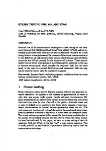
Fig. 1. Utilization sampling for a set of four requests served by a resource.

The next subsections consider three different abstractions for modeling service demand distributions. Section 3.1 and Section 3.2 discuss request-level and session-level characterizations, respectively. Section 3.3 describes how a session group level abstraction can improve characterization. Section 3.4 introduces group service demand models based on phase-type distributions. 3.1

Request Characterization

To begin, consider CPU usage for a single server of a multi-tier architecture ignoring its dependence with other system components. Figure 1 illustrates two possible examples of CPU utilization measurements within a sample period of duration 𝑇1 − 𝑇0 . In both examples, four requests of the same type are served within the time period at instants 𝑎, 𝑏, 𝑐, and 𝑑. The grey boxes illustrate the demands caused by each request and ther busy time within the sample period. Busy time divided by the duration of the sample period is defined as utilization. Consider the general case of 𝑅 request types, it is routine to estimate the mean service demand 𝐸[𝐷𝑟𝑒𝑞,𝑟 ] of type-𝑟 requests using the count of the num(𝑗) ber of type-𝑟 requests served in the 𝑗th sample period, 𝑛𝑟 , and the sampled utilization 𝑈 (𝑗) in that period. Assume that all sample periods have identical length 𝑇1 − 𝑇0 , then utilization and number of completed requests are related in the sample period by the utilization law [3] ( ) 𝑅 (𝑗) ∑ 𝑛𝑟 (𝑗) 𝐸[𝑈 ] = 𝐸[𝐷𝑟𝑒𝑞,𝑟 ] , (1) 𝑇1 − 𝑇0 𝑟=1 where 𝐸[𝑈 (𝑗) ] is computed over all available samples 𝑗 = 1, . . . , 𝐽 and 𝐸[𝐷𝑟𝑒𝑞,𝑟 ] are to be estimated. Estimates for 𝐸[𝐷𝑟𝑒𝑞,𝑟 ] can be readily obtained from (1) using multivariate linear regression [3]. Figure 1 also illustrates the fundamental difficulty of estimating the request service demand distribution from utilization measurements. The two diagrams show different busy times imposed by the requests. Although the distribution of the service demands in the two cases shows different variabilities, the total utilization 𝑈 (𝑗) of the CPU in Figure 1(a) and 1(b) is identical. That is, the

sampling of the utilization values results in information loss with respect to the distribution of the request service times, since it is not possible to discriminate the variability of the two distributions by only looking at the total utilization 𝑈 (𝑗) in the sample period. Unfortunately, 𝑈 (𝑗) is the only information returned by standard CPU monitoring tools, therefore making it difficult to characterize the service demand distribution of requests. This poses a challenge to modeling burstiness and injecting it in a controlled manner into synthetic workloads. Consider the following scheme for estimating the service demand variance that generalizes (1). We observe that 𝑈 (𝑗) (𝑇1 − 𝑇0 ) is the total busy time of the CPU during the 𝑗th sample period and therefore is a summation of the service demands of the requests completed in that interval4 . Assuming request service demands are independent of each other, it follows from the expression for the variance of the sum of independent random variables that 𝑉 𝑎𝑟[𝑈 (𝑗) (𝑇1 − 𝑇0 )] =

𝑅 ∑

𝑛(𝑗) 𝑟 𝑉 𝑎𝑟[𝐷𝑟𝑒𝑞,𝑟 ],

(2)

𝑟=1

However, CPU monitors do not provide direct estimates of the left-hand side variance of (2) thus complicating the estimation of the 𝑉 𝑎𝑟[𝐷𝑟𝑒𝑞,𝑟 ] values. The variance of total busy times can be calculated by measuring the busy times at 𝐽 different samples. However, this approach requires that the numbers of requests belonging to each of the 𝑅 request types be the same for the 𝐽 different (𝑗) (𝑗 ′ ) samples (i.e., 𝑛𝑟 = 𝑛𝑟 for all samples 𝑗 and 𝑗 ′ ). Since enforcing this is unrealistic in practice, the expression given in (2) must be approximated by replacing (𝑗) (𝑗) 𝑛𝑟 with 𝐸[𝑛𝑟 ]. However, this returns very inaccurate results unless there is (𝑗) very low variability in the 𝑛𝑟 values. Summarizing, this discussion highlights a fundamental problem of service variance estimation at the request-level. CPU monitors are unable to provide direct estimates of 𝑉 𝑎𝑟[𝑈 (𝑗) (𝑇1 − 𝑇0 )], thus we need to compute this variance from different sample intervals and this cannot be done accurately by (2). 3.2

Session Characterization

In what follows, we show that changing the level of abstraction in the analysis can significantly help in addressing the limitations of the variance estimation at the request level. Suppose we have 𝑆 session types, the previous observations generalize directly to the estimation of the service demand 𝐷𝑠𝑒𝑠𝑠,𝑠 of a session of type 𝑠 instead of a single request. A generalization of the above analysis (𝑗) (𝑗) leads to formulas almost identical to (1)-(2), but where 𝑛𝑟 is replaced by 𝑛𝑠 which is the number of sessions of type 𝑠 completed in the 𝑗th sample period. While 𝐸[𝐷𝑠𝑒𝑠𝑠,𝑠 ] can be estimated reliably, identical difficulties of the request 4

Henceforth, we ignore the contribution to the busy period of requests that start in a sample period 𝑗 and conclude execution in a different sample period 𝑗 ′ > 𝑗. In fact, it is always possible to consider a sampling granularity sufficiently large to make these effects negligible with respect to the total busy time in the sample period 𝑗.

consumption analysis apply to the estimation of 𝑉 𝑎𝑟[𝐷𝑠𝑒𝑠𝑠,𝑠 ] for sessions. To the best of our knowledge, the estimation problem of higher-order characteristics of the resource consumption has been never addressed in the literature. In the next subsection, we propose the first available general purpose approximation based on a concept of demand characterization for session groups. 3.3

Session Group Characterization Approach

To overcome the difficulties of variance estimation described above, we propose to evaluate the service demand distribution of a group of sessions, instead of each individual session type or request type. These groups can be either suites of pre-existing micro-benchmarks that are already implemented for the multitier system (e.g., the TPC-W workload mixes) or user-defined collections of sessions which perform semantically-homogeneous business operations (e.g., sales sessions, financial and business operations sessions). We assume in the rest of the paper that all groups are already defined by the user according to his knowledge of the multi-tier application characteristics or based on an pre-existing test suite. The fundamental idea behind the group characterization approach is to assume that the variability of resource consumption within a group is mostly due to the heterogeneity of the sessions the group is made of, rather than due to the individual demand variability of each of them. Suppose that a characterization of the mean session service demand 𝐸[𝐷𝑠𝑒𝑠𝑠,𝑠 ] has been obtained, as discussed in the previous subsection, for each type of session 𝑠. Let 𝐷𝑔𝑟𝑝,𝑔 be the service demand of a random session drawn from the group 𝑔. Then ∑ the mean service demand of a random session in the group 𝑔 is 𝐸[𝐷𝑔𝑟𝑝,𝑔 ] = 𝑠∈𝑔 𝜋𝑠,𝑔 𝐸[𝐷𝑠𝑒𝑠𝑠,𝑠 ], where 𝜋𝑠,𝑔 is the probability of drawing a session of type 𝑠 from group 𝑔. Given the assumption of ignoring the complete distribution of the session service demand, we approximate higher-order moments of 𝐷𝑔𝑟𝑝,𝑔 with those of a Markov process jumping randomly between values in the set 𝐸[𝐷𝑠𝑒𝑠𝑠,1 ], . . . , 𝐸[𝐷𝑠𝑒𝑠𝑠,𝑆 ]. That is, we completely characterization session service demands by their means. The properties of this special class of Markov processes are overviewed in Appendix B of [4] and provide the following estimator for the variance of 𝐷𝑔𝑟𝑝,𝑔 : 𝑉 𝑎𝑟[𝐷𝑔𝑟𝑝,𝑔 ] ≈

𝑆 ∑

𝜋𝑠,𝑔 (𝐸[𝐷𝑠𝑒𝑠𝑠,𝑠 ])2 − 𝐸[𝐷𝑔𝑟𝑝,𝑔 ]2 .

(3)

𝑠=1

The last formula translates the concept that a random sampling from a group 𝑔 imposes a service demand variability that is mostly dominated by the variance in the mean request consumption of the different sessions in the group, rather than by each session type variance. Based on 𝐸[𝐷𝑔𝑟𝑝,𝑔 ] and 𝑉 𝑎𝑟[𝐷𝑔𝑟𝑝,𝑔 ] one can immediately fit, according to the procedure discussed in the next subsection, a service demand model that describes the resource consumption the group 𝑔. The above approximation (3) generalizes immediately to higher-order moments 𝑘 according to the relation ∑𝑆 𝑘 𝑘 𝐸[𝐷𝑔𝑟𝑝,𝑔 ] = 𝑠=1 𝜋𝑠,𝑔 (𝐸[𝐷𝑠𝑒𝑠𝑠,𝑠 ]) which provides additional information to fit group service demand models. Finally, this same technique can be applied to different performance attributes at different servers in the multi-tier architecture.

3.4

Group Service Demand Model

Starting from the 𝐸[𝐷𝑔𝑟𝑝,𝑔 ] and 𝑉 𝑎𝑟[𝐷𝑔𝑟𝑝,𝑔 ] values obtained in the previous subsection, we specify group service demand models using phase-type distributions [10], which are a special family of continuous-time Markov chains such that the execution of a job is modeled as a passage through a number of stages with exponentially-distributed service times. Henceforth, we represent phasetype distributions using the (D0 , D1 ) matrix notation [10]. The transitions in D1 are conventionally associated with the completion of service for the job currently in service, while all the remaining transitions describe the accumulation of busy time and are placed in D0 . As an example of the (D0 , D1 ) notation, a twostage Erlang distribution is obtained by summing the samples of two exponential distributions with same mean, which can be expressed as [ ] [ ] −𝜆 𝜆 0 0 D0 = , D1 = (4) 0 −𝜆 𝜆 0 where D0 describes that a job starting in state 1 (first row) first accumulates exponentially-distributed service time with rate 𝜆 as specified by the element (−D0 )1,1 , then it jumps with probability −(D0 )1,2 /(D0 )1,1 = 1 to state 2 where it receives a new exponential service with rate (−D0 )2,2 = 𝜆. Finally, (D1 )2,1 implies that after receiving the second exponential service the job is completed and the following job starts service again from state 1. Details regarding the general fitting of phase-type distributions to match 𝐸[𝐷𝑔𝑟𝑝,𝑔 ] and 𝑉 𝑎𝑟[𝐷𝑔𝑟𝑝,𝑔 ] are given in [4]. By applying the fitting techniques proposed in the appendix to all 𝐸[𝐷𝑔𝑟𝑝,𝑔 ] and 𝑉 𝑎𝑟[𝐷𝑔𝑟𝑝,𝑔 ] pairs generated in the session group characterization we obtain a set of (D0 , D1 ) matrices, henceforth 𝑖,𝑔 denoted by D𝑖,𝑔 = (D𝑖,𝑔 0 , D1 ), that describe the service demand distribution of sessions in group 𝑔 for each performance attribute 𝑖.

4

Benchmark Generation Methodology

This section presents the methodology for automatic generation of bursty benchmarks proposed in this paper. Throughout the following sections, we denote by 𝐵 the benchmark produced as an output by our methodology. As described in Section 2, our approach exploits the SWAT workload generator [12]. SWAT can be easily adapted to compute a group mix vector 𝜸 = (𝛾1 , . . . , 𝛾𝐺 ) defined over the space of the 𝐺 session groups that matches a desired request mix 𝝆 and other properties such as a desired session length distribution. For the purpose of this paper, we assume that 𝜸 has already been computed using SWAT. Therefore, we focus in this section on how to define workload generation mechanisms that insert tunable burstiness in the session service demands. Specifically, we control the sequence in which sessions selected from the 𝐺 session groups are submitted through a session submission policy P. The policy P is specified as a discretetime Markov chain responsible for selecting the session type for the next session to be submitted in a benchmark 𝐵. Controlling the sequence through P allows us to inject a user-specified level of burstiness in 𝐵 while fixing 𝜸.

8

14 simulated session duration

simulated session duration

7 6 5 4 3 2 1 0

0

50 100 150 200 250 300 350 400 450 500 session number

(a) Bursty policy

12 10 8 6 4 2 0

0

50 100 150 200 250 300 350 400 450 500 session number

(b) Traditional policy

Fig. 2. Generation of burstiness using the session submission policy P. Engineered definition of the state transition probabilities in the Markov chain P enables burstiness properties in the session demand.

4.1

Session Submission Policy

The session submission policy P determines the sequence of sessions submitted to the system, both in terms of their type and relative ordering. The policy works as follows. P is a discrete-time Markov chain ⎡ ⎤ 𝑝1,1 𝑝1,2 . . . 𝑝1,𝐺 ⎢ 𝑝2,1 𝑝2,2 . . . 𝑝2,𝐺 ⎥ ⎢ ⎥ P=⎢ . .. . . . ⎥ ⎣ .. . .. ⎦ . 𝑝𝐺,1 𝑝𝐺,2 . . . 𝑝𝐺,𝐺

such that after generating a session from group 𝑔 there is probability 𝑝𝑔,𝑔′ that the following one will be sampled from group 𝑔 ′ . The challenge is how to define these probabilities to match the desired group mix vector 𝜸 and burstiness levels. It is simple to show using standard results for discrete-time Markov chains [3], that if the policy satisfies 𝜸 = 𝜸P, (5) then P generates exactly the desired session group mix 𝜸. Our observation is that (5) leaves considerable flexibility in the definition of P, which we can use to controlled generate burstiness in the demands. An illustrative example of this concept is proposed below.

Burstiness Generation Example. We have considered two policies P𝑡𝑟𝑎𝑑 for a traditional workload generation model and P𝑏𝑢𝑟𝑠𝑡 for a bursty benchmark. These are defined upon 𝐺 = 2 session groups and both satisfy the same requirement 𝜸 = (0.5, 0.5) such that 50% of the sessions are drawn from group 1 and 50% from group 2. Consider the following definition for the two policies: [ ] [ ] 0.50 0.50 0.99 0.01 P𝑡𝑟𝑎𝑑 = , P𝑏𝑢𝑟𝑠𝑡 = 0.50 0.50 0.01 0.99 which both satisfy (5) and differ for the fact that in P𝑏𝑢𝑟𝑠𝑡 there is large 0.99 probability of consecutively sampling sessions from the same group 𝑔. This is

a critical difference because the high probability of sampling sessions from the same state in P𝑏𝑢𝑟𝑠𝑡 implies formation of bursts, as shown by the simulation in Figure 2(a) that are absent in the traditional workload generation model results shown in Figure 2(b). Therefore, by carefully selecting the transition probability in the submission policies we can create radically different behaviors in terms of burstiness. In the next subsection, we explain how the policy P creates service demand burstiness on a per-resource level. 4.2

Composition Step and Benchmark Burstiness Model

This subsection describes the composition step of the proposed methodology. We define Markovian arrival processes (MAPs) [10] to predict the service demand burstiness created at the different system tiers by a benchmark 𝐵 that submits sessions as per a policy P. These models are useful for assessing if P is a good candidate for generating the requested level of burstiness in the system. We remark that MAPs are similar to phase-type distributions, share the same notation, but they are more general as they can also model burstiness; we point to [10] for technical details. Given a policy P and the group demand characterization obtained in Section 3, a burstiness model for a benchmark 𝐵 for performance attribute 𝑖 (e.g., front server CPU, DB CPU, ...) is D𝑖 = 𝑓 𝑖 (D𝑖,𝑔 , P) where the function 𝑓 𝑖 (D𝑖,𝑔 , P) specifies how the burstiness model D𝑖 is constructed from the input parameters. In our methodology, 𝑓 𝑖 (D𝑖,𝑔 , P) is defined as ⎤ ⎤ ⎡ ⎡ 𝑖,1 𝑝1,1 D𝑖,1 𝑝1,2 D𝑖,1 . . . 𝑝1,𝐺 D𝑖,1 D0 0 . . . 0 1 1 1 ⎥ ⎥ ⎢ ⎢ ⎢ 𝑝2,1 D𝑖,2 𝑝2,2 D𝑖,2 . . . 𝑝2,𝐺 D𝑖,2 ⎢ 0 D𝑖,2 1 1 1 ⎥ 0 ... 0 ⎥ ⎥ ⎥ ⎢ ⎢ 𝑖 𝑖 D0 = ⎢ . ⎥ . (6) .. .. .. .. . . .. ⎥ , D1 = ⎢ .. ⎥ ⎥ ⎢ ⎢ .. . . . . . . . ⎦ ⎦ ⎣ ⎣ 0

0 . . . D𝑖,𝐺 0

𝑝𝐺,1 D𝑖,𝐺 𝑝𝐺,2 D𝑖,𝐺 . . . 𝑝𝐺,𝐺 D𝑖,𝐺 1 1 1

The D𝑖0 matrix specifies that the service demands of a session generated by a group 𝑔 follow its service demand distribution model D𝑖,𝑔 ; the D𝑖1 matrix describes the modulation due to the session submission policy P. The fundamental result achieved by the composition step described above is that the benchmark burstiness model D𝑖 defined for a performance attribute 𝑖 lets us evaluate by closed-form analytical expressions the burstiness in the service demands for performance attribute 𝑖 due to the benchmark 𝐵. Under positive autocorrelations, burstiness levels for a performance attribute can be evaluated and specified by the index of dispersion [10] ∑∞ 𝐼 = 𝐶𝑉 2 (1 + 2 𝑘=1 𝜌(𝑘)), where 𝐶𝑉 is the coefficient of variation of the service demands, 𝜌(𝑘) is the lag-𝑘 autocorrelation coefficient of the service demands, see [10, 15] for further

information. The autocorrelation function 𝜌(𝑘) is often used as a more accurate burstiness descriptor than the index of dispersion 𝐼, therefore we consider both in the rest of the paper. For the model (D𝑖0 , D𝑖1 ), the service demand of performance attribute 𝑖 has moments 𝐸[𝐷𝑖𝑘 ] = 𝑘!𝝅𝑒 (−D𝑖0 )−𝑘 e,

(7)

where 𝐸[𝐷𝑖𝑘 ] is 𝑘th moment of the service demand of the benchmark 𝐵 on performance attribute 𝑖, and 𝝅 𝑒 = 𝝅 𝑒 (−D𝑖0 )−1 D𝑖1 describes the equilibrium state of the MAP. The index of dispersion of performance attribute 𝑖 which quantifies its burstiness levels is given by ( ) 𝝅𝑒 𝑖 𝑖 𝑖 𝑖 𝐼(𝑖) = 1 + 2 𝐸[𝐷𝑖 ] − D (D + D1 + e𝝅𝑒 )D1 e . (8) 𝐸[𝐷𝑖 ] 1 0 Equation (8) shows the full potential of our model-based methodology: starting from the characterization of the session groups and of the submission policy, we are able to evaluate the burstiness of the service demands for all performance attributes of all servers before running the benchmark. This fundamental result is exploited below to search for a submission policy P that introduces the desired burstiness in the system. 4.3

Searching for a Submission Policy to Match Burstiness

Finally, we use a nonlinear optimization program to search for policy P that provides the desired levels of burstiness in the service demands. Our approach is to evaluate iteratively the burstiness generated by several policies P and choose the one that is closest to the target burstiness specified by the user. Additionally, the optimization is constrained on the benchmark 𝐵 generating the predefined session group mix 𝜸. Due to limited space, we exemplify the generation of burstiness for a performance attribute 𝑖 to match a given index of dispersion value 𝐼𝑡𝑎𝑟𝑔𝑒𝑡 (𝑖). This is achieved by the following nonlinear optimization program min 𝑧 = ∣𝐼(𝑖) − 𝐼𝑡𝑎𝑟𝑔𝑒𝑡 (𝑖)∣ 𝑠.𝑡. P

(D𝑖0 , D𝑖1 ) = 𝑓 𝑖 (D𝑖,𝑗 , P); ( ) −1 𝐼(𝑖) = 1 + 2 𝐸[𝐷𝑖 ] − 𝐸[𝐷𝑖 ] 𝝅 𝑒 D𝑖1 (D𝑖0 + D𝑖1 + e𝝅 𝑒 )D𝑖1 e ; 𝐸[𝐷𝑖 ] = 𝝅 𝑒 (−D𝑖0 )−1 e;

𝝅 𝑒 (−D𝑖0 )−1 D𝑖1 ;

(9) (10) (11) (12)

𝝅𝑒 = Pe = e;

(13) (14)

P ≥ 0;

(15)

𝜸P = 𝜸;

(16)

where e is a column vector of size 𝐺 composed of all ones. The search is on the entries of the policy P which minimize the difference between the target index

of dispersion and the one estimated for the service demands of performance attribute 𝑖 based on the 𝑓 𝑖 (D𝑖,𝑗 , P) mapping. The constraints are of three types: (11)-(13) are the formulas for computing the index of dispersion 𝐼 applied to the burstiness model (D𝑖0 , D𝑖1 ); (14)-(15) impose that P is a stochastic matrix; finally, (16) imposes the session group mix 𝜸. The nonlinear program (9)-(16) returns a session submission policy P that achieves the stated goal of this paper of creating a benchmark 𝐵 with the desired burstiness 𝐼𝑡𝑎𝑟𝑔𝑒𝑡 in a performance attribute 𝑖. Theoretically, there are no limits to the maximum achievable index of dispersion in a server, yet very large values create long-range dependence that requires very long executions of the benchmark in order to realize the desired level of burstiness [7]. Although the optimization program is nonlinear, we have found it in practice easy to solve. In the experiments reported in Section 5, we always obtained good solutions in less than one minute. If one is interested in generating controlled burstiness in several performance attributes simultaneously, it is possible either to consider multiple objective functions, one for each performance attribute of interest, or to inject burstiness into the aggregate service demand of the sessions, i.e., the round-trip time of a session when executed in isolation on the system. For instance, for a system with a front server and a database server, the aggregate service demand is 𝐴 = 𝐷𝑓 𝑟𝑜𝑛𝑡 + 𝐷𝑑𝑏 , where 𝐷𝑓 𝑟𝑜𝑛𝑡 and 𝐷𝑑𝑏 are service demands at the two servers. We illustrate the effectiveness of this approach in the first case study proposed in the next section.

4.4

Generating Dynamic Bottleneck Switches

Finally, we discuss the relation between generation of burstiness and dynamic bottleneck switches. As observed in [15], significant performance degradation due to burstiness is observed mainly if there are dynamic bottleneck switches between the resources that create adverse queueing conditions. For instance, in the TPC-W benchmark it is observed that the Best Seller transaction places a very high demand at the database server CPU while in execution. Due to burstiness, several Best Seller transactions may be scheduled for execution consecutively, this results in the front server CPU and the database server CPU cyclically alternating the role of bottleneck in the system. From the above discussion, it follows naturally that the basic requirement for the benchmark 𝐵 to create dynamic bottleneck switches between 𝑀 performance attributes is that there exist for each attribute 𝑚 = 1, . . . , 𝑀 at least a group 𝑔 that places an average service demand 𝐸[𝐷𝑔𝑟𝑝,𝑔 ] on 𝑚 that is bigger than the average demand placed on any other performance attribute in the system. This implies that when the policy P starts to draw consecutively from the group 𝑔 as in the example of Section 4.1, then resource 𝑚 would become the system bottleneck until P chooses another group to sample from. Our technique exploits the service demand models to construct benchmarks that will cause a bottleneck switch. One such benchmark is discussed in detail in Section 5.

5

Validation Experiments

To show that our benchmark generation approach is effective in creating controlled burstiness, we present a case study that considers a particular combination of the browsing, ordering, and shopping mix benchmarks of TPC-W. The resulting benchmark 𝐵 is run on a real testbed; we consider CPU usage at the different computing nodes as performance attributes. The testbed consists of a front server node, a database node, and a client node connected by a nonblocking Ethernet switch that provides a dedicated 1 Gbps connectivity between any two machines in the setup. The front server and database nodes are used to execute the TPC-W bookstore application implemented at Rice University [1]. The client node is dedicated for running the httperf Web request generator. This was configured to emulate multiple concurrent sessions in our experiments. The httperf generator has features such as non-blocking socket calls that allow it to stress servers and sustain overloads without the need for multiple client nodes. All nodes in the setup contain an Intel 2.66 GHZ Core 2 CPU and 2 GB of RAM. The Windows perfmon utility is used to gather CPU, disk, memory, and network usage at the server nodes; httperf provides detailed logs of end user response times. In all our experiments we noticed very little disk, paging, and network activity. Throughout the experiments, we have used pre-existing test suites created to follow the shopping, browsing, and ordering mixes specified by TPC-W. The matrix P that results from the benchmark generation step is used to construct a trace of 10,000 sessions with desired mix and burstiness and that combines the three test suites. Finally, httperf is used to submit the session trace to the system. Due to limited space, we report below only two case studies, but we remark that we have considered several other experiments resulting in qualitatively similar results to those reported below. 5.1

Validation of Service Demand and Burstiness Models

We first consider a benchmark 𝐵 defined only by a mix of sessions of shopping (𝑠ℎ𝑝) and ordering (𝑜𝑟𝑑) type. The mix is balanced with group request mix 𝛾𝑠ℎ𝑝 = 𝛾𝑜𝑟𝑑 = 0.50, and we assume the session submission policy P is assigned such that shopping (resp. ordering) sessions have a probability 𝑝𝑠ℎ𝑝,𝑠ℎ𝑝 = 0.995 (resp. 𝑝𝑜𝑟𝑑,𝑜𝑟𝑑 = 0.995) that the next session generated after them will be again of shopping (resp. ordering) type, i.e., [ ] 0.995 0.005 P= 0.005 0.995 The aim of this case study is to validate the prediction accuracy of the models proposed in Sections 3 and 4. Since it is hard to obtain direct measurement of the service demands, we focus on prediction of utilization and aggregate service demand measurements for the sessions executed in isolation on the system. For the group service demand model definition, we have run in isolation the shopping and ordering benchmarks and estimated the mean session demands

front server shopping mean CV measured 0.290 0.575 phase-type 0.290 0.575 ordering mean CV measured 0.131 0.805 phase-type 0.131 0.805

demand skew 2.671 1.665 skew 1.797 1.328

DB server demand mean CV skew 0.097 7.590 4.509 0.097 7.591 3.161 mean CV skew 0.623 1.761 2.530 0.623 1.340 2.002

Table 1. Group service demand models for CPU. Means are expressed in seconds.

1

0.6

autocorrelation coefficient

cdf P[ round trip ≤ t]

0.7 0.6 0.5 0.4 0.3 0.2

0.4 0.3 0.2 0.1 0 −0.1

1

2

3 t

(a) CDF Aggregate mand (sec)

4

−0.3

model trace sample path

0.5 0.4 0.3 0.2 0.1 0 −0.1 −0.2

−0.2

0.1 0

model trace sample path

0.5

0.8

autocorrelation coefficient

trace model

0.9

0

10

20

30

40

50 lag

60

70

80

90 100

0

10

20

30

40

50 lag

60

70

80

90 100

De- (b) Front Server Utilization (c) DB Server Utilization

Fig. 3. Experimental results for the mix of shopping and ordering sessions.

for each of the session types used in the these mixes. Table 1 presents results. The table shows the estimated moments for the different CPU service demands and the respective moments of the phase-type distributions we have fitted; the number of states we have used in the phase-type models is always less than 7. The results indicate that the phase-type distributions match very well mean and CV of the measured group service demands, while they slightly underestimate the value of the skewness probably due to the difficulty in modeling in a Markovian setting the nearly-deterministic demand of individual session types. Using the phase-type distributions D𝑖,𝑔 and the policy P, we have then defined the MAPs that describe the CPU service demands at the front server D𝑓 𝑠 and at the database server D𝑑𝑏 . We have also defined a MAP to describe the aggregate service demand of the sessions generated by 𝐵: assuming that each session visits the front server and database server once before completing execution, the MAP that captures the aggregate service demands has (D0 , D1 ) representation, denoted by (A0 , A1 ), which is a simple combination of D𝑓 𝑠,𝑠ℎ𝑝 , D𝑑𝑏,𝑠ℎ𝑝 , D𝑓 𝑠,𝑜𝑟𝑑 , D𝑑𝑏,𝑜𝑟𝑑 weighted by the probabilities 𝑝𝑜𝑟𝑑,𝑜𝑟𝑑 and 𝑝𝑠ℎ𝑝,𝑠ℎ𝑝 similarly to (6). Figure 3(a) compares the cumulative distribution function (CDF) for the aggregate service demand of the benchmark 𝐵 sessions with the ones predicted by the (A0 , A1 ) model. The distribution of the MAP matches the empirical distribution of the aggregate service demand very well, thus suggesting the effectiveness of our demand models in capturing the distribution of the service demands. Using (A0 , A1 ), we have also compared the burstiness of the aggregate service demands predicted by the model with the one measured on the real system using the autocorrelation function as a descriptor of burstiness [17]. The

result (not shown graphically due to limited space) indicates good prediction accuracy, with the aggregate service demand autocorrelation coefficients quickly decaying to zero for both the model and the measurements, and with the lag-1 coefficient being 𝜌(1) = 0.028 for the measured aggregate service demands and 𝜌(1) = 0.039 for the (A0 , A1 ) model. The results of the aggregate service demand analysis suggest that the models developed in Sections 3 and 4 capture service demands very well, otherwise it would be hard to predict accurately aggregate service demands distribution and burstiness for sessions of the benchmark 𝐵. To further validate accuracy, we have also performed a trace-driven analysis of the system to compare the properties of the measured utilizations with those predicted by the MAP models. Figure 3(b)-(c) show the autocorrelation function of the measured and modeled CPU utilizations for the front server and database server, respectively. The autocorrelations of the model are estimated by averaging the autocorrelations over 100 random experiments; conversely, the sample path curve shows a representative example of autocorrelation estimate for one of these random experiments. The results are qualitatively similar for both servers suggesting that the session generation policy impacts equally on the two tiers. For low lags, model and sample path autocorrelations are in very good agreement with the TPC-W trace. Low lags are the most significant for burstiness, as they measure the similarities of consecutive sessions that pack into bursts, while high lags are mostly related to the length of these bursts. The autocorrelation coefficient values for lags greater than 10 seem instead to suffer significant noise due to limited size of the measurement due to the utilization sampling; the presence of noise is proved by the difference between the sample path curve and the model results averaged over 100 experiments. Yet, the good agreement of the sample path with the trace proves that sample paths of the MAP model are representative of system behavior observed in real experiments. Summarizing, the experiments in this section suggest that the proposed phase-type and MAP models can summarize and predict effectively the properties of the demands in both the pre-existing benchmark suites and in the composed benchmark 𝐵. The next case study focuses instead on the quality and practical impact of the burstiness generation methodology. 5.2

Generation of Burstiness and its Impact

We consider a mix of ordering, browsing and shopping sessions, but we now focus on generating benchmarks to evaluate the performance of the TPC-W system under burstiness conditions. The results presented in this section prove that this can be done successfully with the proposed methodology and prove the existence of scalability problems for systems that are not revealed by executions of traditional benchmarks without burstiness. Solving the nonlinear optimization program defined in Section 4.3 with the fmincon function of MATLAB 7.6.0, we have created two session submission policies P𝑛𝑜𝑛−𝑏𝑢𝑟𝑠𝑡 and Pℎ𝑖𝑔ℎ−𝑏𝑢𝑟𝑠𝑡 that both combine browsing (𝑏𝑟𝑜), shopping (𝑠ℎ𝑝) and ordering (𝑜𝑟𝑑) sessions with group mix 𝛾𝑏𝑟𝑜 = 0.014 and 𝛾𝑠ℎ𝑝 =

0.9

0.9

0.8

0.8

0.7

0.7

0.6 0.5 0.4

front db

0.5 0.4 0.2

front db

0.1 0 0

50

0.1 0 100 150 utilization sample

200

250

20 50

100 150 200 sample interval number high burstiness (I=50)

250

300

50

100 150 200 sample interval number

250

300

60

0.3

0.2

40

0 0

0.6

throughput

0.3

60 throughput

1

utilization

utilization

no burstiness (I=0) 1

0

50

100 150 200 utilization sample

250

300

(a) 𝐼 = 1.14, No Burstiness (b) 𝐼 = 50, High Burstiness

40 20 0 0

(c) Throughput

250

bro shp ord total

200

number of requests in the system

number of requests in the system

Fig. 4. CPU utilization and session throughput for the bursty and the nonbursty benchmarks.

150 100 50 0

0

50

100 150 200 sample period of arrival

250

(a) No Burstiness

300

250

bro shp ord total

200 150 100 50 0

0

50

100 150 200 sample period of arrival

250

300

(b) High Burstiness

Fig. 5. Time series showing the number of requests that are concurrently served by the multi-tier application during each experiment. Measurements are taken at the instant of arrival of a new request.

𝛾𝑜𝑟𝑑 = 0.493. The group mix is essentially the same as in Section 5.1, but there is in our workload also a component of about 100 − 200 browsing sessions which shows that our methodology can apply also to combination of more than two test suites. Only a limited fraction of browsing sessions is used to avoid having a bottleneck switch due to this test suite and not to the policy 𝑃 that we want to validate. In fact, the browsing mix is known to impose fluctuations between front server and database server CPU utilizations [15]. The two policies differ only with respect to the index of dispersion values in the aggregate demand. The non-bursty benchmark defined by P𝑛𝑜𝑛−𝑏𝑢𝑟𝑠𝑡 has index of dispersion in the aggregate demand 𝐼 = 1.14, which is a case corresponding to the removal of burstiness by imposing a zero value for all the autocorrelation coefficients5 . This also results in negligible burstiness in the service demands at the server CPUs: the expected index of dispersions at the front server CPUs and at the database server CPUs are 𝐼𝑓 𝑠 = 0.82 and 𝐼𝑑𝑏 = 2.11, respectively. The scale of the index of dispersion is comparable to the scale of the squared coefficient of variation 𝐶𝑉 2 , thus 𝐼 < 1 indicates low or no burstiness, whereas 𝐼 of the order of tens or more generally stands for high burstiness. The high-burstiness benchmark defined by Pℎ𝑖𝑔ℎ−𝑏𝑢𝑟𝑠𝑡 has index of dispersion 𝐼 = 50 in the aggregate demand, which 5

2 In fact, in this workload 𝐶𝑉∑ = 1.14, thus 𝐼 = 𝐶𝑉 2 implies from the definition of the index of dispersion that ∞ 𝑘=1 𝜌(𝑘) = 0.

bro shp ord

bro shp ord

1E5 mean response time [ms]

mean response time [ms]

1E5

1E4

1E3

1E4

1E3

1E2 1E2

0

50

100 150 200 sample period of arrival

250

300

0

50

1

3000

1e−1

2500

1e−2 1e−3 no burstiness burstiness, I=50

1e−4

250

300

(b) High Burstiness

number of DB locks

CCDF: 1−F(t)

(a) No Burstiness

100 150 200 sample period of arrival

1e−5

no burstiness burstiness I=50

2000 1500 1000 500

0

1e1

1e2 1e3 1e4 t − request response times

1e5

(c) CCDF Response Times

0

0

50

100 150 200 sample interval number

250

300

(d) Locks

Fig. 6. Performance effects of the dynamic bottleneck switch.

creates large burstiness both in the aggregate and per-server service demands. The expected index of dispersion for the front server CPUs is 𝐼𝑓 𝑠 = 597.34 and for the database CPUs is 𝐼𝑑𝑏 = 2242.9. Figure 4 compares the performance impact of the two benchmarks on the TPC-W system for an experiment with Poisson session arrivals and multiple concurrent sessions in execution. Even though both benchmarks have the same session type mix, session inter-arrival time distribution, and almost identical server CPU utilizations, the bursty benchmark stresses the system differently than the non-bursty benchmark. From Figures 4(a)-(b), the front and database server CPU utilizations display a more random pattern for the bursty benchmark. As expected, Figures 5(a)-(b) show that these patterns are also reflected immediately in the number of active requests which varies according to the active session group. In all plots, the sampling granularity is of 15 seconds. The bursty workload adversely impacts the responsiveness and throughput of the system. From Figures 4(a)-(b), the maximum utilization of the database server is higher for the bursty workload than the non-bursty workload. From Figure 4(b), it can be observed that the database server is saturated from sample 0 to sample 100 and from sample 200 to sample 300. This behavior is absent in the non-bursty workload. The heightened contention for the database server causes the number of concurrent sessions in the system to rise beyond the limit imposed by the sizes of the front server thread pool and listen queue. As a result, the front server drops several connections leading to a 25% drop in request throughput relative to the non-bursty case. This is evident also in Figure 4(c) which illustrates the

number of successfully completed sessions over time. The figure clearly indicates that for the bursty workload the throughput of successfully completed sessions drops below acceptable levels frequently when the database is saturated, whereas throughput is steady in the non-bursty case. The experiments also reveal that burstiness can cause bottleneck switches that can introduce unpredictable transient behavior into the system. From Figure 4(b), the system bottleneck switches from the database server to the front server near the 100th sample. In contrast, from Figure 4(a), there is no bottleneck switch with the non-bursty workload. The bottleneck switch is caused due to a transition from the database intensive browsing and ordering sessions to the front server intensive shopping sessions in the bursty workload. It can be observed from Figure 5(b) that there is a significant accumulation of shopping sessions in the system exactly at the time of the bottleneck switch, as visible around sample 110 by the number of ordering sessions decreasing while shopping sessions accumulate at a fast rate. This large accumulation of shopping sessions is caused because of these sessions being delayed by the last of the bro wsing and ordering sessions at the database server. As a result of this dynamic, it takes the system around 12 minutes spanning the period from sample 110 to sample 160 to significantly reduce the backlog of shopping sessions. This type of unstable transient behavior was not observed with the non-bursty workload and represents a unique feature of burstiness that cannot be exposed with non-bursty submission policies or by running the two benchmarks in isolation. Specifically, such techniques would result in no backlog for the shopping sessions and therefore would never exhibit the properties highlighted in Figure 5(b). Furthermore, the accumulation of the backlog due to bottleneck switch dominates the response time results presented in Figure 6. Figure 6(a)-(b) show the mean response times of requests over time. Specifically, Figure 6(b) shows many important points for our analysis. First, ordering and browsing sessions have considerably larger response times when executed on the system from sample 0 to sample 110 and from sample 210 to 300 than in the corresponding periods of the non-bursty benchmark in Figure 6(a). This suggests that burstiness is more critical for the response times of browsing and ordering sessions which are both database intensive and hence place a strongest congestion level if they are executed in the system without shopping sessions interleaved between them that can alleviate the bottleneck by shifting more load on the front server. The second fundamental observation is that, from sample 110 to 130, the first shopping sessions entering into the system receive dramatically large response times due to the bottleneck switch phenomena. Progressively, as the backlog is flushed response times display a reducing trend. From sample 160 the response times of shopping sessions is lower than in the no-burstiness case, suggesting that the front server can cope well with this level of parallelism for shopping sessions. Finally, it is important to observe that the introduction of burstiness has eventually resulted into a generalized spread of delays, with the exception of the small range from sample 160 to 200. Figure 6(c) compares request response times under the bursty and non-bursty benchmarks: most of the requests without burstiness are

served in less than 10 seconds, however more than 20% of the requests in the bursty benchmark require at least 100 seconds to be completed, thus making the point that our approach is better suited than other approaches for stress testing. Finally, Figure 6(d) plots for both the bursty and non-bursty benchmark the number of database queries that are waiting to acquire locks for rows in the database. From the figure the bursty workload causes heightened contention for locks after the first bottleneck switch. Recall that the bottleneck switch was caused by the arrival of a burst of shopping sessions. Furthermore, shopping sessions rely on a common set of data. Consequently, the burst of shopping sessions causes increased locking activity in the system while accessing this common data set. In contrast, the non-bursty workload does not contain significant bursts of sessions of similar type and as a result does not expose heightened lock contention and the associated performance implications.

6

Conclusion

We have proposed a model-based methodology for the automatic generation of benchmarks with customizable levels of burstiness in the service demands. Our methodology extends existing approaches for automatic synthesis of benchmarks such as SWAT [12]. Experiments on a real TPC-W testbed have shown that the proposed models are very accurate in predicting the service demands and their burstiness at the different tiers of the architecture. We have shown a case where the ordering and shopping mixes of TPC-W have been combined to inject controlled burstiness in the demands resulting in critical stress conditions for performance that are not shown by non-bursty combinations of the two mixes. We plan to further develop and validate this new approach within a framework that aims to characterize, synthesize, and predict the impact of burstiness on multi-tier systems. We want to further investigate in detail the various kinds of system level degradations that can be caused by burstiness and study how to specify groups given different alternatives. Finally, a point that needs to be investigated in future work is to assess the validity of the proposed techniques in presence of long lived sessions, such as those performing long database queries that may take several minutes to execute and may suffer considerable variability in running times. Under these conditions, it may be needed to define ad-hoc estimators for the demand variance of such transactions. Given such variance estimates, a possible approach to extend our methodology could be to isolate these sessions into separate groups and have a phase-type distribution of their demand, however further work is needed to assess the feasibility of this approach.

Acknowledgments This research was partially funded by the InvestNI/SAP project MORE and by grants from the Natural Sciences and Engineering Research Council of Canada (NSERC). We thank Stephen Dawson for helpful feedback during the preparation of this work.

References 1. C. Amza, A. Ch, A. L. Cox, S. Elnikety, R. Gil, K. Rajamani, E. Cecchet, and J. Marguerite. Specification and implementation of dynamic web site benchmarks. Proc. of WWC workshop, Austin, TX, Nov 2002. 2. P. Barford and M. Crovella. Generating Representative Web Workloads for Network and Server Performance Evaluation. ACM PER, 26(1), 151-160, 1998. 3. G. Bolch, S. Greiner, H. de Meer, K. S. Trivedi. Queueing Networks and Markov Chains. Wiley, 2006. 4. G. Casale, A. Kalbasi, D. Krishnamurthy, and J. Rolia. Automated Stress Testing of Multi-Tier Systems by Dynamic Bottleneck Switch Generation. University of Calgary Technical Report SERG-2009-02, April 2009. http://people.ucalgary.ca/∼ dkrishna/SERG-2009-02.pdf 5. G. Casale, A. Kalbasi, D. Krishnamurthy, and J. Rolia. Automatically Generating Bursty Benchmarks for Multi-Tier Systems. Presented at the 2nd Workshop on Hot Topics in Measurement and Modeling of Computer Systems (HotMetrics), Jun 2009, published online at http://www.sigmetrics.org /conferences/sigmetrics/2009/workshops/papers hotmetrics/session2 1.pdf 6. G. Casale, N. Mi, and E. Smirni. Bound analysis of closed queueing networks with workload burstiness. In Proc. of ACM SIGMETRICS, 13–24, 2008. 7. M. Crovella, L. Lipsky. Long-Lasting Transient Conditions in Simulations with Heavy-Tailed Workloads. Winter Simulation Conference, 1005-1012, 1997. 8. J. J. Dujmovic, Universal benchmark suites, In Proc. of MASCOTS, 197-205, 1999. 9. R. Grace, The benchmark book. Prentice Hall, 1996. 10. A. Heindl. Traffic-Based Decomposition of General Queueing Networks with Correlated Input Processes. Ph.D. Thesis, Shaker Verlag, Aachen, 2001. 11. K. Kant, V. Tewary, and R. Iyer. An Internet Traffic Generator for Server Architecture Evaluation. In Proc. CAECW, Jan 2001. 12. D. Krishnamurthy, J. A. Rolia, and S. Majumdar. A synthetic workload generation technique for stress testing session-based systems. IEEE Trans. Soft. Eng., 32(11):868–882, Nov 2006. 13. U. Krishnaswamy, D. Scherson, A framework for computer performance evaluation using benchmark sets. IEEE Trans. on Computers, 49(12):1325-1338, Dec 2000. 14. W. E. Leland, M. S. Taqqu, W. Willinger, and D. V. Wilson. On the self-similar nature of ethernet traffic. IEEE/ACM Trans. on Networking, 2(1):1–15, 1994. 15. N. Mi, G. Casale, L. Cherkasova, and E. Smirni. Burstiness in multi-tier applications: Symptoms, causes, and new models. In Proc. of Middleware, LNCS 5346, 265–286, 2008. 16. N. Mi, G. Casale, L. Cherkasova, and E. Smirni. Injecting Realistic Burstiness to a Traditional Client-Server Benchmark. In Proc. of ICAC, June 2009, 149–158. 17. N. Mi, Q. Zhang, A. Riska, E. Smirni, and E. Riedel. Performance impacts of autocorrelated flows in multi-tiered systems. Perf. Eval., 64(9-12):1082–1101, 2007. 18. A. Riska and E. Riedel. Long-range dependence at the disk drive level. In Proc. of QEST, 41–50, 2006. 19. J. Rolia, D. Krishnamurthy, A. Kalbasi, and S. Dawson. Resource demand modeling for complex services, (under submission).