Automatic Synthesis of Distributed Transition ... - Semantic Scholar

Automatic Synthesis of Distributed Transition Systems

Von der Fakultät Informatik, Elektrotechnik und Informationstechnik der Universität Stuttgart zur Erlangung der Würde eines Doktors der Naturwissenschaften (Dr. rer. nat.) genehmigte Abhandlung

Vorgelegt von Alin S ¸ tef˘ anescu aus Slatina, Rumänien

Vorsitzender des Prüfungsausschusses: Prof. Dr. Volker Diekert Hauptberichter: Prof. Dr. Javier Esparza Mitberichter: Prof. Dr. Colin Stirling Tag der mündlichen Prüfung:

13.2.2006

Institut für Formale Methoden der Informatik Universität Stuttgart 2006

trib

Automatic Synthesis of

Dis

ed ut

Alin S¸tef˘anescu March 7, 2006

Transition Systems

Abstract This thesis investigates the synthesis problem for two classes of distributed transition systems: synchronous products and asynchronous automata. The underlying structure of these models consist of local automata synchronizing on common actions. The synthesis problem discussed is as follows: Given a global specification as a transition system TS and a distribution pattern ∆, find a distributed transition system over ∆ whose global state space is ‘equivalent’ to TS . As criteria for the correctness of the (distributed) implementation vs. the specification (i.e., their ‘equivalence’) we use: transition system isomorphism, language equivalence, and bisimilarity respectively. In particular, the synthesis of asynchronous automata modulo language equivalence is a notoriously hard problem solved by Zielonka at the end of the 80s. One of the motivations behind our work was to bring this theory closer to practical applications. From the theoretical point of view, we conduct a detailed analysis of the synthesis problem for both models of distributed systems, look at effective algorithmic approaches and draw a map of computational complexity results. E.g., we provide several matching lower and upper complexity bounds for the distributed implementability problem. From the practical perspective, we provide prototype implementations for most of the synthesis algorithms discussed in the thesis. Moreover, we offer assistance when a given specification is not distributable by trying to modify this specification such that distributed synthesis can be applied. By using several heuristics to overcome the classical state space explosion, we are able to automatically generate small distributed algorithms for problems such as mutual exclusion.

Zusammenfassung Diese Dissertation erforscht das Syntheseproblem f¨ ur zwei verschiedene Arten von verteilten Transitionssysteme: synchrone Produkte und asynchrone Automaten. Diese Modelle bestehen aus lokalen Automaten, die sich u ¨ber gemeinsame Aktionen synchronisieren. Das betrachtete Syntheseproblem ist Folgendes: F¨ ur ein gegebenes Transitionssystem TS und eine Verteilungsstruktur ∆ sucht man ein verteiltes Transitionssystem u ¨ber ∆ mit einem globalen Zustandraum “äquivalent” zu TS . Als Kriterien f¨ ur die Korrektheit der ¨ Implementierung bez¨ uglich der Spezifikation (d.h., ihre “Aquivalenz”), verwenden wir Transitionssystem-Isomorphismus, Sprachenäquivalenz bzw. Bisimilarität. Insbesondere ist die Synthese der asynchronen Automaten Modulo-Sprachenäquivalenz ein bekanntes hartes Problem, das von Zielonka Ende der 80iger Jahre gelöst wurde. Einer der Beweggr¨ unde hinter unserer Arbeit war diese Theorie näher an praktische Anwendungen zu holen. Aus theoretische Sicht leiten wir eine ausf¨ uhrliche Analyse des Syntheseproblems f¨ ur beide Modelle der verteilten Systeme, betrachten wirkungsvolle algorithmische Verfahren ¨ und erarbeiten eine Ubersicht der Berechnungskomplexität. So z.B. stellen wir einige untere und obere Komplexitätsgrenzen f¨ ur das verteilte Implementierungsproblem zur Verf¨ ugung. Von einer praktischen Ansicht leifern wir Prototypimplementierungen f¨ ur die meisten Synthesealgorithmen, die in diese Dissertation besprochen werden. Außerdem bieten wir Unterst¨ utzung an, falls eine gegebene Spezifikation nicht verteilbar ist und versuchen, sie zu ändern, so daß verteilte Synthese möglich wird. Indem wir einige Heuristiken verwenden, zum der klassischen Zustandraumsexplosion zu u ¨berwinden, sind wir in der Lage, kleine verteilte Algorithmen f¨ ur Probleme, wie z.B. der gegenseitige Ausschluß (Mutex), automatisch zu erzeugen.

Acknowledgments In the first place I would like to thank to my supervisor Javier Esparza, for all the kindness he has showed, the model he has been, and all the help he has provided to make this work come into being. Then, there is a long list of people I am indebted to regarding this work and my formation. I will mention here only a few of them: Keijo Heljanko, Barbara König, Vitali Kozioura, Ioana and Laurent¸iu Leu¸stean, Rémi Morin, Anca Muscholl, Claus Schröter, Stefan Schwoon, Gheorghe S¸tef˘anescu, Ljiljana and Joseph Spadavecchia, Marin Tolo¸si. Moreover, to all the friends in M¨ unchen, Edinburgh, and Stuttgart I am grateful for the moments we shared. Also, I thank Stefan Leue for the support during the last part of the writing-up process and Colin Stirling for accepting to referee this thesis. I owe a deep debt of gratitude to my family for love, support, and understanding.

Declaration I declare that this thesis was composed by myself, that the work contained herein is my own except where explicitly stated otherwise in the text, and that this work has not been submitted for any other degree or professional qualification except as specified.

(Alin S ¸ tef˘ anescu)

This thesis is dedicated to my daughter Anastasia Because of Anastasia, the thesis may have a couple of sections less. Because of the thesis, Anastasia had her father around less.

This thesis is also dedicated to my wife Cornelia Because of Cornelia, I have now both the thesis and Anastasia.

Contents 1 Introduction 1.1 The Synthesis Problem . . . . . . . . . . . . . . . . . . . . . . . . . . . . . 1.2 A Small Example . . . . . . . . . . . . . . . . . . . . . . . . . . . . . . . . 1.3 The Contribution of this Thesis . . . . . . . . . . . . . . . . . . . . . . . . 2 Preliminaries 2.1 Basic Notions and Notations 2.1.1 Set Theory . . . . . 2.1.2 Algebraic Notions . . 2.1.3 Formal Languages . . 2.1.4 Graph Theory . . . . 2.2 Transition Systems . . . . . Discussion . . . . . . . . . . . . .

. . . . . . .

. . . . . . .

. . . . . . .

. . . . . . .

. . . . . . .

. . . . . . .

. . . . . . .

. . . . . . .

. . . . . . .

. . . . . . .

. . . . . . .

. . . . . . .

. . . . . . .

3 Distributed Transition Systems and the Synthesis 3.1 Trace Theory . . . . . . . . . . . . . . . . . . . . . 3.2 Distributed Transition Systems . . . . . . . . . . . 3.2.1 Distributions . . . . . . . . . . . . . . . . . 3.2.2 Synchronous Products of Transition Systems 3.2.3 Asynchronous Automata . . . . . . . . . . . 3.3 Shapes . . . . . . . . . . . . . . . . . . . . . . . . . 3.3.1 Diamonds et al. . . . . . . . . . . . . . . . . 3.3.2 Synchronous Products of Transition Systems 3.3.3 Asynchronous Automata . . . . . . . . . . . 3.4 Languages . . . . . . . . . . . . . . . . . . . . . . . 3.4.1 Final States . . . . . . . . . . . . . . . . . . 3.4.2 Traces of Diamonds . . . . . . . . . . . . . . 3.4.3 Synchronous Products of Transition Systems 3.4.4 Asynchronous Automata . . . . . . . . . . . 3.4.5 Comparative Expressiveness . . . . . . . . . 3.5 The Synthesis Problem . . . . . . . . . . . . . . . . Discussion . . . . . . . . . . . . . . . . . . . . . . . . . . i

. . . . . . .

. . . . . . .

. . . . . . .

. . . . . . .

. . . . . . .

. . . . . . .

Problem . . . . . . . . . . . . . . . . . . . . . . . . . . . . . . . . . . . . . . . . . . . . . . . . . . . . . . . . . . . . . . . . . . . . . . . . . . . . . . . . . . . . . . . . . . . . . . . . . . . . . .

. . . . . . .

. . . . . . . . . . . . . . . . .

. . . . . . .

. . . . . . . . . . . . . . . . .

. . . . . . .

. . . . . . . . . . . . . . . . .

. . . . . . .

. . . . . . . . . . . . . . . . .

. . . . . . .

. . . . . . . . . . . . . . . . .

. . . . . . .

. . . . . . . . . . . . . . . . .

1 2 3 7

. . . . . . .

9 9 9 11 11 16 18 23

. . . . . . . . . . . . . . . . .

25 25 31 32 34 37 40 41 44 47 50 51 51 55 63 65 68 70

ii

Contents

4 The Complexity of the Distributed Implementability 4.1 The Distributed Implementability Problem . . . . . . . 4.2 Implementability modulo Isomorphism . . . . . . . . . 4.2.1 Synchronous Products of Transition Systems . . 4.2.2 Asynchronous Automata . . . . . . . . . . . . . 4.2.3 Implementability for Concurrent Alphabets . . . 4.3 Implementability modulo Language Equivalence . . . . 4.3.1 Synchronous Products of Transition Systems . . 4.3.2 Asynchronous Automata . . . . . . . . . . . . . 4.3.3 Non-regular specifications . . . . . . . . . . . . 4.4 Implementability modulo Bisimulation . . . . . . . . . 4.4.1 Synchronous Products of Transition Systems . . 4.4.2 Asynchronous Automata . . . . . . . . . . . . . 4.5 Relaxed Implementability . . . . . . . . . . . . . . . . 4.5.1 Language Inclusion . . . . . . . . . . . . . . . . 4.5.2 Isomorphic Embedding Heuristic . . . . . . . . Discussion . . . . . . . . . . . . . . . . . . . . . . . . . . . .

Test . . . . . . . . . . . . . . . . . . . . . . . . . . . . . . . . . . . . . . . . . . . . . . . .

. . . . . . . . . . . . . . . .

. . . . . . . . . . . . . . . .

. . . . . . . . . . . . . . . .

. . . . . . . . . . . . . . . .

. . . . . . . . . . . . . . . .

. . . . . . . . . . . . . . . .

. . . . . . . . . . . . . . . .

. . . . . . . . . . . . . . . .

71 72 74 74 83 92 99 99 105 113 114 115 116 117 118 121 126

5 Synthesis of Distributed Transition Systems 5.1 Synchronous Products of Transition Systems . . . . 5.1.1 Synthesis modulo Isomorphism . . . . . . . 5.1.2 Synthesis modulo Language Equivalence . . 5.2 Asynchronous Automata . . . . . . . . . . . . . . . 5.2.1 Synthesis modulo Isomorphism . . . . . . . 5.2.2 Synthesis modulo Language Equivalence . . 5.2.3 Alternative Constructions for Special Cases Discussion . . . . . . . . . . . . . . . . . . . . . . . . . .

. . . . . . . .

. . . . . . . .

. . . . . . . .

. . . . . . . .

. . . . . . . .

. . . . . . . .

. . . . . . . .

. . . . . . . .

. . . . . . . .

129 129 129 130 131 131 132 138 152

. . . . . . . . . . . .

153 . 156 . 157 . 159 . 164 . 170 . 171 . 173 . 178 . 178 . 182 . 187 . 196

. . . . . . . .

. . . . . . . .

. . . . . . . .

. . . . . . . .

6 Implementations and Case Studies 6.1 Motivating Example: Mutual Exclusion . . . . . . . . . . . . . . 6.1.1 A Classical Solution for Mutual Exclusion . . . . . . . . 6.1.2 Mutual Exclusion Modeled in Our Framework . . . . . . 6.1.3 Mutual Exclusion Revisited . . . . . . . . . . . . . . . . 6.1.4 Parametrized Mutual Exclusion . . . . . . . . . . . . . . 6.1.5 Dining Philosophers . . . . . . . . . . . . . . . . . . . . 6.2 Implementation for Synchronous Products of Transition Systems 6.3 Implementations for Asynchronous Automata . . . . . . . . . . 6.3.1 Synthesis modulo Isomorphism . . . . . . . . . . . . . . 6.3.2 Heuristics to Construct Under-Approximations . . . . . . 6.3.3 A Heuristic using Unfoldings for Zielonka’s Construction Discussion . . . . . . . . . . . . . . . . . . . . . . . . . . . . . . . . . 7 Conclusions

. . . . . . . . . . . .

. . . . . . . . . . . .

. . . . . . . . . . . .

. . . . . . . . . . . .

199

A Appendix 201 A.1 Implementability Test modulo Isomorphism for Asynchronous Automata . 201

Contents

iii

Bibliography

203

Index

213

List of Figures 1.1 1.2

Synthesis at work for a simple Producer-Consumer problem . . . . . . . . . A diagrammatic flow of the synthesis approach followed in this thesis . . .

2.1 2.2

Example of a graph [Pig93a] . . . . . . . . . . . . . . . . . . . . . . . . . . 17 A house-like transition system . . . . . . . . . . . . . . . . . . . . . . . . . 20

3.1

The dependence graph of the concurrent alphabet of the house-like transition system . . . . . . . . . . . . . . . . . . . . . . . . . . . . . . . . . . . A detail in the proof of Proposition 3.7 . . . . . . . . . . . . . . . . . . . . The synchronization of two workers . . . . . . . . . . . . . . . . . . . . . . A ‘futuristic ambient’ asynchronous automaton that is not a synchronous product . . . . . . . . . . . . . . . . . . . . . . . . . . . . . . . . . . . . . The independent and forward diamond properties . . . . . . . . . . . . . . A transition system satisfying ID and FD, but not isomorphic to an asynchronous automaton . . . . . . . . . . . . . . . . . . . . . . . . . . . . . . The relation between conditions SP1 –SP3 and the definition of synchronous products . . . . . . . . . . . . . . . . . . . . . . . . . . . . . . . . . . . . . An asynchronous automaton that is not a synchronous product . . . . . . Two transition systems satisfying FD whose languages are not forward-closed Deterministic finite automaton satisfying FD whose language is not forwardclosed . . . . . . . . . . . . . . . . . . . . . . . . . . . . . . . . . . . . . . Nondeterministic synchronous product with local final states accepting a finite union of regular product languages . . . . . . . . . . . . . . . . . . . Deterministic synchronous product with final states accepting {ε, a, b} for akb . . . . . . . . . . . . . . . . . . . . . . . . . . . . . . . . . . . . . . . . Comparison between the classes of languages of distributed transition systems Comparison between the classes of languages of acyclic distributed transition systems . . . . . . . . . . . . . . . . . . . . . . . . . . . . . . . . . . . Comparison between the classes of languages of distributed transition systems with final states . . . . . . . . . . . . . . . . . . . . . . . . . . . . . . Comparison between the classes of languages of acyclic distributed transition systems with final states . . . . . . . . . . . . . . . . . . . . . . . . . . Transition system for the language of Example 3.69 [Zie87] . . . . . . . . . The synthesis problem for distributed transition systems . . . . . . . . . .

3.2 3.3 3.4 3.5 3.6 3.7 3.8 3.9 3.10 3.11 3.12 3.13 3.14 3.15 3.16 3.17 3.18

v

4 7

26 29 36 39 42 42 45 46 53 55 61 62 66 67 68 68 69 69

vi

List of Figures

4.1 4.2 4.3 4.4 4.5 4.6 4.7 4.8 5.1 5.2 5.3 5.4 5.5 5.6 6.1 6.2 6.3 6.4 6.5 6.6 6.7 6.8 6.9

The transition system TS associated to φ = (x1 ∨ x2 ) ∧ (x2 ∨ x3 ) . . . . . 75 The transition system TS associated to φ = (x1 ∨ x2 ) ∧ (x2 ∨ x3 ) (without the states and transitions associated to clause c0 ) . . . . . . . . . . . . . . 86 Example related to the construction for Lemma 4.17 . . . . . . . . . . . . 95 Visual aid for the inductive proof of Lemma 4.17 . . . . . . . . . . . . . . 98 A schematic representation of the reduction in the proof of Lemma 4.22 . . 103 A schematic representation of the reduction in the proof of Theorem 4.26 . 106 A schematic representation of the reduction in the proof of Proposition 4.27 110 The transition system TS associated to φ = (x1 ∨ x2 ∨ x3 ) ∧ (x2 ∨ x3 ) . . . 123 The partial order of a trace . . . . . . . . . . . . . . . . . . . . . . . . . The backward diamond property . . . . . . . . . . . . . . . . . . . . . . A cyclic transition system satisfying ID, FD, and BD that is not isomorphic to an asynchronous automaton . . . . . . . . . . . . . . . . . . . . . . . . Details for Step 2 of the proof of Theorem 5.14 . . . . . . . . . . . . . . . Details for Step 3 of the proof of Theorem 5.14 . . . . . . . . . . . . . . . Exemplifying unfolding using copies . . . . . . . . . . . . . . . . . . . . .

. 133 . 139 . . . .

141 143 145 147

The synthesis flow followed in this thesis . . . . . . . . . . . . . . . . . . The life-cycle of a local process involved in mutual exclusion . . . . . . . A classical synthesized solution to mutual exclusion problem [CE82] . . . Synthesis cascade for the mutual exclusion problem Mutex 1 . . . . . . . . Synthesis cascade for the revisited mutual exclusion problem Mutex 2 . . Synthesized mutual exclusion algorithm for Mutex 2 using (two) shared variables . . . . . . . . . . . . . . . . . . . . . . . . . . . . . . . . . . . . . . Implementation for the synthesis of deterministic synchronous products . A heuristic using unfoldings and an implementability test . . . . . . . . . Example of the unfolding compared with Zielonka’s construction . . . . .

. . . . .

154 156 158 161 166

. . . .

167 176 188 193

List of Tables 4.1 4.2 4.3 4.4 4.5 4.6 4.7 4.8 4.9 6.1 6.2 6.3 6.4 6.5 6.6

Complexity results for the implementability of synchronous products of transition systems with one initial state (|I| = 1) . . . . . . . . . . . . . Complexity results for the implementability of asynchronous automata (with multiple initial states) . . . . . . . . . . . . . . . . . . . . . . . . . The equivalence classes constructed by Algorithm 4.1 . . . . . . . . . . . Details for the satisfaction of the SP3 property . . . . . . . . . . . . . . . Details for the satisfaction of the SP2 property (only the cases not solved already by Table 4.4) . . . . . . . . . . . . . . . . . . . . . . . . . . . . . The equivalence classes constructed by Algorithm 4.2 . . . . . . . . . . . Details for the satisfaction of the AA3 property . . . . . . . . . . . . . . . Details for the satisfaction of the AA2 property (only cases not solved already by Table 4.7) . . . . . . . . . . . . . . . . . . . . . . . . . . . . . . Complexity results for the implementability of synchronous products of transition systems with multiple initial states (|I| ≥ 1) . . . . . . . . . . The (sizes of the) benchmarks used in this chapter . . . . . . . . . . . . . Synthesis of deterministic synchronous products (modulo language equivalence) . . . . . . . . . . . . . . . . . . . . . . . . . . . . . . . . . . . . . Synthesis of asynchronous automata modulo isomorphism . . . . . . . . . Construction of under-approximations satisfying ID and FD . . . . . . . . Constructing an under-approximation that is isomorphic to an asynchronous automaton . . . . . . . . . . . . . . . . . . . . . . . . . . . . . . . . Synthesis of (deterministic) asynchronous automata . . . . . . . . . . . .

vii

. 72 . 73 . 79 . 79 . 88 . 89 . 90 . 101 . 111 . 171 . 177 . 181 . 184 . 186 . 195

List of Algorithms 4.1 4.2 4.3 4.4 4.5 4.6 6.1 6.2

Construction of local equivalences for the second part of the proof of Theorem 4.3 . . . . . . . . . . . . . . . . . . . . . . . . . . . . . . . . . . . . Construction of local equivalences for the second part of the proof of Theorem 4.11 . . . . . . . . . . . . . . . . . . . . . . . . . . . . . . . . . . . Construction of the least family of equivalences satisfying the DAA1 and DAA2 rules (of Theorem 4.19) . . . . . . . . . . . . . . . . . . . . . . . . A test whether the language of a transition system is a product language A test whether the language of a regular expression is prefix-closed . . . A polynomial test if a transition system is bisimilar to a deterministic asynchronous automaton . . . . . . . . . . . . . . . . . . . . . . . . . . . The reduction of the synthesis problem for deterministic synchronous products to the non-reachability of 1-safe Petri nets . . . . . . . . . . . . . . An unfolding approach for the synthesis of deterministic asynchronous automata (based on Zielonka’s equivalence) . . . . . . . . . . . . . . . . . .

ix

. 78 . 88 . 96 . 101 . 112 . 117 . 175 . 190

We are at the very beginning of time for the human race. It is not unreasonable that we grapple with problems. But there are tens of thousands of years in the future. Our responsibility is to do what we can, learn what we can, improve the solutions, and pass them on. Richard Feynman

Chapter 1 Introduction

he design of distributed systems has always been a challenging and error-prone task. The difficulty resides in the multitude of possible interactions between the concurrent components of the system. In this thesis, we study automatic procedures of generating distributed implementations from global specifications. There are two complementary classic approaches to the problem of finding a (distributed) model for a given specification: verification and synthesis (both proposed in the seminal works [CE82, MW84]). The verification procedure checks if a model (provided by the user) satisfies the specification, whereas in the synthesis approach the model is directly generated from the specification. Regarding verification, if the model fails to fulfill the specification, it should be iteratively improved and checked again by the user. In the latter case of synthesis, the system is correct by construction, and therefore no need for further verification. Despite this advantage and the fact that the approaches have similar computational complexities, automatic synthesis has so far been less successful than verification. A possible explanation to this fact is that both approaches were mostly studied using temporal logics like LTL or CTL for the specification. A shortcoming of these logics is their inability of expressing properties about casual independences between the different actions of the system, hence these properties cannot play a rôle in the synthesis procedure. Although a couple of distributed versions of temporal logics have been proposed over the last decade [TH98, Wal98, AS02, GM02, Wal02], they have not proved to be really better in practice and a good candidate of a local temporal logic able to easily express natural properties of distributed systems is still to be discovered. Asynchronous automata are a well-known formal model that embed an independence relation between actions. They were proposed by Zielonka [Zie87] as a natural generalization of finite state automata to concurrent systems and, loosely speaking, they are sequential automata communicating through ‘rendez-vous’. Asynchronous automata have been introduced to provide a model of computation for trace languages, which are languages closed under an explicit independence relation between actions. (The trace languages were introduced by Mazurkiewicz [Maz77] as a simple yet powerful formal language tool to capture distributed behavior.) Zielonka gives a construction that accepts as input a regular trace language and a distribution pattern and outputs an asynchronous automaton accepting the given language.

T

1

2

Introduction

Little has been done to use the powerful theory of asynchronous automata to more practical applications and to turn it into a reliable computer science tool: To the best of our knowledge no steps towards implementation of it have been taken. A possible explanation is the fact that the Zielonka’s algorithm is complicated and computationally involved despite attempts over the years to simplify it. This thesis challenges the synthesis of asynchronous automata from global specifications closed under independence. Since we aim towards practical applications, we conduct a careful computational complexity study of the problem together with heuristics targeting smaller solutions.

1.1

The Synthesis Problem

We study the problem of automatic synthesis of distributed systems. In system synthesis we transform a specification into a system that is guaranteed to satisfy the specification. This problem has been investigated in various frameworks and generally proved to be a rather difficult question. In the following, we mention seminal works, which generated the mainstreams in the area, and try to motivate our research. Temporal Logics Most related work was carried out using temporal logic for the specification. In [CE82], Emerson and Clarke proposed a synthesis procedure using the branching time temporal logic CTL. Of similar nature, but using the linear time temporal logic LTL, is the approach by Manna and Wolper in [MW84]. The main problem with approaches based on (classical) temporal logics is that such logics are not able to express the independences between the involved actions, thus the procedure synthesizes a global transition system and not a concurrent one. Moreover, the constructed transition system might not be distributable (i.e., there is no distributed system exhibiting the same behavior). Further research on synthesis using temporal logics was generated by Pnueli and Rosner [PR89], who studied the synthesis of reactive modules (open systems interacting with their environment). In this setting, there is a module and its environment that alternate their moves as in a game and the goal is to find a winning strategy for the module (in other words, the module should satisfy the specification irrespective of how the environment behaves). The problem received further attention (see for example [KV01] for recent acquisitions in the area), but the specification does not incorporate the notion of independence of actions and the result of synthesis is a module and not a distributed system. Another important disadvantage is that the problem is in most cases undecidable. Recently distributed games were also considered [MW03] and the results look more promising, since they are able to subsume other frameworks in the literature (for instance, [MT02]). This still does not solve the high undecidability of the synthesis problem in general, but it is hoped that the model will contribute to the identification of interesting decidable fragments. Petri nets Petri nets [Pet62] are well established models for concurrent systems. Ehrenfeucht and Rozenberg introduced in [ER90], the theory of regions as tool to synthesize a Petri net isomorphic to a given transition system. The approach was success-

1.2. A Small Example

3

ful [NRT92, BD98, CKLY98, BCD02] and it has inspired applications in the automatic synthesis of asynchronous circuits [CKK+ 02] and synthesis of distributed transition systems [Mor98, CMT99, Muk02]. Nonetheless, the approach still lacks a very flexible specification language, independence between actions is not explicit and has no abstract notion of action such that different system actions correspond to the same abstract action. Mazurkiewicz traces and asynchronous automata The notion of trace was proposed by Mazurkiewicz [Maz77] for the study of concurrent systems and constitutes now a classical subject (see [DR95] for the extensive research over the years on traces). A concurrent behavior is captured by enriching a set of actions with the information about independence of actions, denoted k. (The notation k suggests that two independent actions can be executed in parallel and therefore can appear in a computation in any order.) The executions of a distributed system can then be naturally grouped together into equivalence classes, where two computations are equated in case they are two different interleavings of the same partial order stretch of behavior. A trace is just such an equivalence class of computations. Further, a trace language is a language closed under the independence relation k. A trace language is regular if it is accepted by a conventional finite state machine. (Note that the behavior of a distributed system exhibiting an independence relation on the actions is always a trace language.) A problem debated for a long time in the 80s, was to find a distributed model exactly characterizing the class of regular trace languages. Zielonka [Zie87] solved it, introducing the concept of asynchronous automata. An asynchronous automaton consists of a set of local automata that periodically synchronize according to a communication structure in order to process the input. In this thesis, we choose the models of traces and asynchronous automata as theoretical foundations for the proposed synthesis of distributed systems. There are meaningful results characterizing their relation and they are naturally modeling the behavior of a concurrent system involving independence between actions. Synchronous products of transition systems The asynchronous automata are in fact a generalization of a well-known model of distributed transitions systems: the synchronous products of transitions systems [Arn94]. Although strictly less expressive than the asynchronous automata, they enjoy a simpler synthesis procedure and also a better understanding. We will also consider them as models of concurrent systems and compare them with the asynchronous automata.

1.2

A Small Example

Just to provide an illustration of how the synthesis procedure works in our framework, we synthesize a solution for a simplified version of the Producer-Consumer problem. We will give a distributed alphabet together with a global specification of the problem over the chosen alphabet and then we automatically construct a distributed implementation for the given specification. Along with the example, we introduce the reader to some of the concepts used in the thesis.

Specification

synthesis | {z }

Implementation

                                                        

                                                          

Distribution

Global behavior

Σ = {prod , send , rcv , cons}

prod

independences prod kcons prod krcv send kcons

cons send prod rcv

processes P1 , P2 , P3

cons

cons rcv prod

local alphabets P1 : prod , send P2 : send , rcv P3 : rcv , cons

send cons prod

Synthesized distributed transition system z

prod

P}|1

0

{

z

P}|2

0 rcv

{

z

rcv

P}|3

0

cons

send

send 1

{

1

1

Translated distributed algorithm Producer repeat forever produce await (buffer=empty) then buffer := filled end repeat

Consumer repeat forever await (buffer=filled) then buffer := empty consume end repeat

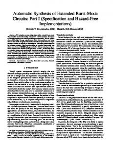
Figure 1.1: Synthesis at work for a simple Producer-Consumer problem

4

1.2. A Small Example

5

We first suppose that the actions involved in a trade between a producer and a consumer consist of the atomic actions of producing, sending, receiving, and consuming. So, first we fix the alphabet: Σ = {prod , send , rcv , cons}. Next, we specify a binary independence relation over the alphabet Σ: k ⊆ Σ × Σ. For instance, the independence relation is used to enforce that the actions of producing and consuming can and will be executed in parallel in the intended distributed implementation. A natural choice for our problem is to require that the following pairs of actions are independent: prod krcv , prod kcons, send kcons.

The complement with respect to Σ × Σ of the independence relation is called the dependence relation and is denoted by 6 k. Hence, we have 6 k = (Σ × Σ) \ k. The dependence relation is usually visualized using its associated dependence graph. The dependence graph is an undirected graph with the actions of Σ as vertices and the dependence relation 6 k as the edge relation. For our example, the dependence graph is: prod

cons

send

rcv

Since we want to synthesize a distributed system, we need to specify also a distribution pattern that our distributed implementation must comply with. More precisely, we give a set of names of processes (or agents), denoted by Proc, together with a local alphabet Σloc (p) ⊆ Σ associated to each process p ∈ Proc. Once we have an independence relation we can generate a distribution pattern such that two actions are independent if and only if there is no process containing both actions in his local alphabet. This can be achieved by choosing the local alphabets to be a covering by (maximal) cliques1 of the dependence graph. For our example, the only covering by cliques of the dependence graph is given by choosing one clique for each edge. This means, we have three processes Proc := {P1 , P2 , P3 } with the local alphabets Σloc (P1 ) := {prod , send }, Σloc (P2 ) := {send , rcv }, Σloc (P3 ) := {rcv , cons}.

The core of the synthesis problem is to associate a local (labeled) transition system to each process name such that the global synchronization on common actions of all the local transition systems is consistent with a given global behavior. For our example, we choose a global (regular) behavior as follows: Spec := Prefix(S1 ) ∩ Prefix(S2 ), where 1

A clique C of a graph G = (V, E) is by definition a subset of vertices C ⊆ V such that C × C ⊆ E.

6

Introduction

S1 = Shuffle((prod · send )∗ , (rcv · cons)∗ ), i.e., we allow the interleaving/shuffle of the behaviors of the ‘producer’ and ‘consumer’, S2 = (T ∗ · send · T ∗ · rcv · T ∗ )∗ , with T = Σ \ {send , rcv }, i.e., the consumer can only receive something that was previously sent, and Prefix (L) is a notation for the prefix-closure of the language L, i.e., the set of all the prefixes of the words of L. (We observe all the partial runs of the system.) The upper part of Figure 1.1 shows all the elements of the specification, i.e., the distribution pattern (top-left position) and the transition system exhibiting the global behavior1 described above (top-right position). The synthesis procedure will test whether the specification can be distributed and, if this is the case, will construct a distributed implementation (see also Figure 1.2). For simplicity, we choose as model of distributed implementation the synchronous products of transition systems [Arn94]. Informally, a synchronous product of transition systems over a given distribution consists of a set of local transition systems associated to each process which synchronize on common actions. For a given global specification, it is decidable to check whether there exists a synchronous product of transition systems accepting the same behavior as the global specification. The idea behind the distributability test is that of projection onto the local alphabets. More precisely, for each process p we construct a projection of the global specification onto the local alphabet Σloc (p) (that is, we ignore all the actions not in Σloc (p) by turning them into ε’s). Then, we have that the specification is distributable if and only if the synchronization on common actions of the projections is behaviorally equivalent to the specification. For our example, it turns out that the specification is indeed distributable. The projections of the specification onto the three local alphabets are depicted in the middle of Figure 1.1. It can be easily verified that their global synchronization on common actions has the same behavior as the given specification. The distributed implementation will then be the synchronous product of the three local component each of them having two local states. For instance, the run prod ·send ·rcv ·cons can be executed by the synchronous product in the following way: We start in the global initial state (0, 0, 0). First, P1 can locally execute a prod action and change its local state to 1, so the new global state is (1, 0, 0). Then, P1 and P2 can synchronize on the their send actions ( marked in the picture) changing in the same step their local states and we obtain (0, 1, 0). Similarly, P2 and P3 are both able to execute a rcv action, so they synchronize changing the global state to (0, 0, 1). Finally, P3 will locally execute a cons action, and by doing so, the distributed system returns to its initial global state (0, 0, 0). Once we have a distributed implementation, we can go further and translate the distributed transition system into other formalisms. At the bottom of Figure 1.1 we show such a possible translation that interprets P1 and P3 as two processes Producer and 1

Here by the behavior of a system we understand the set of all possible runs (sequences of consecutive actions) from the initial state of the system.

1.3. The Contribution of this Thesis

7

Specification Distribution and global behavior Roadmap TEST Is the specification distributable? no

yes

Heuristics Try to refine the specification so as to become distributable if possible

Synthesis Core algorithms + heuristics

Chapters 1, 2 Chapter 3 Chapter 4 Chapter 5 Chapter 6 Chapter 7

Distributed implementation Desired format

Figure 1.2: A diagrammatic flow of the synthesis approach followed in this thesis Consumer communicating via P2 which models a buffer of capacity 1 (the state 0 of

P2 reads ‘buffer empty’, while state 1 reads ‘buffer filled’; we assume that the buffer is initially empty). The Producer process will loop forever through the sequence of the following atomic actions: First it produces, then it waits for the buffer to be emptied (i.e., P2 moves to state 0). When the buffer is empty, the Producer will fill it (note that we abstracted away the information/material being traded between the Producer and the Consumer). On the opposite site, the Consumer will wait until the capacity 1 buffer is filled and only thereafter will empty it. Then, it will locally execute its ‘consume’ action.

1.3

The Contribution of this Thesis

The structure of the thesis follows the synthesis flow proposed in Figure 1.2. We discuss it below profiling some outcomes of our work: Chapter 2 We start with the prerequisites and some notations. Chapter 3 Then, we introduce the theoretical models (traces, asynchronous automata, synchronous products), together with various properties and characterizations used in the following chapters for the synthesis problem. Chapter 4 There exists the possibility that the given specification cannot be distributively implemented (this may be due to human error or incomplete specifications).

8

Introduction

The first major step is to check whether the two parts of the specification (the distribution and the global behavior) are consistent, i.e., test whether there exists indeed a distributed implementation for the given specification. We study this implementability test from computational complexity point of view and offer some heuristics to deal with the case when the test fails (i.e., we try to shape the initial global specification taking concurrency into account). Chapter 5 Assuming the implementability test is positive, the next step is the synthesis procedure itself. In some cases, checking the implementability of the specification may give a distributed implementation for free (e.g., for synchronous products). However, in other cases we have to go through the notoriously hard construction of Zielonka. Although we invested a great deal in trying to simplify this procedure, we managed to offer some alternatives only in some special cases. Chapter 6 We have prototype implementations for most of the algorithms proposed in the thesis. We used several heuristics that try to construct smaller asynchronous automata, which worked very well on the benchmarks used. In particular, we automatically synthesized new distributed algorithms for classical problems like mutual exclusion and dining philosophers. Chapter 7 We end the thesis with a short account on what was achieved and possible improvements. Publications Some of the results included in this thesis appeared already in the following papers: [S¸te02, S¸EM03, HS¸04, HS¸05].

⋄

I will not define time, space, place and motion, as being well known to all. Isaac Newton (Principia Mathematica)

Chapter 2 Preliminaries n this chapter, we present definitions and results frequently used in the rest of the thesis. Proofs will be sparsely given and those presented are there mainly for pedagogical reasons. For the missing proofs, the reader is referred to the cited papers. We start with basic notions and notations (from set, formal language, and graph theory) in Section 2.1. In Section 2.2 we introduce the classic concept of transition system and its accepting language together with some properties needed in the subsequent chapters. We present the finite automata as transition systems with a refined acceptance condition. The index at the end of the thesis will help at a later time to relocate the definitions and notations of this chapter.

I

2.1

Basic Notions and Notations

In this section we provide most of the basic notation conventions used throughout the thesis. We start with basic set theory. We continue with basic definitions on the algebraic structure of monoids. Then we introduce the basic concepts of formal languages over alphabets of actions used to generated words (alias executions) and languages (alias behaviors). We end with some graph theoretical concepts needed by the exposition.

2.1.1

Set Theory

When dealing with sets, we apply the following usual conventions taken from the classic set theory: The names for the sets start with a capital letter (A, B, C, . . .), while their elements with small letters (a, b, c, . . .). We use indices (a1 , a2 , a3 , . . .) or the prime symbol (a′ ) to distinguish between elements of the same type. The cardinality of a given set S, i.e., the number of distinct elements of S, is denoted by |S|. The operations on sets are respectively denoted as follows: 9

10

Preliminaries

– The empty set is denoted by ∅.

– The union of two sets is denoted by ∪.

– The intersection of two sets is denoted by ∩.

– The strict or proper inclusion of one set into another is denoted by ( .

– The cartesian product of two sets is denoted by ×. Given a set I of indices Q and a family (Si )i∈I of sets, the cartesian product of them is denoted by i∈I Si . – The difference of two sets is denoted by \. (By definition, A \ B := {x ∈ A | x 6∈ B}.)

– If we suppose that a set B is a subset of a set A, then the complement of B with respect to A is defined as A \ B and denoted by ∁B when A can be deduced from the context or directly A \ B, otherwise. – The power set of a set A, i.e., the set of all subsets of A, is denoted by – The set of all functions from a set A to a set B is denoted by B A .

P (A).

– A singleton is a set with only one element, X = {x}. To simplify notation, we may sometimes drop the braces around x. Given a class of sets C and an operation on sets O, we say that the class C is closed under operation O if and only if the result of the application of O to the elements of C is still in C. For example, the class of sets with at most 3 elements is closed under intersection, but not under union.

N

The set of natural numbers is denoted by . For two natural numbers i, j ∈ i ≤ j, we denote by [i..j] the set {k | i ≤ k ≤ j}.

N with

A (binary) relation is a set of pairs. If R is a relation and (a, b) is a pair in R, then we mostly write aRb. Suppose P is a set of properties of relations. The P-closure of a relation R is the smallest relation R′ that includes all the pairs of R and possesses the properties in P. For example, the transitive closure of R, denoted R+ , is defined by: 1) If (a, b) is in R, then (a, b) is in R+ . 2) If (a, b) is in R+ and (b, c) is in R, then (a, c) is in R+ . 3) Nothing is in R+ unless it so also follows from (1) and (2). An equivalence relation on a set S is a binary relation ∼⊆ S × S that satisfies the properties of reflexivity (∀a ∈ S : a ∼ a), symmetry (∀a, b ∈ S : a ∼ b ⇒ b ∼ a), and transitivity (∀a, b, c ∈ S : a ∼ b and b ∼ c ⇒ a ∼ c). For a set S and an equivalence ∼ on it, we have: – The equivalence class of an element a ∈ S is defined as {b ∈ S | b ∼ a} and denoted by [a]∼ .

2.1. Basic Notions and Notations

11

– The quotient set of S by ∼ is defined as the set of all equivalence classes of ∼, that is, {[a]∼ | a ∈ S} and is denoted by S/∼ .

– An equivalence ∼ on S is said to have finite index, if the quotient set S/∼ is finite. A partial order relation on a set S is a binary relation ⊑ on S that satisfies the properties of reflexivity (∀a ∈ S : a ⊑ a), antisymmetry (∀a, b ∈ S : a ⊑ b and b ⊑ a ⇒ a = b), and transitivity (∀a, b, c ∈ S : a ⊑ b and b ⊑ c ⇒ a ⊑ c).

A partially ordered set, alias poset, is a set equipped with a partial order relation.

2.1.2

Algebraic Notions

A monoid is a tuple (M, ·, 1), where M is a set, · is a associative binary operation, and 1 ∈ M is the identity element. (When confusion does not arise, we can use xy to indicate x · y.) A congruence relation ∼ over a monoid (M, ·, 1) is an equivalence over M that is compatible with the binary operation of the monoid, i.e., ∀x, y, x′ , y ′ ∈ M : x ∼ x′ and y ∼ y ′ ⇒ xy ∼ x′ y ′ . The quotient of a monoid (M, ·, 1) under a congruence ∼ is the monoid (M/∼ , ◦, [1]∼ ), where [x]∼ ◦[y]∼ := [x·y]∼ . (The fact that the equivalence ∼ is a congruence is used to prove that the given definition is well-defined.) A morphism φ from a monoid (M, ·M , 1M ) to another monoid (S, ·S , 1S ) is a function φ : M → S such that φ(1M ) = 1S and φ(x ·M y) = φ(x) ·S φ(y), for any x, y ∈ M . The surjective morphism [ ]∼ : M → M/∼ that associates to every element x ∈ M its equivalence class [x]∼ is called the canonical morphism. A subset X ⊆ M is closed under the congruence ∼ if and only if X is the union of some equivalence classes of ∼. Stated differently, X ⊆ M is closed under the congruence ∼ if and only if ∀x, y ∈ M : x ∈ X and x ∼ y ⇒ y ∈ X. A congruence ∼ is said to have finite index if the quotient M/∼ is a finite set.

2.1.3

Formal Languages

We describe the behavior of a sequential system by means of the classical theory of formal languages. The ingredients of this formalism are enumerated below: First of all, we have a non-empty finite set called the alphabet of actions, which we will usually denote by Σ. Then, we have the notion of a (finite) word or execution1 over Σ, which is a finite sequence of actions from the alphabet Σ. A word is represented by the concatenation of its actions. E.g., w = a1 a2 . . . an with ai ∈ Σ for all i ∈ [1..n]. The concatenation of two words will again be a word. Furthermore, we have: – We denote the concatenation of n copies of a word w ∈ Σ∗ as usually by wn .

– The length of a word w is denoted by |w|, i.e., if w = a1 a2 . . . an , then |w| = n. 1

In this thesis, we will not consider the case of infinite words/executions.

12

Preliminaries

– A special word is the empty word, denoted by ε, which is the word of length 0. – For w ∈ Σ∗ and a ∈ Σ, we denote by #a w the number of occurrences of the action a in the word w. For w ∈ Σ∗ , we denote by Σ(w) the alphabet of the word w, defined as the set of actions appearing in w, i.e., Σ(w) := {a ∈ Σ | #a w > 0}. Obviously, Σ(w) ⊆ Σ.

– For a word w ∈ Σ∗ and a subset S ⊆ Σ, we denote by w ↾S the projection of w onto S, which is obtained by erasing all actions in w which do not belong to S. Formally, for S ⊆ Σ, we define a function − ↾S : Σ → Σ such that a ↾S := ε if a 6∈ S and a ↾S := a if a ∈ S (we ‘erase’ the elements not belonging to S by replacing them with ε’s which are eventually absorbed). This function can be lifted to words − ↾S : Σ∗ → Σ∗ by the natural recursive definition: ε ↾S := ε and (xa) ↾S := x ↾S ·a ↾S for all x ∈ Σ∗ and a ∈ Σ.

– For two words t, u ∈ Σ∗ , we denote by Shuffle(t, u) the shuffle product of the two words t and u, which is the operation that constructs all the interleavings of all possible ‘cuttings’ of each of the two words. Formally, Shuffle(t, u) := {t1 u1 t2 u2 . . . tn un t = t1 . . . tn and u = u1 . . . un , where n ≥ 1 and ti , ui ∈ Σ∗ , ∀i ∈ [1..n]}. Diagrammatically, t = t1 · · · tk · · · tn u = u1 · · · uk · · · un

  

⇒ t1 u1 · · · tk uk · · · tn un ∈ Shuffle(t, u).

For example, we have Shuffle(ab, cd) = {abcd, acbd, acdb, cabd, cadb, cdab} and Shuffle(ab, a) = {aba, aab}. Note that in the above definition of Shuffle, ti , ui ∈ Σ∗ , which means they might even be ε. For instance, cdab ∈ Shuffle(ab, cd) by choosing k = 2, t1 = ε, t2 = ab, u1 = cd, and u2 = ε. – The word v ∈ Σ∗ is called a prefix of the word w ∈ Σ∗ if and only if there exists another word v ′ ∈ Σ∗ such that vv ′ = w. Dually, v ′ is called a suffix of w if and only if there exists v such that vv ′ = w. (Note that a word w is always a prefix of itself. Similarly, w is always the suffix of itself.) The set of all words over Σ is denoted by Σ∗ . In algebraic terms, the set Σ∗ together with the operation of word concatenation and the empty word ε form a monoid. In fact, Σ∗ is the free monoid generated by Σ. A set of words over Σ (i.e., a subset of Σ∗ ) is called a language over Σ. If we look at words as executions of a given system able to execute actions from an alphabet Σ, then a language over Σ can describe a behavior of the system. We can extend some of the operations on words to languages in the following way:


13

– For two languages L1 , L2 ⊆ Σ∗ , we define their concatenation as follows: L1 L2 := {w1 w2 | w1 ∈ L1 and w2 ∈ L2 }. For L ⊆ Σ∗ and a natural number n ≥ 1, we denote by Ln the concatenation of n copies of the language L. For n = 0, by definition we choose L0 := {ε}. Also, the union L1 ∪ L2 and intersection L1 ∩ L2 of the two languages L1 and L2 are defined as the union, respectively intersection operations on sets (of words). The complement of a language ∁L is defined as the complement with respect to Σ∗ , i.e., ∁L := Σ∗ \ L. Finally, we denote by L∗ the (Kleene) iteration of L which is defined as: [ L∗ := Ln . n≥0

– For L ⊆ Σ∗ , we denote by Σ(L) the alphabet of the language L, which is defined as the set of actions appearing in the words of L: [ Σ(L) := Σ(w). w∈L

Obviously, Σ(L) ⊆ Σ.

– For L ⊆ Σ∗ and a subset S ⊆ Σ, we denote by L ↾S the projection of L onto S, which is given by: L ↾S := {w ↾S | w ∈ L}.

– For L1 , L2 ⊆ Σ∗ , we denote by Shuffle(L1 , L2 ) the shuffle product of the languages L1 and L2 which is defined as: [ Shuffle(L1 , L2 ) := Shuffle(w1 , w2 ). w1 ∈L1 ,w2 ∈L2

– For L ⊆ Σ∗ , we denote by Prefix(L) the prefix-closure of L, which is the set of all prefixes of the words of L: Prefix(L) := {v ∈ Σ∗ | there exists w ∈ L such that v is a prefix of w}. A language L ⊆ Σ∗ is called prefix-closed if and only if L = Prefix(L). It is easy to see that a language is prefix-closed if and only if for any v, w ∈ Σ∗ , if w ∈ L and v is a prefix of w, then also v ∈ L. In particular, ε ∈ Prefix(L) for any language L. Moreover, the language Prefix(L) coincides with the smallest (w.r.t. set inclusion) prefix-closed language including L. Since we want to observe the behaviors of systems in all the intermediary steps, we will mainly work with prefix-closed languages, because they keep track of all the prefixes of each execution. The following proposition shows that the class of prefix-closed languages behaves well with respect to the operations introduced so far:

14

Preliminaries

Proposition 2.1 The class of prefix-closed languages over a given alphabet Σ is closed under the operations of union, intersection, concatenation, iteration, projection, shuffle product, and prefix-closure. The class of prefix-closed languages is not closed under complementation. Proof. For the union and intersection cases, the proof is obvious: If L1 , L2 ⊆ Σ∗ are two prefix-closed language, then both L1 ∪ L2 and L1 ∩ L2 are also prefix-closed. In fact, it is true that the union (respectively intersection) of an infinite number of prefix-closed languages is also prefix-closed. For the concatenation case, we show that for any two languages L1 , L2 ⊆ Σ∗ that are prefix-closed, we have that L1 L2 is also prefix-closed. Let w ∈ L1 L2 and v a prefix of w. From the fact that w ∈ L1 L2 , we have that there exist w1 ∈ L1 and w2 ∈ L2 such that w = w1 w2 . If v is a prefix of w, we have two cases: either v is a prefix of w1 or v = w1 v ′ with v ′ a prefix of w2 . In the first case, v ∈ L1 because w1 ∈ L1 and L1 is prefix-closed. Since L2 is prefix-closed, we have ε ∈ L2 . From v1 ∈ L1 , ε ∈ L2 , and the definition of the concatenation operation, we have indeed that v = vε ∈ L1 L2 . In the second case, since v ′ is a prefix of w2 ∈ L2 and L2 is prefix-closed, we have that v ′ ∈ L2 . From this fact and w1 ∈ L1 , we deduce that v = w1 v ′ ∈ L1 L2 . For the iteration case, we show that for any prefix-closed language L ∈ Σ∗ , we have that L∗ is also prefix-closed. We can first prove Ln is a prefix-closed language for any natural number n ≥ 0. The proof is by induction on n, using the fact that the class of prefix-closed is closed under concatenation. Using this, L∗ will be prefix-closed because the union of all the prefix-closed languages Ln with n ranging over is also prefix-closed (the class of prefix-closed languages is closed under (infinite) union). For the projection case, we show that for any prefix-closed language L ⊆ Σ∗ over Σ and any subset S of Σ, we have that L ↾S is also prefix-closed. Let w ∈ L ↾S and v a prefix of w. From w ∈ L ↾S , we have that there exists a word u ∈ L such that w = u ↾S (w is obtained from u by keeping only the action from S and removing all the others). Let a be the last action of v and k := #a (v) the number of the occurrences of a in v. We choose u′ to be the shortest prefix of u that contains exactly k occurrences of a. It is not difficult to show that v = u′ ↾S (using also the fact that w = u ↾S ). Since L is a prefix-closed language, u ∈ L, and u′ is a prefix of u, we have that u′ ∈ L, which implies that v ∈ L ↾S . For the shuffle product case, we show that for any two languages L1 , L2 ⊆ Σ∗ that are prefix-closed, we have that Shuffle(L1 , L2 ) is also prefix-closed. Let w ∈ Shuffle(L1 , L2 ) and v a prefix of w. From w ∈ Shuffle(L1 , L2 ), by definition, there exist t ∈ L1 and u ∈ L2 such that w ∈ Shuffle(t, u). Further, this means that there exist a natural number k ≥ 1 together with the words ti , ui ∈ Σ∗ for i ∈ [1..k] such that t = t1 . . . tk , u = u1 . . . uk , and w = t1 u1 . . . tk uk . By hypothesis, v is a prefix of w = t1 u1 . . . tk uk . Let j be the smallest index from [1..k] such that v is a prefix of t1 u1 . . . tj uj . This implies that v = t1 u1 . . . tj−1 uj−1 v0 , where v0 is a prefix of tj uj (just in case, we choose by definition t0 = u0 = ε). Performing an analysis similar to the concatenation case above, we can decompose v as v0t v0u such that v0t is a prefix of tj and v0u is a prefix of uj . This means that v = t1 u1 . . . tj−1 uj−1 v0t v0u , which further implies that v ∈ Shuffle(t1 . . . tj−1 v0t , u1 . . . uj−1 v0u ). Using the fact that L1 and L2 are prefix-closed in conjunction with property that v0t is a prefix of tj and v0u a prefix of uj , we conclude that v ∈ Shuffle(L1 , L2 ).

N


15

For the prefix-closure case, we must prove that if L ⊆ Σ∗ is a prefix-closed language, then Prefix(L) is also prefix-closed. But the very idea of the prefix-closure operation is to construct a prefix-closed language from a given language, in particular also from a prefixclosed one. Formally, it is easy to prove that the prefix-closure operation is idempotent, i.e., Prefix(Prefix(L)) = Prefix(L) for any language L, and, by definition, this means that Prefix(L) is prefix-closed for any L. For the complementation case, we can prove in fact that for any prefix-closed language L ⊆ Σ∗ , the complement of L is not prefix-closed anymore. More precisely, if L is a prefixclosed language, then ε ∈ L, which implies that ε 6∈ ∁L. But any prefix-closed language contains the empty word ε, which necessarily implies that ∁L is not prefix-closed. Regular Languages A ‘first-class citizen’ of the formal language theory is the class of regular languages (see for instance [HU79, Chapter 2]): Definition 2.2 (Regular language) The class of regular languages over an alphabet Σ is the smallest class containing the empty set ∅, the singleton languages {ε} and {a} for all a ∈ Σ, and being closed under the operations of union, concatenation, and Kleene iteration. The class of regular languages over Σ will be denoted by Reg(Σ). A language is called regular if it belongs to Reg(Σ). The regular languages can be represented by regular expressions. The latter show the order in which the three operations union, concatenation, and iteration are applied to the finite languages in order to obtain a given regular language. The regular expressions over an alphabet Σ and the languages they denote are recursively defined as follows: 1. ∅ is a regular expression and denotes the empty language. 2. ε is a regular expression and denotes the language {ε}. 3. For each a ∈ Σ, the symbol a is a regular expression and denotes the language {a}. 4. If r and s are regular expressions denoting the languages R and S, respectively, then (r + s), (r · s), and (r∗ ) are regular expressions that denote the languages R ∪ S, R · L, and R∗ , respectively.

In writing regular expression we can omit many parentheses if we assume that ∗ has the highest precedence and + the lowest. If we denote by L(r) the language of the regular expression r, then we have Reg(Σ) = {L(r) | r regular expression over Σ}. Example 2.3 In this thesis, we will mainly use regular languages for the specification of the global behavior of a system. For instance, the regular expression (send · rcv )∗ denotes a very simple communication pattern, where a message is sent (by a party), and then instantaneously received (by a peer party), this play may be repeating at leisure.

16

Preliminaries

Another classic characterization of regular languages is based on the notion of syntactic congruence: For a language L ⊆ Σ∗ , we denote by ∼L ⊆ Σ∗ × Σ∗ the syntactic congruence of L on Σ∗ , defined as follows: For v, w ∈ Σ∗ , v ∼L w if and only if ∀x, y ∈ Σ∗ : xvy ∈ L ⇔ xwy ∈ L. The characterization of regular languages based on the syntactic congruence is: Theorem 2.4 [Lal79, Chapter 6] A language L ⊆ Σ∗ is regular if and only if the syntactic congruence ∼L is of finite index. The following proposition recalls the property of the class of regular languages of being closed under all the language operations introduced so far: Proposition 2.5 The class of regular languages over a given alphabet Σ is closed under the operations of union, intersection, concatenation, iteration, complementation, projection, shuffle product, and prefix-closure. Proof. Proofs for the closure under the operations of union, intersection, concatenation, iteration, and complementation can be found for instance in [HU79, Section 3.2]. The projection − ↾S is a special case of homomorphism under which [HU79, Theorem 3.5] shows that the class of regular languages is closed. The closure of the class of regular languages under shuffle product is mentioned in [HU79, Exercise 6.6] (with the solution involving closure under homomorphisms and inverse homomorphisms of the class of regular languages). As far as the prefix-closure operation is concerned, if L ∈ Σ∗ is a regular language, it is easy to show that also Prefix(L) is regular. We know that L is regular if and only if there exists a finite-state automata A with a set of accepting states F such that L = L(A, F ) (see the notation of Definition 2.13). Then Prefix(L) = L(A, F ′ ), where F ′ is the set of all states of A. Hence, Prefix(L) is also regular. Let us denote by PrefReg(Σ) the class of prefix-closed regular languages over a given alphabet Σ. Then, from Propositions 2.1 and 2.5 we have the following closure result: Corollary 2.6 The class PrefReg(Σ) is closed under all the operations on languages introduced so far, except for the complementation operation.

2.1.4

Graph Theory

We recall here some concepts of graph theory used throughout the thesis. A graph G is a pair (V, E), where V is a finite set of vertices or nodes and E ⊆ V ×V is the set of edges or arcs. If E is symmetric, i.e., (x, y) ∈ E implies (y, x) ∈ E, then the graph is said to be undirected, otherwise it is directed.


17

f e

d a

b

c

Figure 2.1: Example of a graph [Pig93a] A subgraph G ′ of a graph G = (V, E) is a pair (V ′ , E ′ ) with V ′ ⊆ V and E ′ ⊆ E ∩ (V ′ × V ′ ).

The subgraph G ′ of G induced by a subset of vertices V ′ of V is the graph (V ′ , E ∩ (V ′ × V ′ )). A path from a node x to a node y in a graph G is a sequence (v0 , v1 , . . . , vn ) of vertices such that x = v0 , y = vn , and (vi−1 , vi ) ∈ E, for all i ∈ [1..n].

A cycle is a path with the initial and final node identical. A graph is called acyclic if it contains no cycles.

Two nodes x and y of a graph G are connected if there exists a path between them in G. A graph G is called connected if and only if every pair of its nodes is connected.

A connected component of a graph G is a maximal connected induced subgraph, i.e., a subgraph G ′ = (V ′ , E ′ ) with E ′ = E ∩ (V ′ × V ′ ) such that G ′ is connected and for every node a ∈ V \ V ′ the subgraph of G induced by V ′ ∪ {a} is not connected.

A tree is a graph in which any two nodes are connected by exactly one path. A spanning tree of a connected graph is a tree that includes every node of that graph. Two graphs G1 = (V1 , E1 ) and G2 = (V2 , E2 ) are isomorphic if there exists a bijection f : V1 → V2 between the sets of nodes that complies with the edge relations, i.e., (v, v ′ ) ∈ E1 if and only if (f (v), f (v ′ )) ∈ E2 . A clique of an undirected graph G = (V, E) is a subset V ′ of V that induces a complete graph, i.e., (x, y) ∈ E for all x, y ∈ V ′ with x 6= y. A clique V ′ of a graph G = (V, E) is maximal if every set V ′′ such that V ′ ( V ′′ ⊆ V is not a clique. S A clique cover of G is a family (V1 , . . . , Vn ) of cliques of G such V = ni=1 Vi and for every edge (x, y) ∈ E there exists an index i ∈ [1..n] such that (x, y) ∈ Vi .

For every undirected graph G = (V, E), there are two distinguished clique covers: 1. The clique cover consisting of cliques with at most two nodes. This cover contains the clique {x, y} for every pair of nodes x, y ∈ V such that (x, y) ∈ E, and the clique {x} for each isolated node x ∈ V , i.e., x is not connected to any other node from V .

18

Preliminaries

For the graph in Figure 2.1, this clique cover will consist of the sets: {a, b}, {a, d}, {b, c}, {b, d}, {b, e}, {d, e}, {d, f }, {e, f }. 2. The clique cover consisting of all the maximal cliques of G.

For the graph in Figure 2.1, this clique cover will consist of the sets: {a, b, d}, {d, b, e}, {e, b, c}, {d, e, f }.

Note that if we leave out the clique {d, b, e}, we still have a clique cover. This observation means that we do not necessarily need to consider the set of all maximal cliques in order to have a cover. In fact, it may be dangerous to consider the set of all maximal cliques as this set can be exponentially larger than the size of the graph: Take, for instance, G = (V, E), where V := {x1 , . . . , xn , y1 , . . . , yn } and E := V × V \ {{xi , yi } | i ∈ [1..n]}. Then, G has exactly 2n maximal cliques. On the other hand, the problem of finding a covering with a minimal number of cliques is NP-complete [GJ79].

Remark 2.7 If an undirected graph is transitive i.e., (x, y) ∈ E and (y, z) ∈ E implies (x, z) ∈ E, then the maximal cliques of G are disjoint and coincide with the connected components of G.

2.2

Transition Systems

One of the most general theoretical models able to capture (regular) behaviors of systems is that of transition system. A transition system consists of a number of states and a number of transitions between states which describe in each state which is the next possible state that the system can move to. Moreover, we have one or more initial states. Formally, we have the following definition: Definition 2.8 (Labeled transition system) A labeled transition system is a tuple TS = (Q, Σ, →, I), where Q is the set of states (Q is also called the state space) Σ is the alphabet of action labels, → is the transition relation, where → ⊆ Q × Σ × Q, and I is the (nonempty) set of initial states, where I ⊆ Q. Given a transition system TS = (Q, Σ, →, I), we have: TS is called finite, if the state space Q is finite. The size of TS is denoted by |TS | and is defined as the size of the state space |Σ|.

2.2. Transition Systems

19

a

If (q, a, q ′ ) ∈ →, we use the usual notation q −→ q ′ . Let w = w1 . . . wn be a word over Σ with wi ∈ Σ for all i ∈ [1..n]. For two states w q, q ′ , we write q −→ q ′ if there exist a path q0 , q1 , . . . , qn ∈ Q such that q = q0 , wi q ′ = qn , and qi−1 −→ qi for all i ∈ [1..n]. w

For two states q, q ′ ∈ Q, if there exist w ∈ Σ∗ such that q −→ q ′ , we say that q ′ is reachable from q, and dually, q is co-reachable from q ′ .

A transition system is called reachable if all the states are reachable from the set of initial states, that is, w

∀q ∈ Q ∃q0 ∈ I, w ∈ Σ∗ : q0 −→ q. For an equivalence relation ≡ ⊆ Q × Q over the states of TS , the quotient of TS over ≡ is defined as TS /≡ := (Q/≡ , Σ, →, I/≡ ), where Q/≡ , I/≡ are quotient sets a (cf. Section 2.1.1) and [q1 ]≡ −→ [q2 ]≡ if and only if there exist q1′ , q2′ ∈ Q such that a q1 ≡ q1′ , q2 ≡ q2′ , and q1′ −→ q2′ . Two transition systems TS 1 = (Q1 , Σ, →1 , I1 ) and TS 2 = (Q2 , Σ, →2 , I2 ) over the same alphabet of actions are isomorphic if there exists a bijection f : Q1 → Q2 between the state spaces that preserves the initial states and the transitions, i.e., f (I1 ) = I2 and (q, a, q ′ ) ∈ →1 if and only if (f (q), a, f (q ′ )) ∈ →2 . We denote by Σ(TS ) the alphabet of the transition system TS , defined as the set of actions labeling transitions of TS reachable from an initial state, i.e., w

a

Σ(TS ) := {a ∈ Σ | ∃q0 ∈ I, w ∈ Σ∗ , q, q ′ ∈ Q : q0 −→ q −→ q ′ }. Obviously, Σ(TS ) ⊆ Σ. TS is called deterministic, if a

a

|I| = 1 and ∀q, q ′ , q ′′ ∈ Q, a ∈ Σ : q −→ q ′ and q −→ q ′′ implies q ′ = q ′′ . TS is called acyclic, if the directed graph generated by the transition relation → is acyclic. Convention. Unless otherwise stated, when we say ‘transition system’, we mean ‘reachable finite labeled transition system’. We can use transition systems to express in a compact way behaviors of systems. Definition 2.9 (Run and language of a transition system) A run of TS is a word w ∈ Σ∗ that can be executed in TS starting in an initial state, i.e., w ∃q in ∈ I, q ∈ Q : q0 −→ q. The language of TS , denoted by L(TS ), is the set of all the runs of TS : w L(TS ) := {w ∈ Σ∗ | ∃q in ∈ I, q ∈ Q : q in −→ q}.

20

Preliminaries

roof 3

floor

wall 1

4 wall

floor

2

Figure 2.2: A house-like transition system Example 2.10 The language of the transition system in Figure 2.2 with 1 as the only initial state (marked by a short incoming arrow) is {ε, wall , floor , wall .floor , wall .roof , floor .wall }. Remark 2.11 For any transition system TS , we have Σ(TS ) = Σ(L(TS )), i.e., the alphabet of TS is equal to the alphabet of its language. Once we have two transition systems, we can compare their state spaces using the graph isomorphism or compare their languages. There are situations where the isomorphism is too strong and language equivalence too weak. An intermediate solution to this issue is given by the notion of bisimulation, which proved useful in the study of concurrent systems [Mil89]. Below we give a definition allowing multiple initial states: Definition 2.12 (Bisimulation) A (strong) bisimulation between a pair of transition systems TS 1 = (Q1 , Σ, →1 , I1 ) and TS 2 = (Q2 , Σ, →2 , I2 ) is a binary relation ∼ ⊆ Q1 × Q2 (for which we use the infix notation) such that: For each q1in ∈ I1 , there exists q2in ∈ I2 such that q1in ∼ q2in . For each q2in ∈ I2 , there exists q1in ∈ I1 such that q1in ∼ q2in . a

a

a

a

If q1 ∼ q2 and q1 −→1 q1′ , there exists q2′ such that q2 −→2 q2′ and q1′ ∼ q2′ . If q1 ∼ q2 and q2 −→2 q2′ , there exists q1′ such that q1 −→1 q1′ and q1′ ∼ q2′ . Having defined the bisimulation, for a transition system TS one can define ∼TS as the largest bisimulation between TS and itself. Since ∼TS defines an equivalence relation over the states of TS , we can construct the quotient of TS over ∼TS , denoted by TS /∼TS . Finite Automata A finer control over the behavior described by a transition system is obtained by specifying a set of accepting states. A run w will then be accepted only if the state of the transition system after executing w is accepting. Such an enriched transition system is called a finite automaton.


21

Definition 2.13 (Finite automaton) A finite automaton is a tuple A = (Q, Σ, →, I, F ), where (Q, Σ, →, I) is a transition system and F ⊆ Q is a set of accepting or final states. The language accepted by the automaton A with the set of accepting states F , denoted by L(A, F ) 1 , is defined as w

L(A, F ) := {w ∈ Σ∗ | ∃q in ∈ I, q fin ∈ F : q in −→ q fin }. As intended, finite automata are more expressive than the plain transition systems. The former are able to accept all the regular languages, while the latter only the strictly smaller class of prefix-closed regular languages. Theorem 2.14 (Kleene’s Theorem) For a fixed alphabet Σ, the class of languages accepted by finite automata coincides with the class of regular languages. Corollary 2.15 For a fixed alphabet Σ, the class of languages accepted by transition systems coincides with the class of prefix-closed regular languages. Proof. For one direction, we can see a transition system TS as a finite automaton with all states final. Then, by Theorem 2.14, L(TS ) is regular. L(TS ) is prefix-closed because any partial run of a run w ∈ L(TS ) is also a run of TS . For the reverse direction, let L ⊆ Σ∗ be a prefix-closed regular language. Since L is regular, by Theorem 2.14, there exists an automaton A = (Q, Σ, →, I, F ) such that L(A, F ) = L, where F ⊆ Q is the set of accepting states. Let Q′ ⊆ Q be the subset of states of A that are both reachable from an initial state and co-reachable from an accepting state. I.e., Q′ consists of the states that are on a path from an initial to an accepting state. We choose TS := (Q′ , Σ, →, I ′ ) as the transition system induced by Q′ and we show that L(TS ) = L(A, F ) (so L(TS ) = L). The inclusion L(A, F ) ⊆ L(TS ) follows easily from the fact that in particular the accepting states of Q are on a path from an initial to an accepting state in A (A is reachable). For the reverse inclusion, L(TS ) ⊆ L(A, F ), we use the hypothesis that w L = L(A, F ) is prefix-closed. Let w ∈ L(TS ). Then, there exists a path q in −→ q with q in ∈ I ′ and q ∈ Q′ in TS . By construction, the state q ∈ Q′ is on a path from an initial to an accepting state in A, so the word w is the prefix of a word of L(A, F ) and, since L(A, F ) is prefix-closed, this implies that w ∈ L(A, F ). Another classic result in automata theory shows that the deterministic restriction does not decrease the expressiveness power of finite automata. The same result will hold for transition systems. Theorem 2.16 For a fixed alphabet Σ, the class of languages accepted by finite automata coincides with the class of languages accepted by deterministic finite automata. Corollary 2.17 For a fixed alphabet Σ, the class of languages accepted by transition systems coincides with the class of languages accepted by deterministic transition systems. 1 We include the set of accepting states into the notation L(A, F ) for automata to stress the language acceptance condition difference to the transition systems (where all states are seen as accepting). In this thesis, we will mainly work with transition systems.

22

Preliminaries

Proof. Let L(TS ) be the language of a (nondeterministic) transition system TS . TS can be seen as a finite automaton with all states accepting. Then, we apply Theorem 2.16 (i.e., the usual subset construction) and we obtain a deterministic finite automaton A whose language is equal to L(TS ). Since L(TS ) is prefix-closed, we can apply the construction from the proof of Corollary 2.15 and obtain a deterministic transition system accepting L(TS ). An important property of deterministic finite automata regards minimization: Theorem 2.18 [HU79, Section 3.4] For each regular language L, there exists a unique (up to isomorphism) minimal deterministic finite automaton accepting L. Proof. (Construction idea – recalled here for further reference) For each regular language L, there exists a deterministic finite automaton A = (Q, Σ, →, {q0 }, F ) such that L = L(A, F ) (Theorems 2.14 and 2.16). Then, the minimal deterministic automaton accepting the same language as A is obtained by the classical minimization algorithm: 1. Remove the states unreachable from the (unique) initial state q0 .

2. Make the transition relation total, i.e., for any reachable state q ∈ Q and any action a a ∈ Σ, there exists q ′ ∈ Q such that q −→ q ′ . If the original transition relation was a not total, introduce a new non-final ‘sink state’ ⊥ such that: ⊥−→⊥ for any a ∈ Σ a a and q −→⊥ for each state q and action a such that there is no q ′ with q −→ q ′ . Once we know that → is deterministic and total, for each q ∈ Q and w ∈ Σ∗ , there w exists a unique state q ′ such that q −→ q ′ . We denote q ′ by δ(q, w).

3. Compute the following equivalence on the state space depending on the set of final states F : q ≈F q ′ if and only if (∀w ∈ Σ∗ : δ(q, w) ∈ F ⇔ δ(q ′ , w) ∈ F ) . 4. The minimal deterministic automaton is then obtained by taking the quotient w.r.t. ≈F .

The above constructed automaton is unique up to isomorphism w.r.t. the given properties. Corollary 2.19 For each prefix-closed regular language L, there exists a unique (up to isomorphism) minimal deterministic transition system accepting L.

Proof. (Construction idea) For each prefix-closed regular language L, there exists a deterministic transition system TS = (Q, Σ, →, {q0 }) accepting L (Corollaries 2.15 and 2.17). We can see TS as a finite automaton with all states final, i.e., F := Q and apply the minimization construction presented in the proof of Theorem 2.18. Given the special set of final states, computing the equivalence of step 3 in the minimization algorithm becomes: w ′ ∗ ′ w q ≈ q if and only if ∀w ∈ Σ : q −→⊥ ⇔ q −→⊥ . Additionally, at the end of the minimization procedure, we remove the sink state ⊥ (which was not final!) in order to obtain the minimal deterministic transition system TS ′ such that L = L(TS ′ ).


23

Finally, it is easy to see that imposing the acyclicity restriction to sequential machines, we obtain finite behaviors. (Note that a finite language is always regular.) Theorem 2.20 For a fixed alphabet Σ, the class of languages accepted by acyclic finite automata coincides with the class of finite languages. Corollary 2.21 For a fixed alphabet Σ, the class of languages accepted by acyclic transition systems coincides with the class of prefix-closed finite languages.

Discussion In this chapter we provided the basic ingredients needed in this thesis: set and graph theory, formal languages and sequential machines (transition systems and finite automata). We are now ready to move forward to learn about models of distributed systems which are introduced next.

⋄

A distributed system is one in which the failure of a computer you didn’t even know existed can render your own computer unusable. Leslie Lamport

Chapter 3 Distributed Transition Systems and the Synthesis Problem he synthesis problem for distributed systems we consider is: Given a global specification and a distribution structure, find if possible a distributed system complying with the specification. In this chapter, we present the models of distributed systems that we are working with together with characterization results that help solving the synthesis problem. The structure of the chapter is sketched below. We meet the first inhabitants of the theoretical world of concurrency in Section 3.1, where we get to know about independent actions and traces, which are classes of equivalent executions w.r.t. the independence relation. In Section 3.2, we move deeper into the concurrency area learning about distribution of actions over a set of processes and distributed transition systems. We present two related models of local transition systems synchronizing on common actions, namely the class of synchronous products of transition systems [Arn94] and of asynchronous automata [Zie87]. (The index at the end of the thesis will help at a later time to relocate the definitions and notations of this chapter.) Sections 3.3, respectively 3.4, give properties and characterizations of the global state space, respectively the languages, of the chosen models of distributed systems. Finally, Section 3.5 describes the versions of synthesis of distributed systems considered in this thesis.

T

3.1

Trace Theory

The theoretical interest for concurrent systems increased in the 60s with the seminal work of C.A. Petri [Pet62]. The new stream of fundamental research required appropriate tools to study the concurrent behaviors. The formal languages (Section 2.1.3) proved very suitable for sequential machines [HU79], but they showed their limitations when used within the new paradigm1 . At the end of the 70s, Mazurkiewicz [Maz77] introduced the notion 1 The most popular approach to study concurrent systems using classical formal languages theory was based on interleaving. In this case, true concurrency is replaced by the nondeterministic choice of the order of execution of a set of concurrent actions. Although useful in many situations, the interleaving unfortunately ‘forgets’ the concurrent structure of a computation which might be essential in problems

25

26

Distributed Transition Systems and the Synthesis Problem

roof wall

floor

Figure 3.1: The dependence graph of the concurrent alphabet of the house-like transition system of trace as a mathematical object able to maintain the information regarding the independence relation between the actions involved. Since then, the theory of traces continued to develop finding various applications (see surveys in [Maz87] and the monograph The Book of Traces [DR95]). In this section, we give the basics of trace theory. The first ingredient that we need is the notion of concurrent alphabet, which is simply an alphabet equipped with an independence relation between its actions: Definition 3.1 (Concurrent alphabet) A concurrent alphabet is a pair (Σ, k), where: Σ is a finite alphabet of actions and k ⊆ Σ × Σ is a symmetric and irreflexive binary relation called the independence or concurrency relation. The complementary relation of the independence relation is called the dependence relation and it is denoted by 6 k. Hence, by definition, 6 k := (Σ × Σ) \ k. Since k is symmetric and irreflexive, we have that 6 k is a symmetric and reflexive relation. Both the dependence and independence relations can be represented using undirected graphs. More precisely, the dependence graph associated to a concurrent alphabet is the undirected graph with vertex set Σ and with edge set 6 k \ {(a, a) | a ∈ Σ}. Dually, the independence graph of (Σ, k) is the undirected graph with vertex set Σ and with edge set k. Example 3.2 We can add a concurrency flavor to the house-like transition system of Figure 2.2 by supposing that the actions wall and floor are independent. So, we have the concurrent alphabet ( {wall , floor , roof }, {wall k floor } )

The dependence graph of the above concurrent alphabet is depicted in Figure 3.1.

We use the information provided by the independence relation so as to identify runs where adjacent independent actions are permuted. The intuition goes as follows: If two actions a and b are supposed to be independent (akb), then if at some point we can execute a followed by b, executing a should not affect in any way the possibility of executing b, so they may be executed in any order, in particular first b and then a. For instance, for Σ := {a, b, c} and akb, the runs caab, caba, and cbaa must be all equivalent. More precisely, we do not want to distinguish two runs that differ only in the order in which two adjacent independent actions are executed. This is theoretically implemented by constructing an equivalence relation in the following way: like system refinement or serializability of transactions in concurrent databases.

3.1. Trace Theory

27

Definition 3.3 (Trace equivalence) Given a concurrent alphabet (Σ, k), the trace equivalence ∼ over Σ∗ is defined as follows. For w, w′ ∈ Σ∗ , we have w ∼ w′ if and only if there exist the words v0 , . . . , vn ∈ Σ∗ such that w = v0 , w′ = vn , and for each i ∈ [1..n], there exist ui , u′i ∈ Σ∗ and ai , bi ∈ Σ such that ai kbi , vi−1 = ui ai bi u′i , and vi = ui bi ai u′i . Equivalently, the trace equivalence is the smallest equivalence ∼ on Σ∗ such that ∀u, v ∈ Σ∗ , a, b ∈ Σ : akb ⇒ uabv ∼ ubav. It is easy to see that the trace equivalence ∼ is in fact a congruence on Σ∗ with respect to concatenation, i.e., whenever w ∼ w′ , then for any words u, v ∈ Σ∗ , we have uwv ∼ uw′ v. Definition 3.4 (Trace monoid, trace, and trace language) Given a concurrent alphabet (Σ, k), the quotient of Σ∗ over the congruence ∼ is called the trace monoid and is usually denoted by (Σ, k).1 If we denote by [w] the ∼-equivalence class2 of the word w ∈ Σ∗ , then

M

M(Σ, k) = (Σ / , . , [ε]) ∗

∼

where ∀u, v ∈ Σ∗ : [u].[v] := [uv]. A trace is by definition an element of (Σ, k), that is, a ∼-equivalence class. A trace language is a subset of (Σ, k).

M

M

In case the independence (dependence) relation k has a special form, the trace monoid (Σ, k) allows special characterizations. For instance:

M

If k = ∅, then the trace monoid

M(Σ, k) is isomorphic to the free monoid Σ . ∗

If k is full, i.e., k = Σ × Σ \ {(a, a) | a ∈ Σ}, then w ∼ w′ if and only if #a w = #a w′ , for all a ∈ Σ. This implies that (Σ, k) is isomorphic to Σ .

M

N

If the dependence relation 6 k is transitive, then the maximal cliques Σ1 , . . . , Σn of the dependence graph are disjoint and (Σ, k) is isomorphic to the cartesian product Σ∗1 × . . . × Σ∗n of the free monoids generated by these cliques.

M

M

To every trace language T ⊆ (Σ, k), we can associate a (word) language of Σ∗ in the following way: lin(T ) := {w ∈ Σ∗ | ∃t ∈ T such that w ∈ t}.

For a trace language T , lin(T ) is a linearization3 function which generates the set of all members of each trace (read: equivalence class) of T . 1

M

The trace monoid (Σ, k) is also known in the literature as the free partially commutative monoid. We could have written the ∼-equivalence class as [w]∼ , but we did not what to unnecessarily burden the notation with the subscript ∼ , since in most contexts the ∼-equivalence will be implicit. 3 The name linearization comes from the fact that a trace is compactly described by a poset and the term linearization refers to the set of all linear (i.e., total) orders compatible with the poset. 2

28


Trace-closed Languages Since we are not mainly interested in studying the algebraic properties of trace languages, we will treat the trace languages as (word) languages of Σ∗ satisfying a closure condition rather than as subsets of the trace monoid (Σ, k). The closure property will of course depend on the equivalence relation ∼:

M

Definition 3.5 (Trace-closed language) Given a concurrent alphabet (Σ, k), we say that L ⊆ Σ∗ is a trace-closed language if it satisfies the following closure property: ∀w ∈ Σ∗ : w ∈ L ⇒ [w] ⊆ L. In other words, whenever w ∈ L and w ∼ w′ , then also w′ ∈ L. The following easy proposition shows that the classes of trace languages and traceclosed languages are isomorphic: Proposition 3.6 Given a concurrent alphabet (Σ, k), there is a 1–1 correspondence between the trace languages of (Σ, k) and the trace-closed languages over Σ∗ .

M

Proof. The 1–1 correspondence is given by the linearization function lin. For that, we show that:

M

lin is well-defined: For any T ⊆ (Σ, k), lin(T ) is a trace-closed language because if w ∈ lin(T ), then the trace t ∈ T such that w ∈ t is exactly [w], which will be necessarily included in lin(T ).

M

lin is injective: For T1 , T2 ⊆ (Σ, k) with T1 6= T2 , we show that lin(T1 ) 6= lin(T2 ). Without loss of generality, suppose there exists t ∈ T1 \ T2 . For w ∈ t, we have that w ∈ lin(T1 ). On the other hand, w 6∈ lin(T2 ), otherwise t ∈ T2 . So, w ∈ lin(T1 ) \ lin(T2 ), which means lin(T1 ) 6= lin(T2 ). lin is surjective: Let L ⊆ Σ∗ be a trace-closed language. We show that there exists a trace language T ⊆ (Σ, k) such that L = lin(T ). For T := {[w] | w ∈ L}, we have indeed that L = lin(T ): On one hand, L ⊆ lin(T ) because ∀w ∈ L : w ∈ [w] ⊆ lin(T ). On the other hand, lin(T ) ⊆ L because for any w ∈ lin(T ), there exists t = [w′ ] ∈ T with w′ ∈ L such that w ∈ [w′ ]. This implies w ∼ w′ and using the fact that L is trace-closed, we have that w ∈ L.

M

We mainly use languages to describe behaviors of systems. As we will later see, the behaviors of distributed systems are trace-closed, so it is good to know under which operations is the class of trace-closed languages closed. Proposition 3.7 The class of trace-closed languages over a concurrent alphabet (Σ, k) is closed under the operations of union, intersection, complementation, projection, shuffle product, and prefix-closure, but not closed under concatenation and iteration.

3.1. Trace Theory

29

 t = t1 · · · t′ .a · · · tn ∈ L1  u = u1 · · · b.u · · · un ∈ L2 ′

t = t1 · · · t

′

u = u1 · · · b

a · · · tn ∈ L1



u · · · un ∈ L2 ′

⇒ t1

  

u1 · · · t′ .a

b.u′ · · · tn

un ∈ Shuffle(L1 , L2 )

Splitting t′ .a and b.u′ , we manage to permute a and b using shuffle

⇒ t1

u 1 · · · t′

b

a

u ′ · · · tn

un ∈ Shuffle(L1 , L2 )

Figure 3.2: A detail in the proof of Proposition 3.7 Proof. The closure under union, intersection, complementation, projection, and prefixclosure can be easily proved. For the closure under shuffle product, the proof is a bit more elaborated. For every trace-closed languages L1 , L2 ⊆ Σ∗ , we must show that Shuffle(L1 , L2 ) is also trace-closed. Let w ∈ Shuffle(L1 , L2 ) and w′ ∼ w. By the definition of the trace equivalence, w′ is obtained from w by a number of permutations of adjacent independent actions. We prove that w′ ∈ Shuffle(L1 , L2 ) by induction on the number of permutations needed to obtain w′ from w. Base case : We assume that w′ is obtained from w by one permutation of the independent actions akb presumably appearing in a sequence ab in w. We show that w′ ∈ Shuffle(L1 , L2 ). By the definition of shuffle, there exist n ≥ 1 and ti , ui ∈ Σ∗ for i ∈ [1..n] such that t = t1 . . . tn ∈ L1 , u = u1 . . . un ∈ L2 , and w = t1 u1 . . . tn un ∈ Shuffle(t, u). We have to consider two cases depending on the position of the sequence ab in w = t1 u1 . . . tn un : Case 1 : ab appears inside a string tk , for a certain k ∈ [1..n]. Then, w′ = t1 u1 . . . t′k uk . . . tn un , where t′k is obtained from tk by replacing the chosen occurrence of ab by ba. Since t1 . . . tk . . . tn ∈ L1 and L1 is trace-closed, we have that t1 . . . t′k . . . tn ∈ L1 . So, w′ ∈ Shuffle(t1 . . . t′k . . . tn , u1 . . . uk . . . un ) ⊆ Shuffle(L1 , L2 ). Case 1’ : ab appears inside a string uk , for a certain k ∈ [1..n]. Similar to Case 1.

Case 2 : a appears as the last action of tk and b as the first action of uk , for a certain k ∈ [1..n]. Formally, there exist t′ , u′ ∈ Σ∗ such that tk = t′ a and uk = bu′ . In this case, w = t1 u1 . . . t′ abu′ . . . tn un and w′ = t1 u1 . . . t′ bau′ . . . tn un (a and b where permuted). To prove that w′ ∈ Shuffle(L1 , L2 ) we apply the trick depicted in Figure 3.2. More precisely, we refine the decomposition t1 . . . t′ a . . . tn of t, by considering t′ and a as separate substrings, i.e., we choose (t′i )i∈[1..n+1] such that t′i := ti for i ∈ [1..k − 1], t′k = t′ , t′k+1 = a, and t′i := ti−1 for i ∈ [k + 2..n]. Similarly, we split bu′ by choosing (u′i )i∈[1..n+1] such that u′i := ui for i ∈ [1..k − 1], u′k = b, u′k+1 = u′ , and u′i := ui−1 for i ∈ [k + 2..n].

30


Using the above decompositions of t and u, it is easy to see that w′ ∈ Shuffle(t, u) ⊆ Shuffle(L1 , L2 ) Case 2’ : a appears as the last action of uk and b as the first action of tk+1 , for a certain k ∈ [1 .. n − 1]. Similar to Case 2. Induction step : If we suppose w′ ∈ Shuffle(L1 , L2 ) for all w′ obtained from w by N permutations of adjacent independent actions, then it is immediate using the base case to show that the same property holds for N + 1. For the last part of the proposition, we show that the class of trace languages is not closed under concatenation and iteration: Take for instance, Σ = {a, b} with akb and the trace-closed languages L1 := {a}, L2 := {b}, and L := {ab, ba}. Then, L1 L2 = {ab} is not trace-closed, because ba 6∈ L1 L2 . Also, L∗ is not trace-closed, because abab ∈ L∗ , but aabb 6∈ L∗ . For a run w, the trace [w] consists of all words ∼-equivalent to w, which means that [w] is the closure of w with respect to the trace equivalence ∼. In a similar fashion, we can lift the trace-closure operation from words to languages in the natural way: For L ⊆ Σ∗ , we denote by [L] the trace-closure of the language L, which is defined as: [ [L] := [w]. w∈L

Equivalently, [L] is the smallest (w.r.t. set inclusion) trace-closed language including L. Regarding the classes of languages introduced as far, the trace-closure operator behaves as follows: Proposition 3.8 For a concurrent alphabet (Σ, k), neither the class of prefix-closed languages nor the class of regular languages is closed under the trace-closure operation. Proof. Counterexamples can be quickly given. Let the concurrent alphabet be ({a, b}, akb). On one hand, take the prefix-closed language L := {ǫ, a, ab}. Then, [L] is not trace-closed because ba ∈ [L], but b 6∈ [L]. On the other hand, take the regular language L := (ab)∗ . Then, [L] = {w ∈ Σ∗ | #a w = #b w}, which is a classical example of a non-regular language. Regular Trace Languages Maybe the most studied class of trace languages is that of regular trace languages. To introduce them, we follow the presentation and terminology of [Zie87]. There are other equivalent definitions and characterizations for the class of regular trace languages (which are sometimes known as recognizable trace languages), but since they do not play a rôle in this thesis we do not present them here (a curious reader is referred to [DR95]).

3.2. Distributed Transition Systems

31

Similar to the word languages, for a trace language T ⊆ syntactic congruence ∼T of T as follows: For t, t′ ∈ (Σ, k),

M

t ∼T t′ if and only if ∀x, y ∈

M(Σ, k), we define the

M(Σ, k) : xty ∈ T ⇔ xt y ∈ T. ′

Following [Zie87], we have the following definition (cf. Theorem 2.4): Definition 3.9 (Regular trace language) A trace language T ⊆ (Σ, k) is regular, if its associated syntactic congruence ∼T is of finite index. We denote the class of regular trace languages by eg(Σ, k).

M

R

The following two results relate the trace languages with their word counterparts: Lemma 3.10 [Zie87] Let T ⊆ v ∼lin(T ) w.

M(Σ, k) and v, w ∈ Σ . Then, [v] ∼ ∗

Proposition 3.11 [Zie87] For T ⊆ lin(T ) ∈ Reg(Σ).

T

[w] if and only if

M(Σ, k), we have T ∈ Reg(Σ, k) if and only if

From the above result and Proposition 3.6 we easily obtain: Corollary 3.12 Given a concurrent alphabet (Σ, k), there is a 1–1 correspondence between the regular trace languages of (Σ, k) and the regular trace-closed languages over Σ∗ .

M

For convenience, we will work more with trace-closed languages rather than with trace languages (we find it easier to work with classic languages of words than with languages of equivalence classes of words).

3.2

Distributed Transition Systems

In this section we generalize the notion of transition system to a distributed setting. A sequential system consists of one agent that executes a number of tasks in a certain order. Such a system can be theoretically modeled, for instance, by a transition system (see Definition 2.8). A distributed system consists of a number of agents that cooperate to execute a number of tasks. In real life, given the complexity of possible interactions, it is harder to find examples of sequential systems than of distributed ones. For instance, reading this piece of text by a human implies a mechanical synchronization of the two eyes (running over the lines) done in parallel with the synchronization of the hands (handling the cup of coffee/browsing the pages). A distributed system which has no interaction with the environment is called closed (e.g., a distributed algorithm processing a given input), otherwise it is called open (e.g., an operating system interacting with several users). In this thesis, we will only consider the case of closed distributed systems, so, unless otherwise specified, when we talk about a ‘distributed system’, we mean ‘closed distributed system’. Modeling a distributed system by an ordinary transition system is usually inefficient and ontologically inaccurate since the very paradigm of distributed activity is flattened

32


and thus structural information is lost. There is a number of already established theoretical models for distributed computation (Petri nets occupying a prominent position). In this thesis we will study two of them, both based on synchronization on common actions: the synchronous products of transition systems [Arn94] and the asynchronous automata [Zie87]. Loosely speaking, they consist of a number of local processes (or agents) that are able to execute a set of actions and which must synchronize on their common actions in order to change their local states. The latter model will take in consideration also the local states of the agents synchronizing to execute an action (so the latter model is more general than the former). Moreover, the synchronization on common actions requires a distribution pattern telling which agents are able to execute what actions. To exemplify the concepts, think of a building site with a team of diligent workers. We suppose that each worker has several specializations (e.g., masonry, carpentry, plumbing, plastering, painting). Due to their complexity, the tasks require the full manpower with a given specialization. Then, we can see the multitasking activity of building as a distributed transition system, where: the specializations are the possible actions, each task is the synchronization of workers, and each worker is a local process that takes part only in tasks involving his specializations. The next sections will introduce and discuss the notion of distribution of actions over a set of processes followed by the two notions of distributed transition systems which will be studied in this thesis.

3.2.1

Distributions

In this section we define the notion of distributed alphabet or (shorter) distribution. This will provide the ‘infrastructure’ of the distributed transition systems. Informally, a distributed alphabet consists of an alphabet of actions together with a set of processes and the information whether an action may be executed by a process or not. Formally, we have: Definition 3.13 (Distribution) A distribution is a tuple (Σ, Proc, ∆), where Σ is a nonempty, finite alphabet of actions, Proc is a nonempty, finite set of process labels, and ∆ ⊆ Σ × Proc is a binary relation between actions and processes such that each action is in relation with at least one process and vice versa, each process is in relation with at least one action1 . Once we have a distribution (Σ, Proc, ∆), we can extract action-oriented, respectively process-oriented information in the following way: For each action we can derive the (nonempty) set of processes that are able to execute that action. Namely, we have the function dom : Σ → P (Proc) \ ∅ defined for each a ∈ Σ as: dom(a) := {p ∈ Proc | (a, p) ∈ ∆}. 1

The two last conditions keep out abnormal specifications with ‘phantom’ actions or processes.


33

The function dom is called the domain function, as it provides the ‘domain’ where the action is active. One can give directly a domain function dom and from it to uniquely determine the distribution ∆ := {(a, p) | p ∈ dom(a)} that generates dom.1 Dually, for each process we can derive the (nonempty) set of actions that may be executed by that process. Namely, we have the function Σloc : Proc → P (Σ) \ ∅ defined for each p ∈ Proc as: Σloc (p) := {a ∈ Σ | (a, p) ∈ ∆}. The function Σloc provides the local alphabet of each process, i.e., the set of actions that the given process is able to execute. One can give directly the local alphabets by Σloc and from them to uniquely determine the distribution ∆ := {(a, p) | a ∈ Σloc (p)} that can generate them.2 Convention. In unequivocal contexts we will simply use ∆ to denote (Σ, Proc, ∆). Also, when it is more convenient, instead of the binary relation ∆, we provide the domain function or the local alphabets. According to the observations above, the distribution ∆ can be immediately recovered. Example 3.14 For the alphabet of the house-like transition system of Figure 2.2, Σ = {wall , floor , roof }, we can give a distribution over two processes/agents Proc = {1, 2} in the following way: ∆ := {(wall , 1), (roof , 1), (floor , 2), (roof , 2)}. If we interpret the set of processes as a team of two workers having various specializations, then the above distribution says that worker 1 can raise walls and roofs, while worker 2 is skilled to build floors and roofs. We can further generate the domains of the actions and the local alphabets of the processes: dom Σloc wall 1 1 wall , roof floor 2 2 floor , roof roof 1, 2 The Relation between Distributed and Concurrent Alphabets We have now two generalizations of the notion of alphabet of actions: the concurrent alphabet (Definition 3.1) and the distributed alphabet (Definition 3.13). The names themselves already hint at the difference between the two notions. The term ‘concurrent’ suggests that a concurrent alphabet (Σ, k) tells which actions can be executed in parallel, or concurrently. The term ‘distributed’ suggests that a distributed alphabet (Σ, Proc, ∆) 1

To comply with Definition 3.13, one has to check whether each process occurs in at least one domain. To comply with Definition 3.13, one has to check whether each action occurs in at least one local alphabet. 2

34


provides more information, namely, how the actions are dispersed in a network of local processes. Every distribution (Σ, Proc, ∆) gives rise to a natural independence relation k between the actions of Σ. For each pair a, b ∈ Σ we set: akb ⇔ dom(a) ∩ dom(b) = ∅. The intuition is that two actions are independent if and only if they are can be executed by disjoint sets of processes. With this definition, two independent actions cannot interfere in any way and thus they may be executed in parallel. Clearly, the relation defined above is irreflexive and symmetric. The other way around, for every concurrent alphabet (Σ, k), we can construct a distribution (Σ, Proc, ∆) such that the independence relation induced by ∆ is the same as k in the following way: 1. start with the dependence graph of (Σ, 6 k) 2. choose a clique cover of it 3. create a process pC for each clique C of the cover (so the size of Proc is equal to the size of the cover) 4. set (a, pC ) ∈ ∆ if and only if a belongs to the clique C. It is easy to show that indeed, the independence relation generated by the above distribution is equal to k. According to the observations in Section 2.1.4, there are several possibilities to choose a covering by cliques of a graph, and thus several distributions inducing the same independence relation. Special cases are the distributions generated by the covers of all maximal cliques and of cliques of at most two nodes (see page 17). Let us consider the concurrent alphabet of Example 3.2. The associated dependence graph (depicted in Figure 3.1) accepts the clique cover consisting of the two cliques {wall , roof } and {floor , roof }. According to the above algorithm, we create a process for each clique, say process 1, respectively process 2. Then the distribution obtained is exactly the one given in Example 3.14.

3.2.2

Synchronous Products of Transition Systems

We introduce now the first of our two models of distributed transition systems that we use in this thesis: the synchronous product of transition systems. Let us give the general idea on the structure and dynamics of a synchronous product of transition systems. As the name suggests, we have a number of local transition systems that synchronize to execute shared actions. The relation between the actions and the local transition systems is given by a distribution: We identify a process with each local transition system and the binary relation between actions and processes tells which actions can be executed by what local transition system. From this relation we extract the domains of the actions and the local alphabets of the local transition systems. Then, an


35

action a can be executed at a certain point by the synchronous product of the transition systems only if all the local transition systems of dom(a) are able to execute a at that point. The execution of a triggers the changing of the local states of the transition systems of dom(a) and leaves the rest of the local transition systems unaffected. The global state space of a synchronous product of transition systems is included in the cartesian product of the state spaces of the local transition systems. More precisely, the global state space consists of the global states that are reachable from a set of initial global states. Formally, we have the following definition: Definition 3.15 (Synchronous product of transition systems) A synchronous product of transition systems SP over a distribution (Σ, Proc, ∆) is a transition system (Q, Σ, →, I) for which there exist a family of local state sets (Qp )p∈Proc and a family of local transition relations (→p )p∈Proc with →p ⊆ Qp × Σloc (p) × Qp for each p ∈ Proc, such that: I⊆

Q

p∈Proc

Qp is the set of global initial states, and

Q Q ⊆ p∈Proc Qp consists of all the global states reachable from I by the following transition relation: a qp −→p qp′ for all p ∈ dom(a) and a ′ (qp )p∈Proc −→ (qp )p∈Proc ⇔ qp = qp′ for all p 6∈ dom(a). The synchronous product of transition systems SP is deterministic if the transition system (Q, Σ, →, I) is deterministic. The synchronous product of transition systems SP is acyclic if the transition system (Q, Σ, →, I) is acyclic. Sometimes, we simply use ‘synchronous product’ as a shorter version of the longer name ‘synchronous product of transition systems’. The synchronous product of transition systems is a popular model of distributed systems and can be found in the literature under different names like: mixed product [Dub86], product transition systems [TH98], loosely cooperating systems [Zie87, Muk02]. We see that the distribution (Σ, Proc, ∆) is deeply embedded in the above definition. We have one local state set together with a local transition relation for each process label. The local transitions are labeled with actions taken from the local alphabet of the process. Then, the synchronization on a common action affects only the processes of the domain of that action. Note that the transition systems are particular cases of synchronous products over distributions with |Proc| = 1. Definition 3.15 identifies a synchronous product of transition systems with the global transition system obtained from synchronizations on common actions (starting with a set of initial states). Nevertheless, this transition system can be generated using the local

36


The local transition systems

The synchronous product roof

roof (1, 0)

1 roof

wall 0

0

floor

floor

wall (0, 0)

1

(1, 1) wall

floor

(0, 1)

Figure 3.3: The synchronization of two workers state spaces (Qp )p∈Proc and (→p )p∈Proc , so an efficient data structure for synchronous products keeps only this local information and generates the needed part of the global transition system on demand. In this case, the size of a synchronous product is merely the sum of the sizes of the local transition relations. We use the global transition system in the first place of our definition just for the convenience of presentation. Example 3.16 Let us return to the paradigm of specialized workers given at the beginning of Section 3.2. We consider the distribution of Example 3.14 where we have two processes, alias two workers, that have as specializations the local alphabets {wall , roof } and {floor , roof }, respectively. To each worker we associate a behavior by two local states and two local transitions for each worker as shown on the left of Figure 3.3. More precisely, for the first worker we have wall

roof

floor

roof

Q1 := {0, 1} and {0 −→ 1, 1 −→ 1}, while for the second we have Q2 := {0, 1} and {0 −→ 1, 0 −→ 1}. The synchronous product of the two transition systems starting in the global initial state (0, 0) (so, I = {(0, 0)}) is given in the right of Figure 3.3. In the global state (0, 0) there are two actions executable: wall and floor . The action wall can be executed in (0, 0) because dom(wall ) = {1} and wall can be executed in local state 0 of the first component. In this case, only the first component will update to the wall local state 1. Thus, (0, 0) −→ (1, 0). A similar reasoning can be performed for the global floor

transition (0, 0) −→ (0, 1). The action roof has domain {1, 2}, so both workers must synchronize in order to execute it. That is, both of them must be in a local state where roof is enabled and they simultaneously change their local states by executing roof . In our case, roof can be roof executed only in the global state (1, 0) by the transition (1, 0) −→ (1, 1). We see that the resulted global transition system is isomorphic to the transition system of Example 2.10 (see Figure 2.2).


37

Q According to the Definition 3.15, Q ⊆ p∈Proc Qp , i.e., the global state space of a synchronous product is embedded in the cartesian product of its local state spaces (note that we consider in Q only the global Q states that are reachable from the initial states I). In the worst case, we have that Q = p∈Proc Qp , which implies that |Q| = ×p∈Proc |Qp |. This means that the size of the global state space may be exponentially (in the number of processes) larger than the size of local state spaces. This phenomenon is called the ‘state space explosion problem’ and is responsible for most difficulties in reasoning about distributed systems in practice. For instance, in the Example 3.16 above, we see that the global state space has size 4 which is the product of the sizes of the local state spaces. As a final notion of this section, by definition, the behavior of a synchronous product is given by the language that its global transition system accepts: Definition 3.17 (The language of a synchronous product of transition systems) The language accepted by the synchronous product of transition systems SP = (Q, Σ, → , I) is simply the language of its transition system: w

L(SP) := {w ∈ Σ∗ | ∃q in ∈ I, q ∈ Q : q in −→ q}. For the synchronous product of Example 3.16 (see Figure 3.3), the accepted language is: {ε, wall , floor , wall .floor , wall .roof , floor .wall }. A finer control over the accepted language is obtained adding a set of global final states F ⊆ Q and modifying the definition accordingly: w

L(SP, F ) := {w ∈ Σ∗ | ∃q in ∈ I, q fin ∈ F : q in −→ q fin }. Further details and discussions about the two versions above are postponed to Section 3.4.

3.2.3

Asynchronous Automata

We introduce now the second of our two models of distributed transition systems that we use in this thesis: the asynchronous automata [Zie87]. Compared to the synchronous products, the asynchronous automata are more complex and also more powerful: Any synchronous product can be presented as an asynchronous automaton and there are asynchronous automata that cannot be modeled by synchronous products. Based also on synchronization on common actions, the particularity of asynchronous automata is that the execution of an action depends on the local states of the processes taking part in the synchronization (i.e., the processes of the domain of the action). More precisely, we associate a transition relation with each action a which tells for which tuples of local states in dom(a), the action a can be executed and how the local states are modified. The local processes outside the domain are untouched. Formally, we have: Definition 3.18 (Asynchronous automaton) An asynchronous automaton AA over a distribution (Σ, Proc, ∆) is a transition system (Q, Σ, →, I) for which there exist

38


a family of local state sets (Qp )p∈Proc and a family of transition relations (→a )a∈Σ with →a ⊆ each a ∈ Σ,

Q

p∈dom(a)

Qp ×

Q

p∈dom(a)

Qp for

such that: I⊆

Q

p∈Proc

Qp is the set of global initial states, and

Q Q ⊆ p∈Proc Qp consists of all the global states reachable from I by the following transition relation: (qp )p∈dom(a) →a (qp′ )p∈dom(a) and a ′ (qp )p∈Proc −→ (qp )p∈Proc ⇔ qp = qp′ for all p 6∈ dom(a). The asynchronous automaton AA is deterministic if the transition system (Q, Σ, →, I) is deterministic. The asynchronous automaton AA is acyclic if the transition system (Q, Σ, →, I) is acyclic. The synchronization mechanism of asynchronous automata is more powerful than in the case of synchronous products. When synchronizing on a common action a, the processes of dom(a) update their local state taking into account the local states of their peers in dom(a). So, more information is exchanged via the relations →a (in the case of synchronous products, the processes agree on synchronization, but update their local states independently). The global transition system on the right of Figure 3.3 can be realized by an asynchronous automaton in the following way: The local state spaces associated with the two processes {1, 2} are the same as before Q1 = {0, 1} and Q2 = {0, 1}, and the local transition relations associated with the actions are: 0 →wall 1 in state space Q1 (because dom(wall ) = {1}), 0 →floor 1 in state space Q2 (because dom(floor ) = {2}), and (1, 0) →roof (1, 1) in state space Q1 × Q2 (because dom(roof ) = {1, 2}). In the global initial state (0, 0), we can execute wall and floor in parallel (since they affect disjoint sets of processes, i.e., the first, respectively second component). For instance, wall

roof

(0, 0) −→ (1, 0) because 0 →wall 1 and the first component of (0, 0) is 0. Then, (1, 0) −→ (1, 1) because (1, 0) →roof (1, 1). In the global state (1, 0) also floor can be executed because dom(floor ) = {2}, the second component of (1, 0) is 0, and 0 →floor 1, so we have floor

(1, 0) −→ (1, 1). On the other hand, wall cannot be executed in (1, 0) because the first component is 1 and there is no transition starting with 1 in →wall . In fact, it is not difficult to see that the synchronous products are weaker than the asynchronous automata:


39

roof (1, 0) wall (0, 0)

(1, 2)

roof

floor (2, 1)

(2, 2)

Figure 3.4: A ‘futuristic ambient’ asynchronous automaton that is not a synchronous product Remark 3.19 Every synchronous product over a distribution ∆ accepts a description as an asynchronous automaton over the same distribution ∆, but not the other way around. Proof. Let SP = (Q, Σ, →, I) be a synchronous product over distribution (Σ, Proc, ∆). Then, there exist a family of local state sets (Qp )p∈Proc and a family of local transition relations (→p )p∈Proc with →p ⊆ Qp ×Σloc (p)×Q ∈ Proc. We construct a family Q p for each p Q of transition relations (→a )a∈Σ with →a ⊆ p∈dom(a) Qp × p∈dom(a) Qp for each a ∈ Σ in the following way: a

(qp )p∈dom(a) →a (qp′ )p∈dom(a) ⇔ ∀p ∈ dom(a) : qp −→p qp′ . It is clear then that global transition system (Q, Σ, →, I) can be simulated by the synchronization specific to asynchronous automata: (qp )p∈dom(a) →a (qp′ )p∈dom(a) and a ′ (qp )p∈Proc −→ (qp )p∈Proc ⇔ qp = qp′ for all p 6∈ dom(a). On the other hand, consider again the distribution of Example 3.14 and the asynchronous automaton represented in Figure 3.4 obtained from the local state spaces Q1 = {0, 1, 2} and Q2 = {0, 1, 2}, and the local transition relations associated with the actions as:

(0, 0) →roof

0 →wall 1 in state space Q1 (dom(wall ) = {1}), 1 →floor 2 in state space Q2 (dom(floor ) = {2}), and (2, 1) and (1, 0) →roof (1, 2) in state space Q1 × Q2 (dom(roof ) = {1, 2}).

It is easy to see that the ‘modern architecture’ of Figure 3.4 is indeed the global transition system of the synchronization of the above transition relations. For instance, the only floor transition labeled with floor is (2, 1) −→ (2, 2) because (2, 1) is the only global reachable state (from (0, 0)) that has the second component 1 as required by 1 →floor 2. We prove now that the above transition system cannot be simulated by any synchronous product.1 By contradiction, suppose that such synchronous product exists. 1

An alternative proof can be given once we introduce characterizations of the global transition systems of synchronous products (see Theorem 3.26).

40


Then, there exist two workers (i.e., local processes) that synchronize to execute the roof

wall

given ‘architecture’ (i.e., global transition system). Since (0, 0) −→ (1, 0) −→ (1, 2) and Σloc (1) = {wall , roof }, the schedule of the first worker (i.e., the first local transiroof

f loor

tion relation) must include the sequence wall .roof . Since (0, 0) −→ (2, 1) −→ (2, 2) and Σloc (2) = {floor , roof }, the schedule of the second worker (i.e., the second local transition relation) must include the sequence roof .floor . Since the synchronization model is weaker than the one of asynchronous automata, the two workers only agree that they synchronize to construct a roof (dom(roof ) = {1, 2}) without exchanging any other information, so the following scenario is possible: The first worker rises a wall, then both workers team up (i.e., synchronize) to construct a roof, and at that point the second worker continues his schedule and builds a floor. The above will generate the sequence wall .roof .floor , which contradicts the original plan of the ‘building’ in Figure 3.4.

As a final notion of this section, by definition, the behavior of an asynchronous automaton is given by the language that its global transition system accepts: Definition 3.20 (The language of an asynchronous automaton) The language accepted by the asynchronous automaton AA = (Q, Σ, →, I) is simply the language of its transition system: w

L(AA) := {w ∈ Σ∗ | ∃q in ∈ I, q ∈ Q : q in −→ q}. A finer control over the accepted language is obtained adding a set of global final set F ⊆ Q and modifying the definition accordingly: w

L(AA, F ) := {w ∈ Σ∗ | ∃q in ∈ I, q fin ∈ F : q in −→ q fin }. In fact, Zielonka included a set of final states in the original definition of asynchronous automata [Zie87]. This refinement makes the model expressive enough that the class of languages accepted by asynchronous automata with final states coincides with the class of regular trace-closed languages. This solved the long-standing problem of finding a natural distributed model to exactly capture the regular trace-closed behaviors. Nonetheless, we will try to avoid a set of global final states for reasons given in Section 3.4.1.

3.3

Shapes

We know now that the distributed transition systems consist of local processes collaborating to execute actions. The first natural questions are: ‘What are the characteristics of the resulted global state space?’ and ‘Can we find a general pattern that allows us

3.3. Shapes

41

to recognize that a certain transition system originated from a distributed activity?’ In other words: What is the global ‘shape’ of a distributed transition system? In this section we examine structural properties of the global transition system of a distributed system and present characterizations for them from the literature. These characterizations provide theoretical bases for the synthesis of distributed transition systems (Section 3.5).

3.3.1

Diamonds et al.

A distributed system follows a distribution pattern. In turn, the distribution hides a natural independence relation between the actions (see end of Section 3.2.1), which can be uncovered considering the domains of the actions: akb ⇔ dom(a) ∩ dom(b) = ∅. Thus we obtain a concurrent alphabet (Σ, k) (Definition 3.1) telling which pairs of actions can be executed in parallel. We will see how this parallelism is reflected in our models of distributed transition systems. Looking at the Definitions 3.15 and 3.18, we notice that the synchronizations on common actions depend on the domain of the actions. Two independent actions have disjoint domains, which implies that the synchronizations on the two actions do not interfere. This means that in a certain global state the two actions may be executed in any order (cf. the trace equivalence in Definition 3.3). Moreover, if in a certain global state both actions are enabled, the execution of one of them does not hinder the execution of the other one. These two properties are formally captured by: Definition 3.21 (Independent and forward diamond properties) Let (Σ, k) be a concurrent alphabet and TS = (Q, Σ, →, I) a transition system. We say that TS satisfies the independent diamond (ID) and forward diamond (FD) properties if for any q1 , q2 , q3 ∈ Q and a, b ∈ Σ we have: a

b

b

a

ID : q1 −→ q2 −→ q3 ∧ akb ⇒ ∃q4 ∈ Q : q1 −→ q4 −→ q3 a

b

b

a

FD : q1 −→ q2 ∧ q1 −→ q3 ∧ akb ⇒ ∃q4 ∈ Q : q2 −→ q4 ∧ q3 −→ q4 . (Figure 3.5 presents the above properties graphically.) It is easy to see that every distributed transition system satisfies the ID and FD rules: Proposition 3.22 Let (Σ, Proc, ∆) be a distribution and k its corresponding independence relation. Then, every synchronous product SP = (Q, Σ, →, I) over ∆ satisfies the ID and FD properties. Similarly, every asynchronous automaton AA = (Q, Σ, →, I) over ∆ satisfies the ID and FD properties. Proof. It is enough to show that ID and FD hold for asynchronous automata because the same will hold for synchronous products using Remark 3.19. Let AA = (Q, Σ, →, I) be an asynchronous automaton over distribution (Σ, Proc, ∆) and q1 = (q1p )p∈Proc , q2 = (q2p )p∈Proc , and q3 = (q3p )p∈Proc be three global states of Q. Then, we have:

42


ID a

FD

1

a

akb

=⇒

2

1

b

2

4

a 2

1

b 3

a

akb

=⇒

2

b 3 a

b 3

1

b 3

b 4 a

Figure 3.5: The independent and forward diamond properties Formal description Σ := {a, b}, akb Q := {0, 1}, I := {0} a,b

Graphical description 0 a a

b

a,b

→ := { 0 −→ 1 −→ 0 }

b

1

Figure 3.6: A transition system satisfying ID and FD, but not isomorphic to an asynchronous automaton a

b

If q1 −→ q2 −→ q3 and akb, it is easy to see that the global state q4 = (q4p )p∈Proc given by: q4p := q3p for p ∈ dom(b) and q4p := q1p for p 6∈ dom(b), satisfies ID. a

b

If q1 −→ q2 , q1 −→ q3 , and akb, it is easy to see that the global state q4 = (q4p )p∈Proc given by: q4p := q2p for p ∈ dom(a) and q4p := q3p for p 6∈ dom(a), satisfies FD. Nevertheless, the ID and FD properties are not sufficient to characterize the shape of (the global transition systems of) distributed transition systems as the simple example below witnesses: Example 3.23 [Mor98] Let TS = (Q, Σ, →, I) be the transition system of Figure 3.6. It is easy to show that TS is the ‘smallest’ transition system such that TS satisfies ID and FD, but there is no asynchronous automaton isomorphic to it (and by Remark 3.19, also no synchronous product). Proof. Since it is obvious that TS satisfies ID and FD, we only have to prove that there is no asynchronous automaton isomorphic to it. By contradiction, suppose there exists such an asynchronous automaton whose distribution pattern is compliant with the given independence relation akb, i.e., dom(a) ∩ dom(b) = ∅. a From 0 −→ 1 and the definition of synchronization for asynchronous automata (Definition 3.18) we have that the local states of (the global states) 0 and 1 must be equal on b all processes of Proc \ dom(a). Similarly, from 0 −→ 1, the local states of 0 and 1 must be equal on all processes of Proc \ dom(b). Summing up, the local states of 0 and 1 coincide on all processes of (Proc \ dom(a)) ∪ (Proc \ dom(b)) = Proc \ (dom(a) ∩ dom(b)) = Proc, because dom(a)∩dom(b) = ∅. At this point we reached the contradiction that the distinct global states 0 and 1 have all the local states equal.

3.3. Shapes

43

Sometimes we can infer structural properties of the global transition relation from the local ones, as shown below. For synchronous products, we can lift the properties of being deterministic or acyclic from the local transition relations to the global generated one: Proposition 3.24 Let SP = (Q, Σ, →, I) be a synchronous product over a distribution (Σ, Proc, ∆) and let (→p )p∈Proc be its local transition relations (according to Definition 3.15). Then we have: 1. If all (→p )p∈Proc are deterministic1 , then their global synchronization → is also deterministic. 2. If all (→p )p∈Proc are acyclic, then their global synchronization → is also acyclic. 3. The converse implications of 1. and 2. above are not true in general. Proof. Easy: a

a

1. Let q = (qp )p∈Proc −→ q ′ = (qp′ )p∈Proc and q = (qp )p∈Proc −→ q ′′ (qp′′ )p∈Proc in →. a a Then, according to Definition 3.15, we have that qp −→ qp′ and qp −→ qp′′ for all p ∈ dom(a) (*) and qp′ = qp = qp′′ for all p 6∈ dom(a) (**). From (*) and the deterministic property of the local transition relations, we necessarily have that qp′ = qp′′ for all p ∈ dom(a), which together with (**) implies q ′ = q ′′ . a

a

an−1

a

n 1 2 2. By contradiction, suppose that → is contains the cycle q1 −→ q2 −→ . . . −→ qn −→ q1 (with n ≥ 1). Then, it not difficult to show that →p , where p ∈ dom(a1 ), contains a cycle (the projection on the component p of the global cycle). But this is a contradiction.

3. We choose the distribution of Σ := {a} over two processes Proc := {1, 2}, with dom(a) := {1, 2}. Also, for each process we choose the local state spaces Q1 := {q1 , q1′ } with →1 := {(q1 , a, q1 ), (q1 , a, q1′ )} and Q2 := {q2 } with →2 := ∅. If we take I := {(q1 , q2 )}, the global transition relation → is empty (because →2 = ∅), so → is both deterministic and acyclic. On the other hand, the first local transition →1 is neither deterministic, nor acyclic.

For asynchronous automata (which have a finer synchronization) the situation is slightly different than for synchronous products: Proposition 3.25 Let AA = (Q, Σ, →, I) be an asynchronous automaton over a distribution (Σ, Proc, ∆) and let (→a )a∈Σ be its local transition relations (according to Definition 3.18). Then we have: 1. If all (→a )a∈Σ are deterministic2 , then their global synchronization → is also deterministic1 . 1 A labeled transition relation →⊆ Q × Σ × Q is deterministic if and only if for all q, q ′ , q ′′ ∈ Q and a a a ∈ Σ such that q −→ q ′ and q −→ q ′′ , we necessarily have q ′ = q ′′ . 2 An unlabeled transition relation →⊆ S × S is deterministic if and only if for all s, s′ , s′′ ∈ S such that s → s′ and s → s′′ , we necessarily have s′ = s′′ .

44


2. If all (→a )a∈Σ are acyclic, then their global synchronization → is not necessarily acyclic. 3. If → is deterministic (respectively, acyclic), then not necessarily all (→a )a∈Σ are also deterministic (respectively, acyclic). Proof. Easy: a

a

1. Let q = (qp )p∈Proc −→ q ′ = (qp′ )p∈Proc and q = (qp )p∈Proc −→ (qp′′ )p∈Proc in →. Then, according to Definition 3.18, we have that (qp )p∈dom(a) →a (qp′ )p∈dom(a) and (qp )p∈dom(a) →a (qp′′ )p∈dom(a) (*), and qp′ = qp = qp′′ for all p 6∈ dom(a) (**). From (*) and the deterministic property of the local transition relations, we necessarily have that (qp′ )p∈dom(a) = (qp′′ )p∈dom(a) , which together with (**) implies q ′ = q ′′ . 2. Take for instance Σ = {a, b}, Proc = {1}, and dom(a) = dom(b) = 1. Also, take Q1 := {0, 1} with →a := {(0, 1)} and →b := {(1, 0)}. For I := {0}, we have Q = Q1 a b and →= {(0, a, 1), (1, b, 0)}. Then, → is cyclic (because 0 −→ 1 −→ 0), while the local transitions relations →a and →b are both acyclic. 3. In this case, the proof uses the fact in Definition 3.18 that the global state space is reachable and → is restricted to this part only:

We choose Σ := {a}, Proc := {1}, with dom(a) = {1}, and Q1 := {0, 1, 2} with →a := {(1, 1), (1, 2)}. If we take I := {0}, then Q := {0} and the global transition relation → is empty (because there is no s such that 0 →a s), so → is both deterministic and acyclic. On the other hand, the local transition relation →a is neither deterministic, nor acyclic.

Example 3.23 testifies that the ID and FD properties are not sufficient to characterize the shape of (the global transition systems of) distributed transition systems. Nevertheless, precise characterizations can be found in the literature [Mor98, CMT99, Mor99b, Muk02] and are presented in the following two sections (3.3.2 and 3.3.3).

3.3.2


We present a characterization theorem for the global transition system of synchronous products. More precisely, [CMT99, Muk02] give a set of three necessary and sufficient conditions that a transition system must satisfy in order to be isomorphic to a synchronous product over a given distribution. If such isomorphic synchronous product exists, then each of its local state spaces Qp (cf. Definition 3.15) is constructed as the quotient of the input state space under a local equivalence relation ≡p . These equivalences must be chosen such that the following hold: 1. an a-labeled transition does not affect the local states of the processes not contained in dom(a); 2. the global state space is no more than the cartesian product of the Qp ’s, and

3.3. Shapes

SP2

45

Last part of Definition 3.15 ... Q Q ⊆ p∈Proc Qp consists of all the global states reachable from I by the following transition relation: a qp −→p qp′ for all p ∈ dom(a) and a (qp )p∈Proc −→ (qp′ )p∈Proc ⇔ qp = qp′ for all p ∈ 6 dom(a).

SP3 SP1

Figure 3.7: The relation between conditions SP1 –SP3 and the definition of synchronous products 3. for an action a ∈ Σ, if the local states of the processes in dom(a) are able to perform an a-labeled transition, then a global synchronization must also be possible. Before we give the theorem, we need to introduce an abbreviation: Notation. For any two sets of indexes I and J such that J ⊆ I and an indexed family of binary relations (≡i )i∈I , the expression (q1 ≡J q2 ) abbreviates (∀j ∈ J : q1 ≡j q2 ). Theorem 3.26 [CMT99, Muk02] Let (Σ, Proc, ∆) be a distribution and TS = (Q, Σ, → , I)1 be a transition system. Then, the following are equivalent: (i) TS is isomorphic to a synchronous product of transition systems over ∆ (ii) For each p ∈ Proc, there exists an equivalence relation ≡p ⊆ Q × Q such that the following conditions hold (for any q1 , q2 ∈ Q and a ∈ Σ): a

SP1 : If q1 −→ q2 , then q1 ≡Proc\dom(a) q2 . SP2 : If q1 ≡Proc q2 , then q1 = q2 .

SP3 : Let a ∈ Σ and q ∈ Q. If for each p ∈ dom(a), there exist qp , qp′ ∈ Q such that a qp −→ qp′ and q ≡p qp , then for each choice of such qp ’s and qp′ ’s, there exists a q ′ ∈ Q such that q −→ q ′ and q ′ ≡p qp′ for each p ∈ dom(a).

Since the above theorem is not very easy to digest, we link in Figure 3.7 the definition of a synchronized product with the three conditions of Theorem 3.26 (see also the informal discussion preceding the theorem). Below we give an example that shows Theorem 3.26 ‘at work’: Example 3.27 Consider again the transition system of Figure 3.4 together with the distribution from Example 3.14, now with the austere look of Figure 3.8 (obtained by 1 In [CMT99, Muk02], Theorem 3.26 is restricted to the case when |I| = 1 (i.e., all transition systems have only one initial state). By inspecting the proof of [CMT99], it is easy to see that the theorem holds in fact for an arbitrary I. We also mention that in [CMT99, Muk02], the transition system TS is required to be reachable, but this is indeed the case in our framework: We assumed in Section 2.2 that all transition systems we work with are finite and reachable.

46


The distribution Σ := {a, b, c}, Proc := {1, 2} dom a {1} b {2} c {1, 2}

Transition system 0 a 1 c 2

c 3 b 4

Figure 3.8: An asynchronous automaton that is not a synchronous product relabeling wall by a, floor by b, and roof by c). In the proof of Remark 3.19, we gave intuitive arguments why the transition system is not (isomorphic to) a synchronous product. We can now provide an alternative formal proof using Theorem 3.26. By contradiction, suppose that the transition system of Figure 3.8 is isomorphic to a synchronous product over the distribution of Figure 3.8. Then, there exists a set of equivalences (≡p )p∈Proc such that SP1 –SP3 are satisfied and therefore we have: a

From SP1 applied to 0 −→ 1, we have that 0 ≡2 1 (recall that dom(a) = {1}, so Proc \ dom(a) = {2}). Next, we apply SP3 to the action c and the state q := 0 in the following way: For each process p of dom(c) = {1, 2}, we choose c

– for p = 1: 0 −→ 3 with 0 ≡1 0 (reflexivity of ≡1 ) and c

– for p = 2: 1 −→ 2 with 0 ≡2 1 (the application of SP1 above). c

Then, there exists necessarily q ′ such that 0 −→ q ′ and q ′ ≡1 3 and q ′ ≡2 2. Looking c at the transition relation, we see that the only q ′ such that 0 −→ q ′ is the state 3. So, we have 3 ≡1 3 and 3 ≡2 2 (*). Finally, we apply SP3 to the action b and the state 2. Since dom(b) = {2}, we b choose 3 −→ 4 for which we have 2 ≡2 3 (from (*) above). Then, there must exist b a q ′′ such that 2 −→ q ′′ and q ′′ ≡2 4. But there is no transition going out of state 2, so we reached a contradiction. Remark 3.28 At this point, we note that the characterization given by Theorem 3.26 is effective and constructive: effective, because we can always decide whether a transition system is isomorphic to a synchronous product or not (the number of all possible local equivalences is finite and we can test for each combination the SP1 –SP3 conditions) and

3.3. Shapes

47

constructive, because if there exists an isomorphic synchronous product, then we can derive its local transition systems by taking the quotients of the original transition system w.r.t. the local equivalences (see [CMT99, Muk02] for more details). The above remark solves what is called the synthesis problem for synchronous products modulo isomorphism (see Section 3.5) and whose computational complexity will be discussed in Chapter 4. In the special case of deterministic transition systems, Morin gave a similar characterization in [Mor98]. (In fact, the result for the deterministic case was published before the general case.) Theorem 3.29 [Mor98] Let (Σ, Proc, ∆) be a distribution and TS = (Q, Σ, →, {q in }) be a deterministic transition system. Then, we have: 1. There exists the least family of equivalences (≡p )p∈Proc over the states of Q such that the following conditions hold (for any q1 , q1′ , q2 , q2′ ∈ Q, a ∈ Σ, and p ∈ Proc): a

DSP1 : If q1 −→ q2 , then q1 ≡Proc\dom(a) q2 . a

a

DSP2 : If q1 −→ q1′ , q2 −→ q2′ , and q1 ≡p q2 , then q1′ ≡p q2′ .

2. The following are equivalent: (i) TS is isomorphic to a synchronous product of transition systems over ∆. (ii) For the equivalences (≡k )k∈Proc from 1. the following conditions hold: DSP3 : If q1 ≡Proc q2 , then q1 = q2 . DSP4 : Let a ∈ Σ and q ∈ Q. If for each p ∈ dom(a), there exist qp , qp′ ∈ Q a a such that qp −→ qp′ and q ≡p qp , then there exists q ′ ∈ Q such that q −→ q ′ . We note that SP1 , respectively SP2 are the same as DSP1 , respectively DSP3 . Moreover, for a deterministic transition system, SP3 is equivalent to DSP2 and DSP4 . Even if the conditions seem to be equivalent, the advantage of Theorem 3.29 over Theorem 3.26 is given by the elimination of the existential quantifier on the class of local equivalences. The first part of Theorem 3.29 constructs a set of equivalences (computed as a fixed point) which are further tested in the second part. This should give a more efficient implementation compared to the ‘guessing’ of local equivalences suggested by Theorem 3.26. The advantage of Theorem 3.29 over Theorem 3.26 is confirmed theoretically in Chapter 4 and practically in Chapter 6.

3.3.3


A characterization similar to Theorem 3.26 can be given for asynchronous automata: Theorem 3.30 [Mor99b, Muk02] Let (Σ, Proc, ∆) be a distribution and TS = (Q, Σ, → , I)1 be a transition system. Then, the following are equivalent: 1 We mention that in [Mor99b, Muk02], the transition system TS is required to be reachable, but this is indeed the case in our framework: We assumed in Section 2.2 that all transition systems we work with are finite and reachable.

48


(i) TS is isomorphic to an asynchronous automaton over ∆ (ii) For each p ∈ Proc, there exists an equivalence relation ≡p ⊆ Q × Q such that the following conditions hold (for any q1 , q2 ∈ Q and a ∈ Σ): a

AA1 : If q1 −→ q2 , then q1 ≡Proc\dom(a) q2 . AA2 : If q1 ≡Proc q2 , then q1 = q2 .

a

a

AA3 : If q1 −→ q1′ and q1 ≡dom(a) q2 , then there exists q2′ ∈ Q such that q2 −→ q2′ and q2′ ≡dom(a) q1′ .

Since SP1 , respectively SP2 , is the same as AA1 , respectively AA2 , the difference between Theorem 3.26 and Theorem 3.30 is given by SP3 vs. AA3 . More precisely, it is easy to see that SP3 implies AA3 . This observation gives an alternative proof to Remark 3.19 saying that any synchronous product accepts a description as an asynchronous automaton. As a simple (pedagogical) exercise, we show how Theorem 3.30 can be used to prove structural properties of distributed transition systems: Remark 3.31 Let (Σ, Proc, ∆) be a distribution and TS = (Q, Σ, →, I) be (the global transition system of) an asynchronous automata. Then: 1. TS satisfies ID and FD (Proposition 3.22). a,b

2. There exist no q, q ′ ∈ Q, a, b ∈ Σ such that q −→ q ′ , q 6= q ′ , and akb.

As a consequence, Example 3.23 cannot be an asynchronous automata (because a,b

0 −→ 1 and akb). Proof. Easy: 1. We use Theorem 3.30 to give an alternative proof to Proposition 3.22. We consider only the FD case (ID being similar). a

b

b

For q1 −→ q2 , q1 −→ q3 , and akb, we show that there exists q4 such that q2 −→ q4 a and q3 −→ q4 (cf. Figure 3.5). Since TS is an asynchronous automaton over ∆, according to Theorem 3.30, there must exist a family of local equivalences (≡p )p∈Proc satisfying AA1 –AA3 . We apply the three conditions in turn as follows: a

From AA1 applied to q1 −→ q2 , we have q1 ≡Proc\dom(a) q2 and from akb, by definition, we have dom(a) ∩ dom(b) = ∅, which is equivalent to dom(b) ⊆ (Proc \ dom(a)). Thus, we have q1 ≡dom(b) q2 . b

From AA1 applied to q1 −→ q3 , we similarly obtain q1 ≡dom(a) q3 . b

From AA3 applied to q1 −→ q3 and q1 ≡dom(b) q2 , there exists q4′ such that b

q2 −→ q4′ and q4′ ≡dom(b) q3 . Moreover, we have that q4′ ≡Proc\dom(a) q3 (*): If p ∈ (Proc \ dom(a)) \ dom(b), then q4′ ≡p q3 from transitivity applied to q4′ ≡p q2 , q2 ≡p q1 , and q1 ≡p q3 (the last three equivalences are obtained b a b applying AA1 to q2 −→ q4′ , q1 −→ q2 , respectively q1 −→ q3 ).

3.3. Shapes

49

a

From AA3 applied to q1 −→ q2 and q1 ≡dom(a) q3 , there exists q4′′ such that a a q3 −→ q4′′ and q4′′ ≡dom(a) q2 . From AA1 applied to q3 −→ q4′′ , we have that q3 ≡Proc\dom(a) q4′′ , which together with (*) gives (by transitivity) that q4′ ≡Proc\dom(a) q4′′ . Similarly, we have also q4′ ≡Proc\dom(b) q4′′ . From the last two equivalences and dom(a) ∩ dom(b) = ∅, we have that q4′ ≡Proc q4′′ . Finally, from AA2 applied to q4′ ≡Proc q4′′ , we have that q4′ = q4′′ and we denote a this single state by q4 . Then, this state q4 satisfies condition FD for q1 −→ q2 , b q1 −→ q3 , and akb [q.e.d.]. a,b

2. By contradiction, assume there exist q 6= q ′ such that q −→ q ′ and akb. Applying a b AA1 to q1 −→ q2 , respectively q1 −→ q2 we easily obtain that q1 ≡Proc q2 , which by AA2 implies that q1 = q2 , which is a contradiction. For deterministic transition systems, a characterization similar to Theorem 3.29 is available also for asynchronous automata: Theorem 3.32 [Mor98] Let (Σ, Proc, ∆) be a distribution and TS = (Q, Σ, →, {q in }) be a deterministic transition system. Then, we have: 1. There exists the least family of equivalences (≡p )p∈Proc over the states of Q such that the following conditions hold (for any q1 , q1′ , q2 , q2′ ∈ Q, a ∈ Σ, and p ∈ Proc): a

DAA1 : If q1 −→ q2 , then q1 ≡Proc\dom(a) q2 . a

a

DAA2 : If q1 −→ q1′ , q2 −→ q2′ , and q1 ≡dom(a) q2 , then q1′ ≡dom(a) q2′ . 2. The following are equivalent: (i) TS is isomorphic to an asynchronous automaton over ∆. (ii) For the equivalences (≡k )k∈Proc from 1. the following conditions hold: DAA3 : If q1 ≡Proc q2 , then q1 = q2 . a DAA4 : If q1 −→ q1′ and q1 ≡dom(a) q2 , then there exists q2′ ∈ Q such that a q2 −→ q2′ . We end with a ‘genealogical’ remark. The results of Sections 3.3.2 and 3.3.3 have their roots in the theory of regions [ER90], proposed by Ehrenfeucht and Rozenberg in the early 90s to characterize (modulo isomorphism) the reachability graphs of Petri nets1 . The connection between the Theorems 3.26, 3.30 and the theory of regions is given by the fact that the synchronous products and the asynchronous automata can be seen as particular cases of (1-safe) Petri nets. 1

Loosely speaking, a region is a subset of states that is consistently entered, respectively exited by transitions having the same label.

50

3.4


Languages

In this section we study the languages accepted by our two models of distributed systems. We start with a short discussion regarding the final states of a distributed system. Then, we show the relation between the structural diamond properties of transition systems and closure properties of their accepted languages. We continue the presentation with characterizations of the languages of distributed transition systems with remarks about special cases. We finish with an expressiveness comparison of various classes of languages. Before we start, we introduce notations for the classes of languages accepted by distributed transition systems with different constraints. Notation. Let us fix a distribution (Σ, Proc, ∆). Then, for each of the theoretical models M below: NSP DSP NAA DAA

nondeterministic synchronous products, deterministic synchronous products, nondeterministic asynchronous automata, and deterministic asynchronous automata,

we denote by L(M ), respectively L(M, F ) the class of languages accepted by the model M over ∆ without, respectively with a set of final states. Moreover, we consider also acyclic versions of the above four classes of systems, and the notation is obtained by adding the prefix ‘A’. So, we have ANSP ADSP ANAA ADAA

acyclic acyclic acyclic acyclic

nondeterministic synchronous products, deterministic synchronous products, nondeterministic asynchronous automata, and deterministic asynchronous automata,

For instance, L(DAA, F ) denotes the class of all languages L = L(AA, F ) where AA is a deterministic asynchronous automaton over ∆ with a set of final states F , while L(AN SP ) denotes the class of all languages L = L(SP) where SP is an acyclic (nondeterministic) synchronous product over ∆. A small clarification: As in classic automata theory, when we use the term ‘nondeterministic’ for a (distributed) transition system, we do not mean a system that is ‘not deterministic’ (thus excluding the deterministic systems from the class), but we mean a general transition system that may as well be deterministic or not. According to Definitions 3.15 and 3.18, the usage of the descriptive adjective ‘nondeterministic’ is redundant, but may help to better differentiate various classes of models.

3.4. Languages

3.4.1

51

Final States

In this subsection we shortly discuss the appropriateness of final/accepting states to distributed systems. The behavior or the language of a system is given by the set of all its possible runs. A run has a starting point and an ending point. Therefore, we can ‘tune’ the language of a system by appropriately modifying the set of initial and final states. This works per se for sequential machines (Definition 2.13) and we could naturally extend the idea to distributed transition systems and choose a set of initial and final global states. This is a seamless theoretical approach, as one could simply observe the global transition system of a distributed system as a sequential system and apply the classic reasoning. Yet, there is a pragmatic objection to the above choice of global final states: An implementation of the mechanism of telling when we can accept a run implies the existence of a global controller that has access to all the local states and decides whether their tuple is accepting (i.e., final) or not. However, this is against the guiding principle that a distributed system involves only local synchronization. Also, it is unnatural to have a set of final global states that declare a posteriori that a run already executed is not valid because the reached global state is not final (the processes have only partial views and therefore cannot prevent possible executions that do not satisfy a global condition). Therefore: In this thesis we will not to deal with final states and will observe all the possible executions of the distributed transition systems (see L(SP), respectively L(AA) in Definitions 3.17, respectively 3.20). In other words, we consider by default all the reachable global states as accepting. We mention two other related models that address the above mentioned problems regarding a set of global final states for asynchronous automata. In his paper [Zie89], Zielonka restricts the model of asynchronous automata with final states to those having the following safety property: from any global state reachable from an initial state, we can always reach a final state. The new class, called safe asynchronous automata, was shown to have the same expressive power as the asynchronous automata with final states, but only in case we allow nondeterminism. Another possibility, mentioned by Pighizzini in [Pig93a, Section 3.3], is to have a set of local final states for each process of the distribution and to consider the cartesian product of the sets of local final states as the set of global final states. We will further discuss these options at a later time.

3.4.2

Traces of Diamonds

In Section 3.3.1, we have seen how the independence relation between actions ‘watermarks’ the structures of distributed systems. In this section, we study the ‘reflexions’ of the independence relation in the languages of distributed transition systems and show the relation of these languages to the trace languages from Section 3.1. In Section 3.3.1, the ID and FD diamond properties were shown to hold for the class of distributed systems over a concurrent alphabet (Σ, k). Since the behavior of a system depends of course on its shape, it is natural to investigate the properties of the languages of systems satisfying the diamond properties. Thus, it is easy to see that to ID it corresponds

52


the trace-closure property (Definition 3.5): For all w, w′ ∈ Σ∗ , and a, b ∈ Σ, it holds wabw′ ∈ L ∧ akb ⇒ wbaw′ ∈ L. On the other hand, to FD we can associate a notion of forward closure1 : Definition 3.33 (Forward-closed language) Let (Σ, k) be a concurrent alphabet. A language L ⊆ Σ∗ is called forward-closed if for all w ∈ Σ∗ , and a, b ∈ Σ it holds: wa ∈ L ∧ wb ∈ L ∧ akb ⇒ wab ∈ L. The following proposition confirms the relation between the above structural and language properties: Proposition 3.34 For any concurrent alphabet (Σ, k) and any transition system TS = (Q, Σ, →, I), we have: 1. If TS satisfies ID, then L(TS ) is trace-closed. 2. If TS is deterministic and satisfies FD, then L(TS ) is forward-closed. 3. If TS is nondeterministic and satisfies FD, then it is not always the case that L(TS ) is forward-closed. Proof.

1. Let w, w′ ∈ Σ∗ and a, b ∈ Σ such that wabw′ ∈ L(TS ) and akb. Then, there w

a

b

w′

a

exist q in ∈ I, q1 , q2 , q3 ∈ Q such that q in −→ q1 −→ q2 −→ q3 −→ q4 . From q1 −→ a b b q2 −→ q3 and akb, by ID we have that there exists q2′ such that q1 −→ q2′ −→ q3 . So w

b

a

w′

q in −→ q1 −→ q2′ −→ q3 −→ q4 , which implies that wbaw′ ∈ L(TS ).

2. Let w ∈ Σ∗ and a, b ∈ Σ such that wa, wb ∈ L(TS ) and akb. Since TS is deterministic, there exists a unique initial state q in and unique states q1 , q2 , q3 ∈ Q such w a b a b that q in −→ q1 , q1 −→ q2 , and q1 −→ q3 . From q1 −→ q2 , q1 −→ q3 , and akb, b a by FD we have that there exists q4 ∈ Q such that q2 −→ q4 and q3 −→ q4 . So w a b q in −→ q1 −→ q2 −→ q4 in TS , which implies that wab ∈ L(TS ). 3. For the concurrent alphabet Σ := {a, b, c} with akb, the nondeterministic transition systems of Figure 3.9 satisfy FD (and ID). On the other hand, the language accepted by the left, respectively right, transition system, are {ε, a, b}, respectively {ε, c, ca, cb}. We see that none of the two languages above is forward-closed (E.g., for the second language we have that akb and ca, cb belong to the language, but cab does not belong to it.) The left transition system has multiple initial states, while the second one has only one initial state (but nondeterministic choice for c). 1

This property bears other different names like: properness in [Maz87] (see also [DR95, Chapter 9]), fI-closure in [Muk02], coherence in [BM03], or safe-branching in [S ¸ EM03].

3.4. Languages

Independence Σ := {a, b, c} with akb

53

First transition system

Second transition system 0

1

c

2

a

c

1 a

b 3

2 b 4

3

Figure 3.9: Two transition systems satisfying FD whose languages are not forward-closed Since the distributed transition systems satisfy the ID and FD properties (cf. Proposition 3.22), we further obtain: Corollary 3.35 Let (Σ, Proc, ∆) be a distribution and k its corresponding independence relation. Then: 1. L(DSP ), L(DAA), L(ADSP ), and L(ADAA) are included in the class of forwardclosed trace-closed languages. 2. L(N SP ), L(N AA), L(AN SP ), and L(AN AA) are included in the class of traceclosed languages. We can investigate also the structural properties of regular languages satisfying the forward and trace closure properties. Interestingly enough, we recover the ID and FD properties, but only for the minimal transition system accepting the given language1 . The following result will later be useful in the distributed implementability test. Proposition 3.36 Let (Σ, k) be a concurrent alphabet and L ⊆ Σ∗ a prefix-closed regular language. Then, the following are equivalent: 1. L is forward- and trace-closed. 2. The minimal deterministic transition system accepting L satisfies ID and FD. Proof. First of all, according to Corollary 2.19, for the prefix-closed regular language L, there exists a unique (up to isomorphism) minimal deterministic transition system, say TS = (Q, Σ, →, {q in }), such that L = L(TS ). 1 ⇒ 2 : Let us first prove that TS satisfies ID. Let q1 , q2 , q3 ∈ Q and akb such that w0 a b q1 −→ q2 −→ q3 . Since TS is reachable, there exists w0 ∈ Σ∗ such that q in −→ q1 . So, w0 ab ∈ L(TS ). Since L(TS ) is trace-closed, we have that also w0 ba ∈ L(TS ), w0 b a which implies that there exists two states q4 , q4′ ∈ Q such that q in −→ q1 −→ q4 −→ 1

According to Proposition 3.34, if a deterministic transition system satisfies FD, then its language is forward-closed, but not the other way around: E.g., the language L := {ε, a, b, ab, ba} is forward-closed b

a

b

a

for akb, but the (non-minimal) deterministic transition system 2 ←− 1 ←− 0 −→ 3 −→ 4 (with 0 initial state) accepts L and does not satisfy FD.

54


q4′ (after executing w0 from q in , we always reach q1 , because TS is deterministic). If we prove that q3 is equal to q4′ , we can conclude that the ‘diamond’ property ID holds in q1 for akb. By contradiction, assume q3 6= q4′ . Recall now the construction of the minimal deterministic transition system from the proof of Corollary 2.19. There, we made the transition relation total by adding a ‘sink state’ ⊥. From q3 6= q4′ , we have that w q3 6≈ q4′ , which means that there exists an execution w ∈ Σ∗ such that q3 −→ q ′ w and q4′ −→ q ′′ with either q ′ =⊥ or q ′′ =⊥, but not both equal to ⊥. Without loss of generality, suppose q ′ 6=⊥ and q ′′ =⊥. Then, on one hand, we have that w0 w0 a b w q in −→ q1 −→ q2 −→ q3 −→ q ′ , so w0 abw ∈ L(TS ). On the other hand, q in −→ w b a q1 −→ q4 −→ q4′ −→⊥, so w0 baw 6∈ L(TS ). Thus, we have w0 abw ∈ L(TS ), akb, and w0 baw 6∈ L(TS ), which implies that L(TS ) is not trace-closed, but this contradicts the hypothesis that L(TS ) is trace-closed. a

Let us prove now that TS satisfies FD. Let q1 , q2 , q3 ∈ Q and akb such that q1 −→ q2 w0 b and q1 −→ q3 . Since TS is reachable, there exists w0 ∈ Σ∗ such that q in −→ q1 . So, w0 a ∈ L(TS ) and w0 b ∈ L(TS ). Since L(TS ) is forward-closed, we have that also w0 ab ∈ L(TS ), which implies that there exists a state q4 ∈ Q such that w0 a b q in −→ q1 −→ q2 −→ q4 . Symmetrically, from wb ∈ L(TS ), wa ∈ L(TS ), and w0 bka (the independence relation is symmetric), there exists q4′ ∈ Q such that q in −→ b a q1 −→ q3 −→ q4′ . Finally, FD holds in q1 for a and b, because q4 = q4′ for the same reasons as in the ID case above (i.e., we use the minimality of TS ). 2 ⇒ 1 : Follows directly from 1. and 2. of Proposition 3.34.

Final states We redo the analysis of the relation between diamond and closure properties taking a set of final states into account. The difference to the above results lies in the forward diamond case. More precisely, the following hold: Proposition 3.37 For any concurrent alphabet (Σ, k) and any finite automaton A = (Q, Σ, →, I, F ), we have: 1. If A satisfies ID, then L(A, F ) is trace-closed. 2. If A satisfies FD, then it is not always the case that L(A, F ) is forward-closed, even for A deterministic. Proof.

1. Same proof as the one for 1. of Proposition 3.37.

2. For the concurrent alphabet Σ := {a, b} with akb, the finite automaton A of Figure 3.10 with the set of final states F := {0, 1, 2} is deterministic and satisfies FD (and ID). On the other hand, his language {ε, a, b} is not forward-closed. Last part of Proposition 3.37 suggests that taking final states into account is not suitable to a distributed setting, since the structural information given by FD is not reflected in the accepted language of the distributed system. Therefore, we can derive only the following corollary from the first part of Proposition 3.37:

3.4. Languages

55

0 a

b

1

2 a

b

where akb and F := {0, 1, 2}

3 Figure 3.10: Deterministic finite automaton satisfying FD whose language is not forwardclosed Corollary 3.38 Let (Σ, Proc, ∆) be a distribution and k its corresponding independence relation. Then, all L(DSP, F ), L(DAA, F ), L(N SP, F ), L(N AA, F ), L(ADSP, F ), L(ADAA, F ), L(AN SP, F ), and L(AN AA, F ) are included in the class of trace-closed languages. We also have a similar of Proposition 3.36 for ID only. Proposition 3.39 Let (Σ, k) be a concurrent alphabet and L ⊆ Σ∗ a regular language. Then, the following are equivalent: 1. L is trace-closed. 2. The minimal deterministic finite automaton accepting L satisfies ID. Proof. 1 ⇒ 2 : Similar to the proof of (1 ⇒ 2) from Proposition 3.36. 2 ⇒ 1 : Follows directly from 1. of Proposition 3.37.

3.4.3


In this section, we give characterizations for the class of languages accepted by synchronous products of transition systems. Many of the results are picked up from the literature [Dub86, Zie87, Thi95, CMT99, Muk02]. In Section 3.4.2 we have seen that the structural properties ID and FD induce the trace and forward closure properties on the corresponding languages. Similarly, the synchronization on common actions of a synchronous product will be present in the characterization of the languages of synchronous products. We will see that the languages accepted by synchronized products are synchronizations on common actions of the local languages corresponding to the components. Thus the first step is to define a synchronization on common actions for languages. The result of the synchronization will be called a product language1 : 1 Maybe a more suitable name would have been ‘synchronous language’, but we stick to the nomenclature used in [Thi95, CMT99, Muk02] in order to avoid confusion with the established name of ‘synchronous language’ used inside the synchronous programming languages community [BCE+ 03].

56


Definition 3.40 (Product language) Let (Σ, Proc, ∆) be a distribution together with its local alphabets1 (Σloc (p))p∈Proc . We say that a language L ⊆ Σ∗ is a product language over ∆, if for each p ∈ Proc there exists a language Lp ⊆ (Σloc (p))∗ such that L = {w ∈ Σ∗ | w ↾Σloc (p) ∈ Lp for all p ∈ Proc}. In other words, L consists of all possible synchronizations on common actions of words of the ‘local’ languages Lp . (Note that in the particular case where the actions of the local alphabets are pairwise independent, the synchronization on common actions becomes the shuffle operation. At the opposite pole, if the actions of the local alphabets are pairwise dependent, we recover the intersection operation.) Using the definition, it is not difficult to prove that the product languages are both forward- and trace-closed: Proposition 3.41 [Thi95] Assume L ⊆ Σ∗ is a product language over (Σ, Proc, ∆). Then, L is forward- and trace-closed with respect to the independence generated by ∆. The reverse of the above proposition is not true: Not all forward- and trace-closed languages are necessarily product languages as the following example shows. Example 3.42 We choose the language of the transition system of Figure 3.8, i.e., L := {ε, a, c, ac, cb} over the distribution ({a, b, c}, {1, 2}, {(a, 1), (b, 2), (c, 1), (c, 2)}). On the one hand, L is forward- and trace-closed over the independence relation k = {(a, b)}. On the other hand, L is not a product language: By contradiction, assume L is a product language. Then, there exist L1 ⊆ (Σloc (1))∗ = {a, c}∗ and L2 ⊆ (Σloc (2))∗ = {b, c}∗ as in Definition 3.40. From ac ∈ L, we have ac ∈ L1 . Similarly, from cb ∈ L, we have cb ∈ L2 . Then, we must also have acb ∈ L (because acb ↾{a,c} = ac ∈ L1 and acb ↾{b,c} = cb ∈ L2 ), but this is a contradiction. An important characterization of the product languages says that they are exactly those languages that are equal to the synchronization of their own projections on the local alphabets: Proposition 3.43 [Thi95, CMT99] Let (Σ, Proc, ∆) be a distribution and L ⊆ Σ∗ a language. Then, L is a product language over ∆ if and only if L = {w ∈ Σ∗ | w ↾Σloc (p) ∈ L ↾Σloc (p) for all p ∈ Proc}. We relate now the (regular) product languages to the languages of synchronous products of transition systems. Starting with the synchronous products having only one global initial state (i.e., I = {q in }), one can show that their languages are product languages. The proof relies on Proposition 3.43 and with the observation that the projections L ↾Σloc (p) of the language L of a synchronous product are exactly the languages of the local transition systems (Qp , Σloc (p), →p , {qpin }), where the initial state is q in = (qpin )p∈Proc . 1

Recall Definition 3.13.

3.4. Languages

57

Proposition 3.44 [Dub86, Thi95] The language of a synchronous product with only one global initial state (i.e., |I| = 1) over a distribution ∆ is a product language (over ∆). Corollary 3.45 The language of a deterministic synchronous product (over a distribution ∆) is a product language (over ∆). Proof. A deterministic synchronous product has by definition only one initial state. In the general case, when there may exist multiple initial states, the language of a synchronous product of transition systems is a finite union of product languages (each initial state will generate a product language by Proposition 3.44, so the language of the synchronous product is the union over the initial states of these product languages): Proposition 3.46 [Dub86, Zie87, Thi95] The language of a synchronous product over a distribution ∆ is a finite union of product languages (over ∆). Note that the class of product languages over a (non-trivial) distribution may not be closed under finite union as the following trivial example shows: Example 3.47 For a distribution containing a pair of independent actions akb, the languages L1 := {a} and L2 := {b} are obviously product languages, but their union L1 ∪ L2 = {a, b} is not (because {a, b} is not forward-closed, whereas the forward-closure is a property of product languages according to Proposition 3.41). Moreover, since the language of a synchronous product is the language of its global transition system (Definition 3.17) and the language of a transition system is prefix-closed and regular (Corollary 2.15), we have: Lemma 3.48 The language of a synchronous product is a prefix-closed regular language. Until now we have seen that the class of languages of synchronous products is included in the intersection of the class of (finite unions of) product languages (Propositions 3.44,3.46) and of prefix-closed regular languages (Lemma 3.48). The next proposition says that the reverse inclusion also holds: Proposition 3.49 [Thi95, CMT99] Let (Σ, Proc, ∆) be a distribution and L ∈ Σ∗ a language. Then: 1. If L is a prefix-closed regular product language over ∆, then there exists a deterministic synchronous product SP over ∆ such that L = L(SP). 2. If L is a finite union of prefix-closed regular product languages over ∆, then there exists a synchronous product SP over ∆ such that L = L(SP). Proof. 1. Let L be a prefix-closed regular product language over ∆. According to Proposition 3.43, L is the synchronization on common actions of its projections L ↾Σloc (p) . Since the class of prefix-closed regular languages is closed under projection (Corollary 2.6), all L ↾Σloc (p) are prefix-closed regular languages. Then, according

58


to Corollaries 2.15 and 2.17, there exists a deterministic local transition system TS p = (Qp , Σloc (p), →p , {qpin }) for each p ∈ Proc such that L(TS p ) = L ↾Σloc (p) .

We consider now SP to be the synchronous product (over ∆) of the transition systems (TS p )p∈Proc . Since all TS p s are deterministic, using Proposition 3.24, SP is also deterministic. Using the definition of synchronization on common actions of product languages, respectively of local transition systems, it is not hard to see that indeed L(SP) = L. S 2. Let L = j∈J Lj be a finite union of prefix-closed regular product languages (Lj )j∈J over ∆. According to the previous step, for each Lj there exists a deterministic synchronous product SP j over ∆ such that L(SP Sj ) = Lj . We can construct now a synchronous product SP to accept the union of j∈J Lj = L from the (SP j )j∈J in the following way: For each process p ∈ Proc, the p-local transition system of SP is constructed as the disjoint union of the p-local transition systems of the SP j s and the set of global initial states of SP consists of the initial states of the SP j s. S It is not difficult to see that indeed L(SP) = j∈J L(SP j ). The constructions sketched above play an important rôle in the synthesis of synchronous products and we will revisit them at a later point. From all the above results we can characterize the class of synchronous products by means of product languages in the following way: Theorem 3.50 For a fixed distribution (Σ, Proc, ∆) we have: 1. L(DSP ) is equal to the class of prefix-closed regular product languages. 2. L(N SP ) is equal to the class of finite unions of prefix-closed regular product languages. The above result can be adapted further to acyclic systems, by restricting the characteristic ‘regular’ to ‘finite’ (the acyclic transition systems accept finite languages, i.e., languages with a finite number of words – cf. Theorem 2.20). Corollary 3.51 For a fixed distribution (Σ, Proc, ∆) we have: 1. L(ADSP ) is equal to the class of prefix-closed finite product languages. 2. L(AN SP ) is equal to the class of finite unions of prefix-closed finite product languages.1 The above characterizations will prove helpful in the study of the computational complexity of the synthesis problem for synchronous products. As a last remark, from Example 3.47 and Theorem 3.50, we see that the nondeterministic synchronous products are more expressive than their deterministic counterparts. Nevertheless, this is due only to the multiple global initial states: Once we force the (nondeterministic) synchronous products to have the set of global initial states as a cartesian product of local initial states, we obtain the same expressiveness power as for the deterministic ones, as the following proposition shows: 1

Note that according to Example 3.47 the class of prefix-closed finite product languages may not be closed under finite union, so L(ADSP ) ( L(AN SP ).

3.4. Languages

59

Proposition 3.52 Let SP = (Q, Σ, →, I) be a nondeterministic synchronous product over a distribution (Σ, Proc, ∆) such that Y I= Ip p∈Proc

with Ip ⊆ Qp (the Qp are the local state spaces of Definition 3.15). Then, there exists a deterministic synchronous product SP ′ over the same ∆ such that L(SP) = L(SP ′ ). Proof. The deterministic synchronous product SP ′ is obtained by determinizing the local components of SP taking as local sets of initial states the local sets Ip (cf. Corollary 2.17). The synchronous product of the determinized components preserves the original language and is deterministic according to Proposition 3.24. Corollary 3.53 For any nondeterministic synchronous product SP = (Q, Σ, →, I) over a distribution ∆ with only one initial state (i.e., |I| = 1), there exists a deterministic synchronous product SP ′ over the same ∆ such that L(SP) = L(SP ′ ). Final states Once we take final states into account, the accepted languages are in general not prefix-closed anymore. The first thought might be that characterization results similar to Theorem 3.50 (and Corollary 3.51) for final states can be obtained simply by removing the ‘prefix-closure’ constraint. As we will see in the following, this is only part of the story. If we want a result similar to Theorem 3.50, we need a set of final states of a special form, and namely, we must require that the set of global final states is a cartesian product of local final states. Let us start the study with the class of regular product languages and let L be a regular product language over a distribution ∆. Then, according to Proposition 3.43, L is the synchronization of its projections L ↾Σloc (p) , while according to Proposition 2.5, these projections are regular (because L is regular). Next, for each process p ∈ Proc, we can construct a local deterministic finite automaton Ap = (Qp , Σloc (p), →p , {qpin }, Fp ) accepting the p-local projection, i.e., L(Ap , Fp ) = L ↾Σloc (p) . Then, the synchronous product, denoted by SP, of the local transitions given by the Ap s with the unique global initial state q in = (qpin )p∈Proc and the set of global final states F :=

Y

Fp ,

p∈Proc

accepts the original language, i.e., L(SP, F ) = L. Moreover, SP is deterministic (because the Ap s are deterministic). Thus, the class of regular product languages is included in the class of the languages accepted by deterministic synchronous products with local sets of final states. It is easy to see that the reverse inclusion also holds. To ease the presentation, we will introduce a new notation for the above-emerging class of languages. Notation. We denote by L(DSP, locF ), respectively L(N SP, locF ),

60


the class of languages of deterministic, respectively nondeterministic, synchronous products with a set of global final states given by a cartesian product of sets of local final states. Now we are ready to give a theorem similar to Theorem 3.50 for local final states. Theorem 3.54 For a fixed distribution (Σ, Proc, ∆) we have that: 1. L(DSP, locF ) is equal to the class of regular product languages. 2. L(N SP, locF ) is equal to the class of finite unions of regular product languages.

Proof.

1. The proof was already given above.

2. For the direct inclusion, let SP be a nondeterministicQsynchronous product together with a local sets of final states (Fp )p∈Proc and F := p∈Proc Fp . Then the accepted language L(SP, F ) is the finite union of the languages generated by each initial state of SP. Using an argument similar to the proof of Proposition 3.52, each of the languages generated by one initial state is a regular product language. Therefore, L(SP, F ) is a finite union of regular product languages. For the inverse inclusion, let L be a finite union of regular product languages.S Then, there exists a family of, say k, product languages (Li )i∈[1..k] such that L = ki=1 Li . According to the first part of this theorem, for each regular product language Li (with i ∈ [1..k]) there exists a deterministic synchronous product SP i over ∆ with local final states accepting Li . Suppose for convenience (and without loss of generality) that Proc = {1, . . . , m} (i.e., |Proc| = m). For each i ∈ [1..k], SP i is the synchronous product of a set in of local automata (Aip )p∈[1..m] Qm where Aip := (Qip , Σloc (p), →ip , {qip }, Fip ). Then, by hypothesis, Li = L(SP i , p=1 Fip ) where the unique global initial state of SP i is in in qiin = (qi1 , . . . , qim ).

We construct now a (nondeterministic) synchronous product SP over ∆ with local fiS nal states accepting the union ki=1 Li in the following natural way (see Figure 3.11): the local components consist of the disjoint union of the local automata of the SP i s, i.e., k ] Ap := Aip , i=1

for each p ∈ [1..m]. the set of initial states of SP is the union of the initial states of the SP i s, i.e., I := {qiin | i ∈ [1..k]}.

the set of the global final states of SP is the cartesian product of the disjoint union of the local final states of the SP i s, i.e., ! m k Y ] F := Fip . p=1

i=1

3.4. Languages

61

q1in

in q1p

in q11

A11

A1p

F11 ...

qkin

...

Fk1

A1m F1m

F1p ...

...

...

in qkp

in qk1

Ak1

in q1m

Akp

Fkp Ap

A1

in qkm

Akm Fkm Am

Figure 3.11: Nondeterministic synchronous product with local final states accepting a finite union of regular product languages We prove now that for the SP constructed above indeed holds that L = L(SP, F ). S For the direct inclusion, if w ∈ L =Q ki=1 Li , there exists i ∈ [1..k] such that w ∈ Li , which means that w ∈ L(SP i , m p=1 Fip ), so there exists a global final state Qm w fin fin qi ∈ p=1 Fip such that qiin −→ qi . Looking at Figure 3.11, it is not difficult to w see that qiin −→ qifin is also possible in SP and qifin ∈ F , so w ∈ L(SP, F ).

For the reverse inclusion, let w ∈ L(SP, F ). Then, there exists q in ∈ I and q fin ∈ F w such that q in −→ q fin . Since I = {qiin | i ∈ [1..k]}, there exists i ∈ [1..k] such that q in = qiin . According to the definition of a synchronous product (Definition 3.15), the global state space consists only of states reachable from the initial ones. Moreover, the local transition systems (Ap )p∈[1..m] are constructed as disjoint unions of Aip s. From the last two facts, we deduce that from q in by w we cannot ‘touch’ any of the local states of Ajp , with j 6= i. This implies that the reachable global state q fin is fin necessarily ∈ F , we have that i . Finally, since q Qm a reachable global state of SPQ m fin q ∈ p=1 Fip , which implies w ∈ L(SP i , p=1 Fip ) = Li ⊆ L.

After the smooth characterization of Theorem 3.54 for languages of synchronous product with local final states, we can further consider unrestricted sets of global final states. The class of accepted languages in this case will not become richer than in the case of local final states for nondeterministic systems. However, there will be a difference in the deterministic case: Corollary 3.55 In general, we have that L(DSP, locF ) ( L(DSP, F ) ⊆ L(N SP, F ) = L(N SP, locF ).

62


The local transition systems P1 : 0 a 1

The synchronous product

P2 : 0

(0, 0) a

b 1

b

(1, 0)

with I := {(0, 0)} and F := {(0, 0), (0, 1), (1, 0)}

b

(0, 1) a (1, 1)

Figure 3.12: Deterministic synchronous product with final states accepting {ε, a, b} for akb Proof. First, the following inclusions are obvious: L(DSP, locF ) ⊆ L(DSP, F ), L(N SP, locF ) ⊆ L(N SP, F ), L(DSP, locF ) ⊆ L(N SP, locF ), L(DSP, F ) ⊆ L(N SP, F ). Then, the following are enough to the complete the proof: L(N SP, F ) ⊆ L(N SP, locF ) : Similar to Proposition 3.46, the class L(N SP, F ) of languages of synchronous products with global final states is included in the class of finite unions of regular product languages [Dub86, Zie87]. Since the latter class is equal to L(N SP, locF ), we have the inclusion L(N SP, F ) ⊆ L(N SP, locF ). L(DSP, F ) ⊆ L(N SP, locF ) : Because L(DSP, F ) ⊆ L(N SP, F ) = L(N SP, locF ) (see previous inclusions). L(DSP, F ) \ L(DSP, locF ) 6= ∅ : Recall Example 3.47. Let L := {ε, a, b} and a distribution of Σ := {a, b} over two processes Proc := {1, 2} with ∆ = {(a, 1), (b, 2)} (so, akb). On one hand, the deterministic synchronous product with final states from Figure 3.12 accepts L, so L ∈ L(DSP, F ). On the other hand, L is not a product language (because L is not forward-closed – cf. Proposition 3.41). From the first part of Theorem 3.54, the languages of L(DSP, locF ) are product languages, so L 6∈ L(DSP, locF ). In the last corollary, we have seen that L(DSP, F ) ⊆ L(N SP, F ). Nevertheless, it is not clear yet whether L(DSP, F ) is properly included in L(N SP, F ) or not. For the acyclic case, similar to the Corollary 3.51, we have: Corollary 3.56 For a fixed distribution (Σ, Proc, ∆) we have: 1. L(ADSP, locF ) is equal to the class of finite product languages. 2. L(AN SP, locF ) is equal to the class of finite unions of finite product languages.1 1

Note that according to Example 3.47 the class of finite product languages may not be closed under finite union, so L(ADSP, locF ) ( L(AN SP, locF ).

3.4. Languages

63

Moreover, taking global final states into account we have: Corollary 3.57 In general, we have that L(ADSP, locF ) ( L(ADSP, F ) = L(AN SP, F ) = L(AN SP, locF ). Proof. See last section of [Zie87]. Furthermore, the unions of finite product languages admit the following simpler characterization: Proposition 3.58 [Zie87] L(AN SP, F ) is equal to the class of trace-closed finite languages.1 Thus, from Corollary 3.57 and Proposition 3.58 we get: Corollary 3.59 L(ADSP, F ), L(AN SP, F ), L(AN SP, locF ) are all equal to the class of trace-closed finite languages. We end with the remark that if we want to consider final states for synchronous products, the right choice is to have local final states rather than global ones (the intuition lies in the loose synchronization on common actions implemented by the synchronous products). As we will see in the next section, this is not necessarily the case for asynchronous automata (for which there is more information exchanged between the processes during a synchronization).

3.4.4


In this section, we give characterizations for the class of languages accepted by asynchronous automata which are based on a fundamental result by Zielonka [Zie87]. This deep result says that the class of languages of (deterministic) asynchronous automata with global final states is equal to the class of regular trace-closed languages. Theorem 3.60 [Zie87] For a fixed distribution (Σ, Proc, ∆) and a language T ⊆ Σ∗ , the following are equivalent: 1. T is a regular trace-closed language. 2. There exists a (deterministic) asynchronous automaton AA with a set of global final states F such that L(AA, F ) = T . The difficult direction is from 1 to 2 (the other direction simply follows from Corollary 3.38). The construction is indeed involved and produces very large asynchronous automata (we will see ways to find smaller solutions in Chapter 5). Motivated by problems regarding the global final states similar to those mentioned in Section 3.4.1, Zielonka devoted a subsequent paper [Zie89] to obtain the same result (i.e., Theorem 3.60) for the restricted class of so-called safe asynchronous automata, which are asynchronous automata with the additional property that any run from an initial state can be extended to an accepted run. 1 It is easy to see that a similar results holds when final states are not taken into account, and namely, L(AN SP ) (i.e., the class of finite unions of prefix-closed finite product languages) is equal to the class of prefix-closed trace-closed finite languages.

64


Theorem 3.61 [Zie89] For a fixed distribution (Σ, Proc, ∆) and a language T ⊆ Σ∗ , the following are equivalent: 1. T is a regular trace-closed language. 2. There exists a safe asynchronous automaton AA with a set of global final states F such that L(AA, F ) = T . Nevertheless, Theorem 3.61 is not true in general for deterministic safe asynchronous automata (Theorem 3.60 holds also for deterministic asynchronous automata): Recall for instance the language of Example 3.47. Then, there exists a deterministic asynchronous automaton with final states accepting the language (see Figure 3.12), but it is not difficult to see that there is no safe deterministic asynchronous automaton accepting it. Faithful to the conclusions of Section 3.4.1, we are interested in similar results, but without considering a set of global final states. Using the Theorems 3.60 and 3.61, we are able to obtain the following characterizations: Theorem 3.62 For a fixed distribution (Σ, Proc, ∆) we have that: 1. L(DAA) is equal to the class of prefix-closed regular forward-closed trace-closed languages. 2. L(N AA) is equal to the class of prefix-closed regular trace-closed languages. Proof. 1. By construction (Definition 3.20), the language of an asynchronous automaton is a prefix-closed regular language. Moreover, using Corollary 3.35, the language of deterministic asynchronous automaton is a forward-closed trace-closed language. Hence, L(DAA) is included in the class of prefix-closed regular forwardclosed trace-closed languages. For the reverse inclusion, the proof builds upon the details of Zielonka’s construction (Theorem 3.60). Since it would be distracting at this point to introduce the ingredients of Theorem 3.60, we shift the solution to Chapter 5 (Section 5.2.2). 2. The inclusion of L(N AA) into the class of prefix-closed regular trace-closed languages is immediate. For the reverse inclusion, let T be a prefix-closed regular trace-closed language. According to Theorem 3.61, there exists a safe asynchronous automaton AA with a set of global final states F such that L(AA, F ) = T .

We show that L(AA, F ) = L(AA), where L(AA) is our definition of language containing all the runs starting in an initial state of AA. Since the inclusion L(AA, F ) ⊆ L(AA) is obvious, we only prove L(AA) ⊆ L(AA, F ) using the hypothesis that T = L(AA, F ) is prefix-closed. w

Let w ∈ L(AA). Then, there exists the run q in −→ q with q in ∈ I in AA. By construction, AA is a safe asynchronous automaton, so any run of AA from an initial state can be extended to an accepting run. In particular, w can be extended w′ to a run q in −→ q fin with q fin ∈ F . Hence w is a prefix of w′ ∈ L(AA, F ) and since L(AA, F ) is prefix-closed, we conclude that w ∈ L(AA, F ).

3.4. Languages

65

Remark 3.63 At this point we mention a small mistake in the literature. Theorem 3.62 is presented in [Muk02, Theorem 8] and [S¸EM03, Theorem 2] as L(N AA) being equal to L(DAA), and further equal to the class of prefix-closed regular forward-closed traceclosed languages. In reality, L(N AA) properly includes L(DAA) as the following example shows. Take, for instance, the transition systems of Figure 3.9. For each of them there exists an isomorphic nondeterministic asynchronous automaton, this meaning that their languages belong to L(N AA). On the other hand, since the languages are not forward-closed, they cannot belong to L(DAA). Adapting Theorem 3.62 to the acyclic case, we have Corollary 3.64 For a fixed distribution (Σ, Proc, ∆) we have that: 1. L(ADAA) is equal to the class of prefix-closed forward-closed trace-closed finite languages. 2. L(AN AA) is equal to the class of prefix-closed trace-closed finite languages. Final states Taking the global final states into account we have the following result as a direct consequence of Theorem 3.60: Corollary 3.65 For a fixed distribution (Σ, Proc, ∆) we have that: L(DAA, F ) and L(N AA, F ) are both equal to the class of regular trace-closed languages1 . L(ADAA, F ) and L(AN AA, F ) are both equal to the class of trace-closed finite languages. At the moment, there are no characterizations known for asynchronous automata with local final states. This suggests that, in contrast to the model of synchronous products, local sets of final states are not suitable for asynchronous automata.

3.4.5

Comparative Expressiveness

In this section, we collect the results from the previous subsections and give an overview on the expressiveness power of various models. More precisely, we show the relation between the behaviors of our distributed transition systems with or without final states, imposing determinism and/or acyclicity or not. More precisely, the Figures 3.13, 3.14, 3.15, and 3.16 give the inclusion relations between the aforementioned classes of languages (represented by arrows, i.e., if L1 → L2 in the diagram, then L1 ⊆ L2 ). For non-trivial distributions (i.e., distributions involving concurrency), some of the inclusions are in fact proper inclusions2 , i.e., L1 ( L2 , and the labels on the arrows give an example of a language belonging to L2 ⊆ L1 . The correctness of the diagrams is discussed next. 1 Direct determinization constructions for asynchronous automata are provided in the papers [KMS94, Mus94]. 2 For trivial distributions involving for instance only one process (i.e., |Proc| = 1), the synchronous products and asynchronous automata both reduce to the class of classical transition systems, so nothing interesting from concurrency point of view.

66


L(N AA) = Example 3.69

Example 3.67

finite unions of prefix-closed = L(N SP ) regular product languages Example 3.67

prefix-closed regular trace-closed languages

L(DAA) =

prefix-closed regular forwardclosed trace-closed languages

Example 3.68

L(DSP ) = prefix-closed regular product languages Figure 3.13: Comparison between the classes of languages of distributed transition systems Proposition 3.66 For each pair of nodes L1 , L2 in the graphs of Figures 3.13, 3.14, 3.15, and 3.16, if L2 is reachable from L1 , then L1 ⊆ L2 . Moreover, the equality signs in the graphs correspond to equality of classes. Proof. First, it is enough to show that for each arrow L1 → L2 , we have L1 ⊆ L2 . This is easy, since: (1) the deterministic models are particular cases of nondeterministic ones, (2) the synchronous products particular cases of asynchronous automata (Remark 3.19), and (3) cartesian products of sets of local final states are particular cases of sets of global final states. The correctness of equalities is given by the results in Sections 3.4.3 and 3.4.4. Note that there exist also obvious inclusion relations between corresponding class across the given figures: The models with final states are more expressive than the ones without (the languages in the latter category are always prefix-closed); e.g., L(N SP ) ( L(N SP, F ) with the non-prefix-closed language {a} distinguishing them. Also, the acyclic models are less expressive that the corresponding general ones (the languages in the former category are always finite); e.g., L(AN SP ) ( L(N SP ) with the infinite language {a}∗ distinguishing them. Next, we give examples that prove the proper inclusions for non-trivial distributions. Let us choose a generic distribution (Σ, Proc, ∆) such that {a, b, c} ⊆ Σ with akb, but a6 kc6 kb. Example 3.67 We choose the following prefix-closed language: L := {ε, a, b}. On one hand, since L is a prefix-closed trace-closed finite language, we have L ∈ L(AN AA) = L(AN SP ) ( L(N SP ) ⊆ L(N AA) (for the equality L(AN AA) = L(AN SP ) see the footnote of Proposition 3.58). On the other hand, since L is not forward-closed, L 6∈ L(DAA) (and thus L 6∈ L(ADAA) and L 6∈ L(DSP ) – the two classes are included in L(DAA)). Thus, for akb, the arrows labeled by ‘Example 3.67’ in Figures 3.13 and 3.14 depict indeed proper inclusions.

3.4. Languages

67

L(AN SP ) = L(AN AA) = prefix-closed trace-closed finite languages Example 3.67

L(ADAA) =

prefix-closed forward-closed trace-closed finite languages

Example 3.68

L(ADSP ) = prefix-closed finite product languages Figure 3.14: Comparison between the classes of languages of acyclic distributed transition systems Taking final states into account, on one hand, we have L ∈ L(DSP, F ) (see Figure 3.12) and also L ∈ L(AN AA, F ) (L is a trace-closed finite language). On the other hand, L 6∈ L(DSP, locF ) and L 6∈ L(ADSP, locF ) (because L is not forward-closed, and consequently, not a product language – cf. Proposition 3.41). Thus, for akb, the arrows labeled by Example 3.67 in Figures 3.15 and 3.16 depict indeed proper inclusions. Example 3.68 We choose the following prefix-closed language: L = {ε, a, c, ac, cb} (see also Figure 3.8). On one hand, since L is a prefix-closed finite forward-closed traceclosed language, L ∈ L(ADAA) ( L(DAA). On the other hand, since L is not a product language (arguments similar to those given in Example 3.42), L 6∈ L(ADSP ) and L 6∈ L(DSP ). Thus, for c6 kakb6 kc, the arrows labeled by ‘Example 3.68’ in Figures 3.13 and 3.14 depict indeed proper inclusions. Example 3.69 [Zie87] We choose the following prefix-closed language: L := Prefix((([ab] + [aabb])c)∗ ), where [u] denotes the trace of the word u (see Section 3.1 for the definition). Figure 3.17 gives a transition system accepting L. In [Zie87] it is proved that L ∈ L(N AA) ( L(N AA, F ) and that L is not a finite union of (prefix-closed) regular product languages, so L 6∈ L(N SP, F ) and L 6∈ L(N SP ). Thus, for c6 kakb6 kc, the arrows labeled by ‘Example 3.69’ in Figures 3.13 and 3.15 depict indeed proper inclusions. Obviously, we have L(DSP, F ) ⊆ L(N SP, F ). Nevertheless, since characterizations for the class L(DSP, F ) are missing, it seems difficult to decide whether the inclusion L(DSP, F ) ⊆ L(N SP, F ) is proper or not. We depict this open question by a dotted line in Figure 3.15. As a final remark, we can conclude that the synchronous products are in general less expressive than the asynchronous automata.

68


L(DAA, F ) = L(N AA, F ) = regular trace-closed languages Example 3.69

L(N SP, locF ) = L(N SP, F ) = finite unions of regular product languages L(DSP, F ) Example 3.67

L(DSP, locF ) = regular product languages Figure 3.15: Comparison between the classes of languages of distributed transition systems with final states L(ADSP, F ) = L(AN SP, F ) = L(AN SP, locF )

= L(ADAA, F ) = L(AN AA, F ) = trace-closed finite languages Example 3.67

L(ADSP, locF ) = finite product languages Figure 3.16: Comparison between the classes of languages of acyclic distributed transition systems with final states

3.5

The Synthesis Problem

Now we are able to state the main problem studied in this thesis, i.e., the synthesis of distributed transition systems from global specifications: Problem 3.70 (Synthesis of distributed transition systems) Input: Output:

Given a distribution (Σ, Proc, ∆) and a transition system TS over Σ, construct, if possible, a distributed transition system over ∆ whose global state space is equivalent to TS .

As ‘distributed transition systems’ we consider the two introduced models: synchronous products of transition systems, respectively asynchronous automata, whereas, as ‘equivalence’ we consider respectively: isomorphism,

3.5. The Synthesis Problem

69

0

a a

b

c

1 b

3

b

b

a

4 a

6

2

b 8

b c

5 7

a

a

Figure 3.17: Transition system for the language of Example 3.69 [Zie87]

?

⇒

+ Distribution

Transition System

Distributed Transition System

Figure 3.18: The synthesis problem for distributed transition systems language-equivalence1 , and bisimulation. A schematic view is given in Figure 3.18: We have a number of agents with a given communication pattern (the distibution) and a global specification (the transition system) and we want to know whether there exists a local behavior for each agent (the distributed transition system) such that the their synchronization complies with the specification. A first observation is that Problem 3.70 is parametrized by the possible interpretations for ‘distributed transition system’ (two choices) and for ‘equivalence’ (three choices), giving thus altogether six versions of the problem. A second observation is that we can decompose the synthesis problem in two parts: 1. test whether for a given distribution and transition system, there exists an equivalent distribution transition system, and 2. if the previous test is positive, construct the equivalent distribution transition system. The structure of the following chapters is suggested by the above decomposition: Chapter 4 studies the computational effort of the test of distributed implementability, whereas Chapter 5 provide efficient constructions for implementable specifications. 1 Following the literature (e.g., [BPS01]), one would use the term ‘trace equivalence’ instead of our usage of ‘language equivalence’. We stick though to ‘language equivalence’, because the name ‘trace equivalence’ might clash with the notion of ‘trace’ introduced in Section 3.1.

70


The characterizations given in the previous sections provide already some answers to the first part of the problem and partially also to the second part (recall for instance Remark 3.28). Since the presentation of solutions to various versions of Problem 3.70 needs further elaboration, we move it over to the next chapter.

Discussion In this chapter, we have introduced the synchronous products of transition systems and the asynchronous automata as theoretical models of distributed systems and presented characterizations of their global state spaces, respectively their behaviors. A detailed study for systems with and without final state and various particular cases was conducted. All these results will be used to provide, when possible, decision procedures for the implementability test which will be presented in the next chapter. The core of the next chapter consists of upper and lower complexity bounds for the problems known until now to be decidable (there are still open problems for instance in the case of bisimulation for nondeterministic distributed systems). We will consider all six versions of Problem 3.70 together with special cases (deterministic and/or acyclic specifications). The effective construction of distributed transition systems is discussed in Chapter 5, where we focus on the challenging problem of synthesis of asynchronous automata from trace-closed regular languages. Since the classical result of Zielonka produces very large asynchronous automata, in Chapter 6 we provide heuristics in an effort to find smaller asynchronous automata accepting the same language. Moreover, we give heuristics to find under-approximated solutions in case the original synthesis problem has no solution.

⋄

I was working on the proof of one of my poems all the morning, and took out a comma. In the afternoon I put it back again. Oscar Wilde

Chapter 4 The Complexity of the Distributed Implementability Test he distributed implementability problem is defined as follows: ‘Given a specification as a distribution of actions on a set of processes and a transition system, does there exist a distributed transition system over the given distribution that is equivalent to the transition system?’ As mentioned in the previous chapters (cf. Section 3.5 and Figure 1.2), this is the first question to ask when solving the synthesis problem (Problem 3.70). If the answer to this question is positive, we construct a solution to the problem. If the answer to the question is negative, we do not surrender but try to relax the specification so as to obtain an approximated solution to the problem (half a loaf is better than none). In this chapter we investigate the computational complexity of the distributed implementability question together with some relaxations of it1 . The chapter is organized as follows. After a short introduction to the problem (Section 4.1), we present decision procedures together with upper and lower complexity bounds for the distributed implementability modulo isomorphism (Section 4.2), modulo language equivalence (Section 4.3), respectively modulo bisimulation (Section 4.4). We consider in turn the synchronous products and then the asynchronous automata as models for distributed systems. In Section 4.5 we study a relaxed implementability problem where the distributed transition system is required to be ‘embedded into’ (rather than ‘equivalent to’) the transition system given as specification. We end the chapter with a short discussion. For definitions and representative problems for complexity classes like P (deterministic polynomial time2 ), NP (nondeterministic polynomial time), PSPACE (deterministic polynomial space) et al., the reader is referred to classical textbooks on computational complexity theory [GJ79, Pap94, HMU01]. For the lower bound proofs in this chapter, we use polynomial-time reductions3 . (A hard-nosed reader can safely skip this chapter and go for the practical approach of next chapter.)

T

1 Most of the results in the first part of his chapter were published in [HS ¸ 04, HS ¸ 05], while the relaxed implementability appeared in [S ¸ EM03]. 2 From now on, when we say ‘polynomial time’, we mean ‘deterministic polynomial time’. 3 Without conducting a very careful analysis, we think that the reductions we use are in fact log-space reductions.

71

72

The Complexity of the Distributed Implementability Test

Table 4.1: Complexity results for the implementability of synchronous products of transition systems with one initial state (|I| = 1) Specification (TS )

Isomorphism

Nondeterministic Deterministic Acyclic & Nondet. Acyclic & Determ.

NP-complete P [Mor98] NP-complete P [Mor98]

4.1

Language Equivalence

Bisim. (determ. impl.)

PSPACE-complete

PSPACE-complete

coNP-complete

coNP-complete

The Distributed Implementability Problem

The problem whose computational complexity we will mainly study in this chapter is: Problem 4.1 (Distributed implementability) Instance: Question:

Given a distribution (Σ, Proc, ∆) and a transition system TS over Σ, does there exist a distributed transition system over ∆ whose global state space is equivalent to TS ?

Similar to Problem 3.70, as ‘distributed transition systems’ we consider the models of synchronous products of transition systems, respectively asynchronous automata, whereas as ‘equivalence’ we consider the (transition system) isomorphism, the language equivalence, respectively the bisimulation. Overview Before going into details, we provide a short overview of the main complexity results of the first part of this chapter with some references to related work. The distributed implementability problem has been studied for a number of abstract models of distributed systems (elementary net systems, place/transition Petri nets, synchronous products of transition systems [Arn94], and Zielonka’s asynchronous automata [Zie87]) using various behavioral equivalences between the implementation and the specification (isomorphism, language equivalence, and bisimulation). For nearly all these variants, axiomatic or language theoretic characterizations of the transition systems that can be distributed have been provided [ER90, NRT92, CKLY98, Mor98, CMT99, Vog99, BCD02, Muk02] (see also Sections 3.3 and 3.4). Moreover, the computational complexity of the variants concerning elementary net systems and place/transition Petri nets is rather well understood [BBD95, BBD97]. However, the complexity of many variants concerning synchronous products of transition systems and asynchronous automata were still open. In this chapter we fill many of these gaps, and in particular solve some problems left open in [CMT99, Mor99b]. Mukund [Muk02] surveys (structural, behavioural) characterizations for synchronous products of transition systems and asynchronous automata. He presents the results without a computational complexity analysis viewpoint. Since we are in the end interested to know which cases are tractable in practice, in this chapter we provide (the missing) lower and upper bounds for all the implementability tests presented in [Muk02].

4.1. The Distributed Implementability Problem

73

Table 4.2: Complexity results for the implementability of asynchronous automata (with multiple initial states) Specification (TS )

Isomorphism




PSPACE-complete P coNP-complete P

Bisim. (determ. impl.)

P P

Tables 4.1 and 4.2 present a summary of most of new results together with some known ones. A couple of corollaries not appearing at this point will be given in the following chapters. Note that, due to slightly different existing characterizations, the two models consider one, respectively multiple initial states (we touch upon the case of synchronous products with multiple initial states in Section 4.3.2). As already discussed in Section 3.4, we take into account special cases where the input transition system is supposed to be deterministic and/or acyclic (see column 1 of Tables 4.1 and 4.2). As expected, the complexity results for the special cases turn out to be usually more favorable than the results for the general cases. In the following we detail a little. In [Mor98], Morin proved that the distributed implementability problem modulo isomorphism for both synchronous products and asynchronous automata can be solved in polynomial time when the input transition system is deterministic (see column 2 of Tables 4.1 and 4.2). In the nondeterministic case, results from [CMT99, Mor99b] show that the problem is in NP, but precise lower bounds were explicitly left open: In [CMT99, Section 5], the authors conjecture that ‘the synthesis problem for deterministic systems is much less expensive computationally than the synthesis problem in the general case’, while in [Mor98, Conclusion], the author mentions that ‘till now precise complexity results for the underlying synthesis problem are still missing’. We show that the implementability problem for nondeterministic distributed transition systems is NP-complete, even for acyclic specifications. In [CMT99, Muk02], Mukund et al. characterized the transition systems that can be implemented as synchronous products modulo language equivalence. It is not difficult to see that the characterization leads to a PSPACE algorithm. We show that the problem is PSPACE-complete, even if the input transition system is deterministic, and coNPcomplete if it is acyclic (see column 3 of Table 4.1). From these results we then easily obtain the same results for the implementability problem modulo bisimulation when the implementation is required to be deterministic1 (see column 4 of Table 4.1). The proof is based on a characterization from [CMT99] for the implementability modulo bisimulation for deterministic implementations. Up to date there are no characterizations published for the implementability modulo bisimulation for nondeterministic implementations and also no known complexity bounds for it. In [Zie87, Zie89], Zielonka characterized the transition systems that can be implemented as asynchronous automata modulo language equivalence. Combining his results 1

Note that this is a natural constraint in many areas (e.g., hardware design).

74


with several others from the literature, we show that the implementability problem has the same complexity as for synchronous products in the nondeterministic case, but can be solved in polynomial time in the deterministic case (see column 3 of Table 4.2). Maybe surprisingly, a simple trick allows us to extend this result to the implementability problem modulo bisimulation, again when the implementation is required to be deterministic (see column 4 of Table 4.2). Up to date there are no characterizations published for the implementability modulo bisimulation for nondeterministic implementations and also no known complexity bounds for it.

4.2

Implementability modulo Isomorphism

This section presents complexity results for checking whether an input transition system is isomorphic to the global state space of a distributed transition system. We mention that, although in practice the initial specification is usually not isomorphic to a distributed transition system, the implementability problem is still of relevance because it can be used to guide heuristics for solving the synthesis problem modulo language equivalence (see Chapter 5 and [S¸EM03] for more details).

4.2.1


In Section 3.3.2 we presented a characterization result for the global transition systems of synchronous products (Theorem 3.26). For convenience, we recall below the text of the theorem and refer the reader to Section 3.3.2 for additional explanations. Theorem 4.2 [CMT99, Muk02] Let (Σ, Proc, ∆) be a distribution and TS = (Q, Σ, →, I) be a transition system. Then, the following are equivalent: (i) TS is isomorphic to a synchronous product of transition systems over ∆ (ii) For each p ∈ Proc, there exists an equivalence relation ≡p ⊆ Q × Q such that the following conditions hold (for any q1 , q2 ∈ Q and a ∈ Σ): a

SP1 : If q1 −→ q2 , then q1 ≡Proc\dom(a) q2 . SP2 : If q1 ≡Proc q2 , then q1 = q2 .

SP3 : Let a ∈ Σ and q ∈ Q. If for each p ∈ dom(a), there exist qp , qp′ ∈ Q such that a qp −→ qp′ and q ≡p qp , then for each choice of such qp ’s and qp′ ’s, there exists a q ′ ∈ Q such that q −→ q ′ and q ′ ≡p qp′ for each p ∈ dom(a).

This result is used below to show that the implementability problem for synchronous products is hard even for acyclic specifications (see column 2 of Table 4.1). The result holds for nondeterministic synchronous products with multiple initial states (Theorem 4.3), but also for the case of only one initial state (Corollary 4.7). Theorem 4.3 The implementability problem for synchronous products of transition systems modulo isomorphism is NP-complete, even for acyclic specifications.

4.2. Implementability modulo Isomorphism

75

Variable x2 Variable x2

qx01 ax 1

qx02 ax 1

ax 2

qx′ 1

qx1

qc1 ac 1 qc01

ax 2

a′x1 c1 a′c1

a′x2 c1 qc′ 1

ax 3

qx′ 2

qx2 ax 2 c 1

ax 1 c 1

qx03

qx′ 3

qx3 a′x2 c2

ax 3 c 2

ax 2 c 2

ax 3

qc2

a′c2

a′x3 c2 qc′ 2

ac 2 qc02 Clause c2 Clause c2

Figure 4.1: The transition system TS associated to φ = (x1 ∨ x2 ) ∧ (x2 ∨ x3 ) Proof. First, it is easy to see that the problem is in NP: Given a distribution (Σ, Proc, ∆) and a transition system TS , a nondeterministic machine can ‘guess’ a family of equivalences (≡p )p∈Proc and then verify in polynomial time (in the size of the distribution and of the transition system), whether the properties SP1 –SP3 from Theorem 4.3 are satisfied or not. For the NP-hardness part, we use a polynomial reduction from the classical Boolean satisfiability problem (SAT). Before going into details, we present an overview of the translation (from a Boolean formula to a transition system together with a distribution): Given a formula in conjunctive normal form, we associate to each variable and each clause, a group of three states and two transitions (see Figure 4.1). The nondeterminism is used in the transition system to implement a choice gadget between the Boolean values True and False for each variable. We connect then the triples with edges according to the occurrence of variables as literals in the clauses (these edges will be the wires that will transmit the ‘values’ of the variables to the clauses). The distribution is chosen such that a clause will evaluate to False if and only if the condition SP3 will be violated for the triple associated to the given clause. The use of Theorem 4.2 finishes the job. Now the details. Let φ be a formula in conjunctive normal form with variables x1 , . . . , xn appearing in the clauses c1 , . . . , cm . For technical reasons and without loss of generality, we assume that no clause contains some variable as both positive and negative literal. We construct a distribution (Σφ , Proc φ , ∆φ ) and a (nondeterministic) transition system TS φ = (Qφ , Σφ , →φ , Iφ ) such that: φ is satisfiable if and only if TS φ is isomorphic to a synchronous product of transition systems over ∆φ .

76


To relieve a bit the notation, we will drop all the φ-indices. First, the set of processes Proc consists of two processes for each variable and one process for each clause: Proc := {pxi , pxi | i ∈ [1..n]} ∪ {pcj | j ∈ [1..m]}. Then, the set Σ of actions and their domains (which determine ∆) consist of: one action for each variable: {axi | i ∈ [1..n]} with dom(axi ) := {pxi , pxi }, two actions for each positive literal of each clause: {axi cj , a′xi cj | j ∈ [1..m], xi ∈ cj } with dom(axi cj ) = dom(a′xi cj ) := Proc \ {pxi }, two actions for each negative literal of each clause: {axi cj , a′xi cj | j ∈ [1..m], xi ∈ cj } with dom(axi cj ) = dom(ax′ i cj ) := Proc \ {pxi }, and two actions for each clause: {acj , a′cj | j ∈ [1..m]} with dom(acj ) := {pcj } ∪ {pxi | xi ∈ cj } ∪ {pxi | xi ∈ cj } (i.e., the domain of acj consists of the process associated to cj and the processes associated to the literals of cj ) and dom(a′cj ) := Proc \ {pcj }. Finally, we construct the transition system TS = (Q, Σ, →, I). The state space Q consists of: three states for each variable: {qx0i , qxi , qx′ i | i ∈ [1..n]} and three states for each clause: {qcj , qc′ j , qc0j | j ∈ [1..m]}. The transition relation → ⊆ Q × Σ × Q is defined as follows: for each i ∈ [1..n]: a xi axi qx′ i (remember that nondeterminism is allowed). qxi and qx0i −→ qx0i −→ for each j ∈ [1..m]:

axi cj

acj

for each j ∈ [1..m]:

a′x

a′cj

axi cj

qcj −→ qxi for xi ∈ cj , qcj −→ qxi for xi ∈ cj , and qcj −→ qc0j . a′xi cj

i cj

qc′ j −→ qx′ i for xi ∈ cj , qc′ j −→ qx′ i for xi ∈ cj , and qc′ j −→ qcj . The set of initial states I is chosen such that all states of Q are reachable from I using the above transition relation (remember that we work with reachable (distributed) transition systems). For instance, we can take I := {qx0i | i ∈ [1..n]} ∪ {qc′ j | j ∈ [1..m]} (it is not difficult to modify the construction such that there is only one initial state – see Corollary 4.7).


77

An example is provided in Figure 4.1 (the initial states are not marked). The ‘choice gadget’ is provided by the three states for each variable xi and their associated transitions. The Boolean ‘value’ of each choice (this will correspond to a local equivalence relation: either qxi ≡pxi qx′ i or qxi ≡pxi qx′ i ) is then propagated further to the clauses using the transitions labeled axi cj and axi cj , respectively. More precisely, to each clause we forward only the information that a variable was set to False in such a way that the clause cj is not satisfied if and only if qcj and qc′ j are equivalent on all processes in the domain of acj . Thus, a clause cj will have all its literals evaluated to False if and only if the condition SP3 will be violated for a := acj , q := qc′ j , and qp := qcj , qp′ := qc0j . The above construction is polynomial in the size of the initial formula φ and we claim that φ is satisfiable if and only if TS is isomorphic to a synchronous product of transition systems over ∆ (given by dom). First Implication. We prove first the easier part: φ is not satisfiable implies that TS is not isomorphic to a synchronous product of transition systems over ∆. If φ is not satisfiable, then for any assignment of the variables x1 , . . . , xn there exists a clause that is evaluated to False. We must show that in this case, there are no local equivalences (≡p )p∈Proc satisfying all SP1 –SP3 . By contradiction, assume that there exist (≡p )p∈Proc satisfying all SP1 –SP3 . For each i ∈ [1..n], we use first the condition SP3 which we have assumed to hold. Let a a := axi and q := qx0i . We choose qp −→ qp′ from SP3 for each p ∈ dom(axi ) = {pxi , pxi } as ax

ax

i i qx′ i for p = pxi . Since q ≡pxi qx0i and q ≡pxi qx0i qxi for p = pxi and qx0i −→ follows: qx0i −→ (recall that q = qx0i ), the hypothesis of SP3 is satisfied, so there must exist a state q ′ such

ax

i q ′ , and also q ′ ≡pxi qxi and q ′ ≡pxi qx′ i . that qx0i −→ There are only two possible cases for the choice of q ′ :

1. q ′ = qxi . In this case, we have qxi ≡pxi qxi and qxi ≡pxi qx′ i . 2. q ′ = qx′ i . In this case, we have qx′ i ≡pxi qxi and qx′ i ≡pxi qx′ i . So, we have that either qxi ≡pxi qx′ i (case 1) or qxi ≡pxi qx′ i (case 2), but not both at the same time (otherwise, on one hand we have that qxi ≡dom(axi ) qx′ i and on the other hand, ax

ax

i i qx′ i , we have qxi ≡Proc\dom(axi ) qx′ i , so qx0i −→ by SP1 applied to the transitions qxi ←− qxi ≡Proc qx′ i which contradicts SP2 ). Let us choose an assignment of the variables given by the equivalences in the following way. For each i ∈ [1..n],

xi is evaluated to False if and only if qxi ≡pxi qx′ i . Since φ is not satisfiable, there exists a clause, say ck , that has all its literals evaluated to False. Let xi be a positive literal in ck (if any). Since the positive literal xi is evaluated to False, we have that the variable xi is False, so qxi ≡pxi qx′ i . In addition, we ax

c

a′x

c

i k i k qxi and qc′ k −→ have qck −→ qx′ i (see the construction of TS ) and, using SP1 , we deduce ′ that qck ≡pxi qxi and qck ≡pxi qx′ i . By the transitivity of ≡pxi , we obtain that qck ≡pxi qc′ k .

78


Algorithm 4.1: Construction of local equivalences for the second part of the proof of Theorem 4.3 Input

a satisfiable formula φ with the associated distribution (Σ, Proc, ∆), transition system TS , and an assignment of x1 , . . . , xn validating φ

Step 0 Step 1 Step 2

For each p ∈ Proc, initialize the binary relation ≡p ⊆ Q × Q to ∅. a For each q −→ q ′ in TS , set q ≡p q ′ for every p ∈ Proc \ dom(a). For each i ∈ [1..n], if variable xi is evaluated to False, then set qxi ≡pxi qx′ i , otherwise set qxi ≡pxi qx′ i . For each p ∈ Proc, close ≡p under reflexivity, symmetry, and transitivity.

Step 3

Output a set of local equivalences (≡p )p∈Proc satisfying the SP1 –SP3 conditions

A similar argument for the negative literals xi in ck (if any) proves that qck ≡pxi qc′ k a′c

k qck , we have that qck ≡pck qc′ k . (qxi ≡pxi qx′ i is used). Moreover, using SP1 for qc′ k −→ Summing up, we proved that qc′ k ≡p qck , for each p ∈ dom(ack ) (recall the definition

ac

k qc0k and there is no state q ′ such of dom(ack )). But this contradicts SP3 , because qck −→

ac

k q′. that qc′ k −→

Second Implication. The second part of the proof is a bit technical. Assume that φ is satisfiable. Then, there exists an assignment to the variables x1 , . . . , xn such that each clause is True. Given this assignment, we construct a family of equivalences (≡p )p∈Proc following Algorithm 4.1 and prove that the generated equivalences satisfy the conditions SP1 –SP3 of Theorem 4.2, and therefore the transition system TS is isomorphic to a synchronous product of transition systems over (Σ, Proc, ∆). Table 4.3 describes the equivalence classes of the equivalences generated by Algorithm 4.1. Each cell gives the partition of the state space Q into the equivalence classes for each type of process (rows) depending on the value of the associated variable (columns). Each equivalence class is given as a set in curly brackets. It is tedious, but not hard to check the correctness of Table 4.3 (i.e., the equivalence classes presented there are indeed the equivalence classes of the local equivalences generated by Algorithm 4.1). Using Table 4.3, we prove that the constructed (≡p )p∈Proc satisfy SP1 , SP3 , and SP2 (in this order): SP1 satisfaction : Condition SP1 is fulfilled by construction (cf. Step 1 of Algorithm 4.1). SP3 satisfaction : To benefit the presentation, we make a couple of remarks. Remark 4.4 SP3 holds for action a := axi , for each i ∈ [1..n]. Proof. Let i ∈ [1..n] and q ∈ Q. Following SP3 , for each p ∈ dom(axi ) = {pxi , pxi }, a xi we try to choose qp and qp′ such that qp −→ qp′ and q ≡p qp . Since the only transitions

Table 4.3: The equivalence classes constructed by Algorithm 4.1 xi = False

≡pxi

≡pxi

≡pcj

{qx0i }, {qx0i′ , qxi′ , qx′ i′ } for each i′ 6= i, {qxi , qx′ i } ∪ {qcj , qc′ j | xi ∈ cj }, {qc0j } for each cj containing lit. xi , and {qcj′ , qc0j′ }, {qc′ j′ } for each cj ′ not containing the positive literal xi

{qx0i },

xi = True 0 {qxi′ , qxi′ , qx′ i′ } for

each i′ 6= i,

{qxi } ∪ {qcj | xi ∈ cj }, {qx′ i } ∪ {qc′ j | xi ∈ cj }, {qc0j } for each cj containing lit. xi , and {qcj′ , qc0j′ }, {qc′ j′ } for each cj ′ not containing the positive literal xi

{qx0i }, {qx0i′ , qxi′ , qx′ i′ } for each i′ 6= i, {qx0i }, {qx0i′ , qxi′ , qx′ i′ } for each i′ 6= i, {qxi } ∪ {qcj | xi ∈ cj }, {qxi , qx′ i } ∪ {qcj , qc′ j | xi ∈ cj }, {qx′ i } ∪ {qc′ j | xi ∈ cj }, {qc0j } for each cj containing lit. xi , {qc0j } for each cj containing lit. xi , and {qcj′ , qc0j′ }, {qc′ j′ } for each cj ′ and {qcj′ , qc0j′ }, {qc′ j′ } for each cj ′ not containing the negative literal xi not containing the negative literal xi {qx0i , qxi , qx′ i } for i ∈ [1..n], {qcj , qc′ j }, {qc0j }, and {qcj′ , qc0j′ }, {qc′ j′ } for j ′ 6= j

Table 4.4: Details for the satisfaction of the SP3 property a ax i ax i c j (for xi ∈ cj )

q Why SP3 holds (a process p from dom(a) is given) See Remark 4.4. {qc0j } p := pcj . Indeed, qcj 6≡pcj qc0j . Q \ {qcj , qc0j } p := pxi . Indeed, xi ∈ cj implies xi 6∈ cj (see assumptions on φ), so qcj 6≡pxi q, ∀q ∈ Q \ {qcj , qc0j }. a′xi cj Q \ {qc′ j } p := pxi . Same as above, xi ∈ cj implies xi 6∈ cj and (for xi ∈ cj ) in this case qc′ j 6≡pxi q, ∀q ∈ Q \ {qc′ j }.

axi cj , a′xi cj Similar to the cases axi cj , a′xi cj above. (for xi ∈ cj ) ac j {qc′ j } Since cj evaluates to True, there exists a literal ℓ of cj evaluated to True. Assume ℓ = xi , such that xi ∈ cj and xi = True (a similar analysis is made if ℓ is negative). Then, for p := pxi we have that pxi ∈ dom(acj ) and qcj 6≡pxi qc′ j . ′ Q \ {qcj , qcj } p := pcj . Indeed, qcj 6≡pcj q, ∀q ∈ Q \ {qcj , qc′ j }. a′cj

Q \ {qc′ j }

For a given variable xi , the literals xi and xi cannot appear both in cj . If xi 6∈ cj , then p := pxi (and indeed, qc′ j 6≡pxi q, ∀q ∈ Q \ {qc′ j }). If xi 6∈ cj , then p := pxi .

79

80


ax

ax

i i qx′ i , qp must be equal to qx0i and qp′ must qxi and qx0i −→ labeled with axi are qx0i −→ ′ belong to {qxi , qxi }, for each p ∈ dom(axi ). Moreover, if in q ≡p qp = qx0i we instantiate p with pxi (which belongs to dom(axi )), then we obtain q ≡pxi qx0i . Since the ≡pxi -equivalence class of qx0i is {qx0i } (see Table 4.3), we deduce that q = qx0i . We have now that the hypotheses of SP3 are satisfied.

For the various choices for qp′ ∈ {qxi , qx′ i } with p ∈ {pxi , pxi }, we will find a state q ′ ax

i q ′ and q ′ ≡p qp′ for each p ∈ {pxi , pxi }: If qp′ xi = qp′ xi := qxi , such that q = qx0i −→ take q ′ := qxi . If qp′ xi = qp′ xi := qx′ i , take q ′ := qx′ i . If qp′ xi := qxi and qp′ xi := qx′ i , we have two subcases: If xi is False, take q ′ := qx′ i . This is correct, because we have qx′ i ≡pxi qxi (by Step 2 of Algorithm 4.1) and qx′ i ≡pxi qx′ i (by reflexivity). If xi is True, take q ′ := qxi . This is correct for similar reasons as above. The last case, qp′ xi := qx′ i and qp′ xi := qxi , is dual to the one above.

Next, we note that each action a ∈ Σ \ {axi | i ∈ [1..n]} has the property that there exists exactly one transition labeled with a in the transition system TS . In this case, the condition SP3 allows a simplified version: a

Remark 4.5 Let a ∈ Σ such that there is only one transition, denoted q(a) −→ q ′ (a), labeled with a in TS . Then, SP3 holds for the chosen a if and only if for each state q 6= q(a), there exists a process p ∈ dom(a) such that q 6≡p q(a). Proof. (⇒) Assume that SP3 holds for the given action a. By contradiction, assume that there exists q 6= q(a) such that q ≡dom(a) q(a). The hypothesis of SP3 holds for the above a, q, and qp , qp′ chosen to be q(a), q ′ (a), respectively. Then, there must a exist a state q ′ such that q −→ q ′ (and also q ′ ≡p q ′ (a), ∀p ∈ dom(a)). But this is a a contradiction, because q −→ q ′ would be an a-labeled transition different than the a supposedly unique transition q(a) −→ q ′ (a).

(⇐) Assume now that ∀q 6= q(a) ∃p ∈ dom(a) : q 6≡p q(a). We must prove that a SP3 holds for the given a. Let q, qp , qp′ ∈ Q such that qp −→ qp′ and q ≡p qp , for a each p ∈ dom(a). Since q(a) −→ q ′ (a) is the only a-labeled transition, we have that qp = q(a) and qp′ = q ′ (a), ∀p ∈ dom(a). This implies q ≡dom(a) q(a) (because q ≡p qp , ∀p ∈ dom(a)). Using the assumption that ∀q 6= q(a) ∃p ∈ dom(a) : q 6≡p q(a), we a necessarily have that q = q(a). Now, it is easy to find a state q ′ satisfying q −→ q ′ and q ′ ≡p qp′ = q ′ (a), ∀p ∈ dom(a): We simply choose q ′ := q ′ (a). Since Remark 4.4 shows that SP3 holds for a ∈ {axi | i ∈ [1..n]}, the remaining cases are solved in Table 4.4 using Remark 4.5. The first column of Table 4.4 picks a value for a, while the second one gives a range to the state q ∈ Q \ {q(a)}, for the q(a) from the formulation of Remark 4.5. In the last column, we give a process p ∈ dom(a) with the property that q(a) 6≡p q, for all the states q in the range given in the second column. The correctness of the solutions provided is verified using the equivalence classes given in Table 4.3. For example, let us look at the second row of Table 4.4, where


81

a = axi cj and q = qc0j . Then, according to Remark 4.5, we must find a process p ∈ dom(axi cj ) = Proc \ {pxi } such that q 6≡p q(axi cj ) (in our case q = qc0j and q(axi cj ) = qcj because qcj is the only state with an outgoing transition labeled by axi cj ). Table 4.4 (row 2, column 3) gives pcj as possible choice for p. Indeed, qc0j 6≡pcj qcj . This can be verified looking at the last row of Table 4.3, where we see that qc0j and qcj belong to different equivalence classes. SP2 satisfaction : An immediate restatement of SP2 is given below: Remark 4.6 SP2 holds if and only if for each q1 6= q2 , there exists p ∈ Proc with q1 6≡p q2 . According to the above remark, for each pair of distinct states, we must find a process p where they are not ≡p -equivalent. Table 4.4 provides already such processes that ‘distinguish’ some pairs of different states. In Table 4.5 we give the rest of the cases: For q1 (column 1) and q2 (in the range given by column 2), we find a process p ∈ Proc such that q1 6≡p q2 (column 3). More precisely, we only have to consider pairs of states from the subset: Q′ := {qx0i , qxi , qx′ i | i ∈ [1..n]} ∪ {qc0j | j ∈ [1..m]}. We mention that an alternative presentation for the second part of the proof may be given, and namely: instead of constructing local equivalence classes (≡p )p∈Proc (and prove SP1 –SP3 ), to construct directly local transition systems whose synchronous product is isomorphic to the transition system TS . We think that this approach would not be more intuitive and according to (the proof of) Theorem 4.2 we would still have to consider all the cases in the current proof when proving the isomorphism between the synchronous product and TS . Looking at Theorem 4.2, we realize that the set of initial states does not really play a rôle in the implementability modulo isomorphism (where the structure is important), and therefore the result of Theorem 4.3 holds also for the synchronous products with only one initial state: Corollary 4.7 The implementability problem modulo isomorphism for synchronous products with only one initial state is NP-complete, even for acyclic specifications. Proof. It is easy to modify the reduction in the proof of Theorem 4.3 such that the constructed transition system TS has only one initial state (and thus also the distributed implementation has only one initial state). The idea is to add a new state q in , a set of aq new actions, one for each state of I, {aq | q ∈ I}, and transitions q in −→ q from q in to each state of I (thus all the states will be reachable from the new state). We choose the domains of the new actions to be the set of all processes, i.e., dom(aq ) := Proc for each q ∈ I (we do not modify the set of processes Proc). Finally, we update the set of initial states as I := {q in }. It is not difficult to see that the arguments used for the proof of Theorem 4.3 still apply for the above additions. (For the first implication, the contradiction is obtained

82


similarly, whereas for the second implication, since the domain of each new action aq is Proc, by Algorithm 4.1 (see Step 1), q in 6≡p q for any p ∈ Proc and q 6= q in which easily implies that SP1 –SP3 hold for the added part.) Going into the proof details of Theorem 4.2 given in [CMT99], we can show that if there exists a set of equivalences (≡p )p∈Proc satisfying only conditions SP1 and SP3 (but not necessarily SP2 ), then we can synthesize a synchronous product of transition systems accepting the same language as the initial transition system.1 This simple trick widens the class of ‘implementable’ transition systems, while preserving the behavior. Yet, the new problem is as hard as the implementability modulo isomorphism for synchronous products (Theorem 4.3), from which we do the reduction: Corollary 4.8 Let (Σ, Proc, ∆) be a distribution and TS a transition system. The problem of finding a set of equivalences (≡p )p∈Proc satisfying only conditions SP1 and SP3 of Theorem 4.2, is NP-complete. Proof. The problem is in NP for the same reasons given in the proof of Theorem 4.3. To prove that the problem is NP-hard, we use a reduction from the implementability problem for synchronous products modulo isomorphism (Theorem 4.3): For each (Σ, Proc, ∆) and TS = (Q, Σ, →, I), we construct a distribution (Σ′ , Proc ′ , ∆′ ) and a transition system TS ′ = (Q′ , Σ′ , →′ , I ′ ) in the following way: Σ′ := Σ ∪ {aq | q ∈ Q}, i.e., we add one new action aq for each state of q ∈ Q. Proc ′ := Proc, i.e., we do not modify the set of processes Proc. ∆′ := ∆ ∪ {(aq , p) | q ∈ Q, p ∈ Proc}, i.e., we have dom ′ (a) := dom(a) for all a ∈ Σ and dom ′ (aq ) := Proc for all q ∈ Q. Q′ := Q ∪ {q0 } where q0 is a new state and I ′ := I. aq

→′ := → ∪ {q −→ q0 | q ∈ Q}, i.e., we add one transition from each state of TS to the new state q0 . For simplicity, we denote →′ also by →. We prove that: There exist (≡p )p∈Proc on the states of TS satisfying SP1 -SP2 -SP3 of Theorem 4.2 (i.e., TS is isomorphic to a synchronous product over ∆) if and only if there exist (≡′p )p∈Proc on the states of TS ′ satisfying SP1 and SP3 for the new (Σ′ , Proc, ∆′ ). For the direct implication, let us assume that there exist (≡p )p∈Proc on the states of TS satisfying SP1 -SP2 -SP3 . We extend each ≡p ⊆ Q × Q to ≡′p ⊆ Q′ × Q′ , simply by choosing ≡′p := ≡p ∪ {(q0 , q0 )} (i.e., the new state q0 is equivalent only to itself). We prove that SP1 and SP3 hold for (≡′p )p∈Proc : 1

In fact, the synthesized synchronous product is even bisimilar (Definition 2.12) to the initial transition system.


83

SP1 : Because SP1 holds for the transitions in TS and dom ′ (a) := dom(a) for all a ∈ Σ, aq we only have to prove that SP1 holds for the newly added transitions q −→ q0 , but this is trivial given the fact that dom ′ (aq ) := Proc. SP3 : We prove that SP3 holds for each a ∈ Σ′ = Σ ∪ {aq | q ∈ Q} distinguishing two cases: For a ∈ Σ, SP3 holds in TS ′ because SP3 holds for TS (this is easy).

a

For a = aq with q ∈ Q, by construction, we have dom(a) = Proc and q −→ q0 . a Since the transition q −→ q0 is the only one labeled with a = aq in TS ′ , we prove that SP3 holds for a in TS ′ using Remark 4.5. Thus, we have to show that for each r ∈ Q′ with r 6= q, there exists a process p ∈ dom(a) = Proc such that r 6≡′p q. We have two subcases: – For r ∈ Q, we have that r and q belong to Q and r 6= q. From the hypothesis, (≡p )p∈Proc satisfies SP2 . In this case, we can apply Remark 4.6 for r 6= q and obtain that there exists a process p ∈ Proc such that r 6≡p q, so also r 6≡′p q. – For r = q0 , by construction, r = q0 6≡′p q for any q ∈ Q and p ∈ Proc.

For the reverse implication, assume that there exist (≡′p )p∈Proc on the states of TS ′ satisfying SP1 and SP3 . Let us choose (≡p )p∈Proc as the projection of (≡′p )p∈Proc on Q × Q. It is easy to see that SP1 and SP3 are satisfied for TS and (≡p )p∈Proc because the same properties hold for TS ′ and (≡′p )p∈Proc . To prove SP2 , we use the equivalent condition given by Remark 4.6: SP2 holds for TS and (≡p )p∈Proc if and only if for each pair of states q 6= r aq from Q, there exists a process p ∈ Proc such that q 6≡p r. Let q 6= r in Q. Since q −→ q0 is the only transition labeled with aq from TS ′ and SP3 holds for TS ′ and (≡′p )p∈Proc , we can apply Remark 4.5 and obtain that there exists a process p ∈ dom ′ (aq ) = Proc such that q 6≡′p r. But this implies also that q 6≡p r (because q, r ∈ Q). Efficient decision procedures for the implementability problem modulo isomorphism are available in case the specification is deterministic (see column 2 of the overview Table 4.1) as the following result shows: Proposition 4.9 [Mor98] The implementability problem for synchronous products modulo isomorphism is decidable in polynomial time, if the input transition system is deterministic. Proof. See Theorem 3.29 and the accompanying comments.

4.2.2


Same complexity results for implementability modulo isomorphism to those for synchronous products of transition systems (Section 4.2.1) apply to asynchronous automata (see column 2 of the overview Table 4.2). The proofs will follow more or less the same pattern, but since the synchronization mechanism is different, so will be the proof details.

84


In Section 3.3.3 we presented a characterization result for the global transition systems of asynchronous automata (Theorem 3.30). For convenience, we recall below the text of the theorem and refer the reader to Section 3.3.3 for additional explanations. Theorem 4.10 [Mor99b, Muk02] Let (Σ, Proc, ∆) be a distribution and TS = (Q, Σ, → , I) be a transition system. Then, the following are equivalent: (i) TS is isomorphic to an asynchronous automaton over ∆ (ii) For each p ∈ Proc, there exists an equivalence relation ≡p ⊆ Q × Q such that the following conditions hold (for any q1 , q2 ∈ Q and a ∈ Σ): a

AA1 : If q1 −→ q2 , then q1 ≡Proc\dom(a) q2 . AA2 : If q1 ≡Proc q2 , then q1 = q2 . a

a

AA3 : If q1 −→ q1′ and q1 ≡dom(a) q2 , then there exists q2′ ∈ Q such that q2 −→ q2′ and q2′ ≡dom(a) q1′ .

This result is used below to show that the implementability problem for asynchronous automata is hard even for acyclic specifications (see column 2 of Table 4.1). The result holds for nondeterministic synchronous products with multiple initial states (Theorem 4.11), but also for the case of only one initial state (Corollary 4.13). Theorem 4.11 The implementability problem for asynchronous automata modulo isomorphism is NP-complete, even for acyclic specifications. Proof. First, it is easy to see that the problem is in NP: Given a distribution (Σ, Proc, ∆) and a transition system TS , a nondeterministic machine can ‘guess’ a family of equivalences (≡k )k∈Proc and then verify in polynomial time (in the size of the distribution and of the transition system) whether the properties AA1 –AA3 from Theorem 4.10 are satisfied or not. For the NP-hardness part, we use a polynomial reduction from the classical Boolean satisfiability problem (SAT). Before going into details, we present an overview of the translation (from a Boolean formula to a transition system together with a distribution): Given a formula in conjunctive normal form, we associate to each variable and each clause, a group of states and transitions (see Figure 4.2). The nondeterminism is used in the transition system to implement a choice gadget between the Boolean values True and False for each variable. We connect further with edges the group of states according to the occurrence of variables as literals in the clauses (these edges will be the wires that will transmit the ‘values’ of the variables to the clauses). The distribution is chosen such that a clause will evaluate to False if and only if the condition AA3 will be violated for the triple associated to the given clause. The use of Theorem 4.10 finishes the job. Let φ be a formula in conjunctive normal form with variables x1 , . . . , xn appearing in the clauses c1 , . . . , cm . For technical reasons, we construct first a new formula φ′ that satisfy the following properties: 1. each variable appears in at least two different clauses, 2. each clause contains at least two different literals, and


85

3. φ′ is satisfiable if and only if φ is satisfiable. The formula φ′ is constructed from φ as follows. We start with φ′ being equal to a new clause c0 := x0 ∨ x0 ∨ x1 ∨ x2 ∨ . . . ∨ xn , where x0 is a fresh variable. Then we add to φ′ the clauses of φ that contain at least two different literals. Finally, if cj := xi (respectively, cj := xi ) is a clause of φ, we add to φ′ two new clauses xi ∨ x0 and xi ∨ x0 (respectively, xi ∨ x0 and xi ∨ x0 ). It is easy to see that φ′ satisfies the three properties above. For convenience, we denote φ′ also by φ in the following. We will construct a distribution (Σφ , Proc φ , ∆φ ) and a (nondeterministic) transition system TS φ = (Qφ , Σφ , →φ , Iφ ) such that: φ is satisfiable if and only if TS φ is isomorphic to an asynchronous automaton over ∆φ . To relieve a bit the notation, we will drop all the φ-indices. First, the set of processes Proc consists of one process for each (positive or negative) literal from each clause: Proc := {pxi cj | j ∈ [0..m], xi ∈ cj } ∪ {pxi cj | j ∈ [0..m], xi ∈ cj }. Then, the set Σ of actions and their domains (which determine ∆) consist of: one action for each positive literal from each clause: {axi cj | j ∈ [0..m], xi ∈ cj } with dom(axi cj ) := Proc \ {pxi cj }. one action for each negative literal from each clause: {axi cj | j ∈ [0..m], xi ∈ cj } with dom(axi cj ) := Proc \ {pxi cj }. one action for each variable: {axi | i ∈ [0..n]} with the domain of each axi consisting of the processes associated to the literals where S xi appears: S dom(axi ) := j : xi ∈cj {pxi cj } ∪ j : xi ∈cj {pxi cj }.

one action for each clause: {acj | j ∈ [0..m]} with the domain of each acj consisting of the processes associated to the literals of cj : S S dom(acj ) := i : xi ∈cj {pxi cj } ∪ i : xi ∈cj {pxi cj }.

Finally, we construct the transition system TS = (Q, Σ, →, I). The state space Q consist of: six states for each variable: {qx0i , qx1i , qx′ i , qxi , qxFi , qxTi | i ∈ [0..n]} and three states for each clause: {qcj , qc′ j , qc0j | j ∈ [0..m]}. The transition relation → ⊆ Q × Σ × Q is defined below:

86


Choice gadget for x2 Choice gadget for x2

ax 1 c 0 ax 1 c 1

ax 1

ax 1

ax 1

ax 1

ax 2

ax 2 c 0 1 ax 2 c 1 , ax 2 c 2 q x 2 ax 2 ax 2 ax 2

qx′ 1

qx1

qxF1

qxT1

qx′ 2

qx2

ax 2 c 1

ax 2 c 1

qx01

qx11

ax 1 c 1

qx02

ax 1 c 1 qc 1 ac 1 0 qc 1

qxF2 ax 2 c 2

qc′ 1

ax 3 c 0 ax 3 c 2

qx03

qxT2

qx13

ax 3

ax 3

ax 3

ax 3

qx′ 3

qx3

qxF3

qxT3

ax 2 c 2

ax 3 c 2

qc2 ac 2 0 qc2

qc′ 2

ax 3 c 2

Clause c2 Clause c2

Figure 4.2: The transition system TS associated to φ = (x1 ∨ x2 ) ∧ (x2 ∨ x3 ) (without the states and transitions associated to clause c0 ) for each i ∈ [0..n]: axi axi qxi , and qx′ i , qx0i −→ qx0i −→ a 0 1 qxi −→ qxi for each action a ∈ {axi cj | xi ∈ cj } ∪ {axi cj | xi ∈ cj }. for each i ∈ [0..n]: a xi axi qxTi . qxFi and qx1i −→ qx1i −→ for each j ∈ [0..m]: axi cj

axi cj

acj

qcj −→ qxi for xi ∈ cj , qcj −→ qxi for xi ∈ cj , and qcj −→ qc0j . for each j ∈ [0..m]: axi cj

axi cj

qc′ j −→ qxFi for xi ∈ cj and qc′ j −→ qxTi for xi ∈ cj . The set of initial states I is chosen such that all states of Q are reachable from I using the above transition relation (remember that we work with reachable (distributed) transition systems). For instance, we can take I := {qx0i | i ∈ [0..n]} ∪ {qcj , qc′ j | j ∈ [0..m]} (it is not difficult to modify the construction such that there is only one initial state – see Corollary 4.13). An example is provided in Figure 4.2. We omitted, for legibility, the states qc0 , qc′ 0 , and qc00 and their associated transitions (these states were introduced by the clause c0 for some consistency reasons – see the assumptions on φ at the beginning of the proof). Also, we did not mark the initial states, because they do not play any important rôle here. The ‘choice gadget’ is provided by the six states for each variable xi and their associated transitions. The Boolean ‘value’ of each choice (this will be reflected by local equivalence relations as: either qxi ≡dom(axi ) qxFi or qxi ≡dom(axi ) qxTi ) is then propagated further to the


87

clauses using the transitions labeled axi cj and axi cj , respectively. More precisely, to each clause we forward only the information that a variable was set to False in such a way that the clause cj is not satisfied if and only if qcj and qc′ j are equivalent on all processes in the domain of acj . Thus, a clause cj will have all its literals evaluated to False if and only if the condition AA3 will be violated for q1 := qcj , q1′ := qc0j , q2 := qc′ j . The above construction is polynomial in the size of the initial formula φ and we claim that φ is satisfiable if and only if TS is isomorphic to an asynchronous automaton over ∆ (given by dom). First Implication. We first prove the easier part: φ is not satisfiable implies that TS is not isomorphic to an asynchronous automaton over ∆. If φ is not satisfiable, then for any assignment of the variables x0 , . . . , xn there exists a clause that evaluates to False. We must show that in this case, there are no local equivalences (≡p )p∈Proc satisfying all AA1 –AA3 . By contradiction, assume that there exist (≡p )p∈Proc satisfying all AA1 –AA3 . a For each i ∈ [0..n], from qx0i −→ qx1i for all a ∈ {axi cj | xi ∈ cj } ∪ {axi cj | xi ∈ cj }, using AA1 , we have that qx0i ≡p qx1i for all p ∈ {pxi cj | xi ∈ cj } ∪ {pxi cj | xi ∈ cj }, and so ax

i qxi , using AA3 , we have that qx0i ≡dom(axi ) qx1i . Next, from qx0i ≡dom(axi ) qx1i and qx0i −→ T F either qxi ≡dom(axi ) qxi , or qxi ≡dom(axi ) qxi , but not both in the same time (otherwise, by transitivity we have qxFi ≡dom(axi ) qxTi and also qxFi ≡Proc\dom(axi ) qxTi by AA1 applied

ax

ax

i i qxTi , so qxFi ≡Proc qxTi and this would contradict AA2 ). Let us choose qx1i −→ to qxFi ←− an assignment of the variables given by the equivalences in the following way. For each i ∈ [0..n],

xi is evaluated to False if and only if qxi ≡dom(axi ) qxFi . Since φ is not satisfiable, there exists a clause, say ck , that has all its literals evaluated to False. Let xi be a positive literal in ck (if any). Since the literal xi is evaluated to False, we have that the variable xi is False, so qxi ≡dom(axi ) qxFi and this implies qxi ≡pxi ck qxFi ax

c

ax

c

i k i k qxFi (see the qxi and qc′ k −→ (because pxi ck ∈ dom(axi )). In addition, we have qck −→ ′ construction of TS ) and, using AA1 , we deduce that qck ≡pxi ck qxi and qck ≡pxi ck qxFi . By transitivity of ≡pxi ck , we obtain that qck ≡pxi ck qc′ k . A similar argument for the negative literals xi in ck (if any), proves that qck ≡pxi ck qc′ k . Summing up, qck and qc′ k are equivalent on all the processes associated to the literals in ck , and so, by the definition of dom(ack ), we obtain that qck ≡dom(ack ) qc′ k . But this

ac

ac

k k qc0k and there is no state q ′ such that qc′ k −→ q′. contradicts AA3 because qck −→

Second Implication. We move now to the second part of the proof (which will be a bit technical). Assume that φ is satisfiable. Then, there exists an assignment to the variables x0 , . . . , xn such that each clause is True. Given this assignment, we construct a family of equivalences (≡p )p∈Proc following Algorithm 4.2 and prove that the generated equivalences satisfy the conditions AA1 –AA3 of Theorem 4.10, and therefore the transition system TS is isomorphic to an asynchronous automaton over (Σ, Proc, ∆). Let us start making some remarks regarding Algorithm 4.2:

Table 4.5: Details for the satisfaction of the SP2 property (only the cases not solved already by Table 4.4) q1 q2 Why SP2 holds (a process p from Proc is given) 0 ′ 0 qxi Q \ {qxi } p := pxi . Indeed, qx0i 6≡pxi q, ∀q ∈ Q′ \ {qx0i }. qxi {qx0i , qx′ i } If xi is True, then p := pxi , else p := pxi . Q′ \ {qx0i , qxi , qx′ i } p := pcj for an arbitrary j ∈ [1..m]. qx′ i Similar to the case qxi above. qc0j Q′ \ {qc0j } p := pcj .

Algorithm 4.2: Construction of local equivalences for the second part of the proof of Theorem 4.11 Input

a satisfiable formula φ with the associated distribution (Σ, Proc, ∆), transition system TS , and an assignment of x1 , . . . , xn validating φ

Step 0 Step 1 Step 2

For each p ∈ Proc, initialize the binary relation ≡p ⊆ Q × Q to ∅. a For each q −→ q ′ in TS , set q ≡p q ′ for every p ∈ Proc \ dom(a). For each i ∈ [1..n], if variable xi is evaluated to False, then set qxi ≡p qxFi and qx′ i ≡p qxTi , for every p ∈ dom(axi ), otherwise set qxi ≡p qxTi and qx′ i ≡p qxFi , for every p ∈ dom(axi ). For each p ∈ Proc, close ≡p under reflexivity, symmetry, and transitivity.

Step 3 Output

a set of local equivalences (≡p )p∈Proc satisfying the AA1 –AA3 conditions

88


89

Table 4.6: The equivalence classes constructed by Algorithm 4.2

≡pxi cj (for xi ∈ cj )

≡pxi cj (for xi ∈ cj )

xi = False 0 1 {qxi , qxi }, {qx′ i , qxTi }, {qxi , qxFi , qcj , qc′ j }, {qc0j }, for each i′ 6= i, {qx0i′ , qx′ i′ , qxi′ }, {qx1i′ , qxFi′ , qxTi′ }, and for each j ′ 6= j, {qcj′ , qc0j′ }, {qc′ j′ } {qx0i , qx1i }, {qx′ i , qxTi , qc′ j }, {qxi , qxFi , qcj }, {qc0j } for each i′ 6= i, {qx0i′ , qx′ i′ , qxi′ }, {qx1i′ , qxFi′ , qxTi′ }, and for each j ′ 6= j, {qcj′ , qc0j′ }, {qc′ j′ }

xi = True 1 0 {qxi , qxi }, {qx′ i , qxFi , qc′ j }, {qxi , qxTi , qcj }, {qc0j } for each i′ 6= i, {qx0i′ , qx′ i′ , qxi′ }, {qx1i′ , qxFi′ , qxTi′ }, and for each j ′ 6= j, {qcj′ , qc0j′ }, {qc′ j′ } {qx0i , qx1i }, {qx′ i , qxFi }, {qxi , qxTi , qcj , qc′ j }, {qc0j }, for each i′ 6= i, {qx0i′ , qx′ i′ , qxi′ }, {qx1i′ , qxFi′ , qxTi′ }, and for each j ′ 6= j, {qcj′ , qc0j′ }, {qc′ j′ }

Step 1 directly imposes AA1 to be satisfied. Step 2 implements the choice gadget for the variables: For each i ∈ [0..n], from a qx0i −→ qx1i for all a ∈ {axi cj | xi ∈ cj } ∪ {axi cj | xi ∈ cj }, using Step 1 (i.e., AA1 ), we have that qx0i ≡dom(axi ) qx1i . It is not difficult to check that AA3 holds for the states qx0i , qx1i and each of the axi -labeled edges coming out of them. For example, let us ax

i qxi and qx0i ≡dom(axi ) qx1i . The first part of AA3 take qx0i , qx1i , for which we have qx0i −→

ax

i q ′ and qxi ≡dom(axi ) q ′ . If is satisfied, so there must exist a state q ′ such that qx1i −→ xi is False, we take q ′ := qxFi , otherwise q ′ := qxTi . Loosely speaking, we can tell the value of xi checking which of the states qxFi and qxTi is equivalent on dom(axi ) with qxi .

Step 3 ensures that (≡p )p∈Proc are equivalences. Moreover, Step 3 transmits further the information from the variables to the literals in the clauses. In the example in Figure 4.2, x2 appears in c1 . If x2 is evaluated to False, then we know that qx2 ≡dom(ax2 ) qxF2 (by Step 2) and this implies qx2 ≡px2 c1 ax

c

ax

c

2 1 2 1 qxF2 . We also have qc1 −→ qx2 and qc′ 1 −→ qxF2 and, using Step 1, we deduce that qc1 ≡px2 c1 qx2 and qc′ 1 ≡px2 c1 qxF2 . By Step 3 (i.e., transitivity of ≡px2 c1 ), we obtain that qc1 ≡px2 c1 qc′ 1 . Therefore, we have that x2 = False (at the logical level) implies qc1 ≡px2 c1 qc′ 1 (at the level of equivalences).

Table 4.6 describes the equivalence classes of the equivalences generated by Algorithm 4.2. Each cell gives the partition of the state space Q into the equivalence classes for each type of process (rows) depending on the value of the associated variable (columns). Each equivalence class is given as a set in curly brackets. It is tedious, but not hard to check the correctness of Table 4.6 (i.e., the equivalence classes presented there are indeed the equivalence classes of the local equivalences generated by Algorithm 4.2). Using Table 4.6, we prove that the constructed (≡p )p∈Proc satisfy AA1 , AA3 , and AA2 (in this order):

Table 4.7: Details for the satisfaction of the AA3 property a

q1

q1 −→ q1′

qx0i

i qx′ i qx0i −→

ax

ax

i qxi qx0i −→

axi cj

qx0i −→ qx1i (for xi ∈ cj )

q2

We have qx0i ≡dom(axi ) qx1i (because of Step 1; see also Table 4.6). If xi is True, choose q2′ := qxFi , otherwise choose q2′ := qxTi . 1 0 Q \ {qxi , qxi } p := pxi c0 . axi qx′ i above. Similar to the case qx0i −→ {qx1i }

{qx1i } Q \ {qx0i , qx1i }

axi cj

qx1i

qcj −→ qxi (for xi ∈ cj ) axi cj

qcj −→ qxi (for xi ∈ cj )

a b

{qc0j } Q \ {qcj , qc0j }

We choose p to be the process associated to a literal ℓ of cj differenta from xi . So, p := pℓcj for ℓ ∈ cj and ℓ 6= xi . p := pℓcj′ , for cj ′ differentb from cj and ℓ ∈ cj ′ axi cj

Similar to the case qcj −→ qxi above.

Since cj evaluates to True, there exists a literal ℓ of cj evaluated to True. Assume ℓ = xi , such that xi ∈ cj and xi = True qcj −→ (a similar analysis is made if ℓ is negative). Then: {qxi , qxTi } p := pℓcj for ℓ ∈ cj and ℓ 6= xi a . Q\{qcj , qxi , qxTi } p := pxi cj . Similar to the case qcj above. acj

qc′ j

p := pxi′ c0 , where i′ 6= i (by constr. xi′ ∈ c0 ). p can be any process from dom(axi ) \ {pxi cj }. Such p exists, because |dom(axi )| ≥ 2 (remember that we forced each variable of φ to appear in at least two clauses).

axi cj qx0i −→ qx1i Similar to the case qx0i −→ qx1i above. (for xi ∈ cj ) Similar to the case qx0i above. axi cj

qc j

Why AA3 holds (either a state q2′ or a process p ∈ dom(a) are given)

qc0j

Such literal ℓ 6= xi exists because we forced each clause to contain at least two different literals. Our formula φ contains at least two clauses.

90


91

AA1 satisfaction : Condition AA1 is fulfilled by construction (Step 1 of Algorithm 4.2). AA3 satisfaction : We start with an observation regarding AA3 : a

Remark 4.12 A sufficient condition for AA3 to hold for q1 6= q2 and q1 −→ q1′ is that there exists p ∈ dom(a) such that q1 6≡p q2 . Proof. Immediate: If there exists p ∈ dom(a) such that q1 6≡p q2 , then q1 6≡dom(a) q2 , so the hypothesis of AA3 does not hold, which gives that the implication of AA3 holds (‘false implies everything’). Table 4.7 shows why AA3 holds by systematically considering instantiations for the elements present in the formulation of AA3 . Thus, the first column picks a value a for q1 , the second one gives the transition q1 −→ q1′ , while the third column gives a range to q2 . In the last column we either find a state q2′ as in the formulation of AA3 (in case q1 ≡dom(a) q2 ) or we give a process p ∈ dom(a) such that q1 6≡p q2 as in Remark 4.12. The correctness of the solutions provided is verified using the equivalence classes from Table 4.6. AA2 satisfaction : Since AA2 has the same formulation as SP2 , we can reuse the restatement of SP2 from Remark 4.6, which is: AA2 holds if and only if for each q1 6= q2 , there exists p ∈ Proc with q1 6≡p q2 . According to the above remark, for each pair of distinct states, we must find a process where they are not equivalent. Table 4.7 provides already such processes that ‘distinguish’ some pairs of different states: The columns 1 and 3 give the pairs q1 6= q2 , whereas column 4 gives a process p such that q1 6≡p q2 (except for the column 1, row 1 (q1 := qx0i , q2 := qx1i ) which gives a state q2′ as in the formulation of AA3 ; nevertheless, row 4 gives the process p := pxi′ c0 with i′ 6= i to distinguish the states qx0i and qx1i ). In Table 4.8 we solve the rest of the cases: For q1 (column 1 of Table 4.8) and q2 (in the range given by column 2 of Table 4.8), we give a process p ∈ Proc such that q1 6≡p q2 (column 3 of Table 4.8). More precisely, we only have to consider pairs of states from the subset: Q′ := {qx′ i , qxi , qxFi , qxTi | i ∈ [0..n]} ∪ {qc0j | j ∈ [0..m]}.

The result of Theorem 4.11 holds also for the asynchronous automata with only one initial state: Corollary 4.13 The implementability problem modulo isomorphism for asynchronous automata with only one initial state is NP-complete, even for acyclic specifications. Proof. Similar to the proof of Corollary 4.7.

92


Similar to Corollary 4.8 (and with a similar proof) we have: Corollary 4.14 Let (Σ, Proc, ∆) be a distribution and TS a transition system. The problem of finding a set of equivalences (≡p )p∈Proc satisfying only conditions AA1 and AA3 of Theorem 4.10, is NP-complete. Efficient decision procedures for the implementability problem modulo isomorphism are available in case the specification is deterministic (see column 2 of the overview Table 4.2) as the following result shows: Proposition 4.15 [Mor98] The implementability problem for asynchronous automata modulo isomorphism is decidable in polynomial time, if the input transition system is deterministic. Proof. See Theorem 3.32 and the accompanying comments.

4.2.3

Implementability for Concurrent Alphabets

A small variation to the implementability problem (Problem 4.1) is obtained by giving in the initial specification a concurrent alphabet (Σ, k) (cf. Definition 3.1) instead of a distribution: Problem 4.16 Given a concurrent alphabet (Σ, k) and a transition system TS over Σ, does there exist a distributed transition system over a distribution (Σ, Proc, ∆) equivalent to TS and such that the independence relation generated by ∆ is equal to k? The problem was considered in several papers: [Mor98, CMT99, Mor99a, Mor99b, Muk02]. Since, according to Section 3.2.1, there exist several possible distributions generating the same independence relation, we expect Problem 4.16 to be ‘harder’ than Problem 4.1. We will only take a look at one specific case which requires a small clarification (in our opinion). More precisely, Morin [Mor98, Section 3] shows that Problem 4.16 modulo isomorphism with the extra requirement that the number of processes of the distribution is minimal, is NP-complete, even for deterministic specifications (i.e., TS is deterministic). Moreover, he mentions that Problem 4.16 modulo isomorphism for deterministic specifications is in NP and a lower bound was left open. We tried our luck in finding a lower bound to the problem, but the attempt was unsuccessful. Nevertheless, we will provide a proof for the NP upper bound for asynchronous automata (as we will see later the hint for the proof given in [Mor99b] is not complete). According to Propositions 4.9 and 4.15, the distributed implementability (Problem 4.1) modulo isomorphism can be solved in polynomial time for deterministic specifications and the test is given by Theorems 3.29 and 3.32. A na¨ıve NP algorithm for solving Problem 4.16 would then be: Guess a distribution generating the concurrent alphabet and test in polynomial time whether the transition system is distributable. This does not work because, for a fixed concurrent alphabet (Σ, k) there might exist several distributions generating it (cf. Section 3.2.1) and, more importantly, the size of these distributions may be exponential in the size of the (in)dependence relation between actions: The set of the local alphabets must be a covering by cliques of the dependence graph (Σ, 6 k) and the


93

number of all maximal cliques of a graph may be exponential in the size of the graph (cf. Section 2.1.4). A solution to this issue is given in [Mor98, Mor99a] for synchronous products by the following lemma: Lemma 4.17 If there exists a solution to Problem 4.16 for deterministic specifications over a distribution ∆, then there exists also a solution over a distribution ∆′ such that the size of ∆′ is smaller than a polynomial in the size of the specification (i.e., k and TS ). For synchronous products, the smaller distribution ∆′ is constructed by selecting some of the processes of ∆ using Theorem 3.29. We do not insist further, but provide more details in the same direction for the case of asynchronous automata. In [Mor99b], the same idea of finding a solution with less processes from one with more processes (Lemma 4.17) is used to prove that: Proposition 4.18 Problem 4.16 modulo isomorphism for asynchronous automata and deterministic specifications is in NP. The NP algorithm runs as follows: Guess a distribution ∆ generating (Σ, k) with the number of processes bounded by a certain polynomial in the size of k and TS and then test in polynomial time using Theorem 3.32 whether TS is isomorphic to an asynchronous automaton over ∆. By Lemma 4.17 we know that considering only a certain subclass of (polynomially bounded) distributions it is enough to cover the problem for all possible distributions generating (Σ, k). So the only duty now is to make sure that Lemma 4.17 holds for asynchronous automata. As a preliminary, we recall below for convenience the characterization theorem modulo isomorphism for asynchronous automata in case the specification is deterministic: Theorem 4.19 [Mor98] Let (Σ, Proc, ∆) be a distribution and TS = (Q, Σ, →, {q in }) be a deterministic transition system. Then, we have: 1. There exists the least family of equivalences (≡p )p∈Proc over the states of Q such that the following conditions hold (for any q1 , q1′ , q2 , q2′ ∈ Q, a ∈ Σ, and p ∈ Proc): a

DAA1 : If q1 −→ q2 , then q1 ≡Proc\dom(a) q2 . a

a

DAA2 : If q1 −→ q1′ , q2 −→ q2′ , and q1 ≡dom(a) q2 , then q1′ ≡dom(a) q2′ .

2. The following are equivalent: (i) TS is isomorphic to an asynchronous automaton over ∆. (ii) For the equivalences (≡k )k∈Proc from 1. the following conditions hold: DAA3 : If q1 ≡Proc q2 , then q1 = q2 . a DAA4 : If q1 −→ q1′ and q1 ≡dom(a) q2 , then there exists q2′ ∈ Q such that a q2 −→ q2′ . The construction for the proof of Lemma 4.17 proposed in [Mor99b] makes use of the above theorem in the following way. The hypothesis of Lemma 4.17 says that there exists an asynchronous automata AA over a distribution (Σ, Proc, ∆) such that AA is

94


isomorphic to TS and (Σ, Proc, ∆) generates the given k. According to Theorem 4.19, the least family of equivalences (≡p )p∈Proc satisfying DAA1 and DAA2 , must necessarily also satisfy DAA3 and DAA4 . Using (≡p )p∈Proc , from (Σ, Proc, ∆) one constructs a new distribution (Σ, Proc ′ , ∆′ ) such that Proc ′ is obtained from Proc selecting only those processes involved in the satisfaction of DAA3 and DAA4 as follows. For each pair of distinct states (q, r), there must exist a process p such that q 6≡p r in order to fulfill DAA3 (cf. Remark 4.6). Furthermore, for each pair of states (q, r) and each action a ∈ Σ such a a that q −→ q ′ and ¬(r −→ r′ ), there must exist a process p ∈ dom(a) such that q 6≡p r in order to fulfill DAA4 . Thus, Proc ′ consists of the processes p previously mentioned, in all at most |Q|2 + |Q|2 |Σ| processes, and additionally another at most |Σ|2 processes to make sure that for each pair of dependent actions a6 kb there exists a process p such that p ∈ dom(a) ∩ dom(b). (For each selected process p ∈ Proc ′ ⊆ Proc, we preserve the local alphabet, i.e., Σloc ′ (p) := Σloc (p), or to put it in another way, ∆′ := ∆ ∩ (Σ × Proc ′ ).) The above idea for the construction of a smaller distribution ∆′ works fine for synchronous products (using the DSP conditions of Theorem 3.29 instead of DAA), because everything ‘happens’ locally (not much interaction), but it does not really work for asynchronous automata, where a more complex interaction is involved. The following (counter)example tries to make this point. Consider the distribution (Σ, Proc, ∆) and the transition system TS from Figure 4.3. It is easy to verify using Theorem 4.19 that there exists an asynchronous automaton over ∆ isomorphic to TS . Selecting processes from Proc to construct Proc ′ as described above, we can obtain for instance Proc ′ := {1, 2, 3} which gives the following new domains for the actions (by intersecting dom with Proc ′ ): dom ′ (a) = {1, 2}, dom ′ (b) = {2, 3}, and dom ′ (c) = {1, 3}. However, using Theorem 4.19, we can show that for the new distribution, TS is not isomorphic to an asynchronous automaton over (Σ, Proc ′ , ∆′ ). Let us denote the least family of equivalences satisfying DAA1 and DAA2 for the new distribution by (≡′p )p∈Proc . b

c

By DAA1 applied to 1 −→ 2, respectively 2 −→ 1, we have 1 ≡′1 2, respectively 1 ≡′2 2, a a so 1 ≡′dom ′ (a) 2. From the last fact together with 1 −→ 3 and 2 −→ 4, by DAA2 , we have a

a

3 ≡′dom ′ (a) 4 and we obtain a contradiction with DAA4 , because 3 −→ 5, but ¬(4 −→). This contradiction cannot be obtained for the original distribution because DAA2 cannot a a be applied in the first place to the transitions 1 −→ 3 and 2 −→ 4 (the domain of a, dom(a) = {1, 2, 4}, contains also the process 4 and we have 1 6≡4 2). The point is that considering processes involved in the fulfillment of DAA3 and DAA4 is not enough and we must adapt the construction to take also DAA2 into account. This will be done in the new proof for Lemma 4.17 proposed below. Proof. (of Lemma 4.17) Let (Σ, k) a fixed concurrent alphabet and TS = (Q, Σ, →, {q in }) a deterministic transition system. Let also (Σ, Proc, ∆) be a distribution generating (Σ, k) such that the least family of equivalences (≡p )p∈Proc satisfying DAA1 and DAA2 , also satisfies DAA3 and DAA4 . We construct a new distribution (Σ, Proc ′ , ∆′ ) in the following way (note that the alphabet of actions remains the same):


The distribution Σ := {a, b, c}, Proc := {1, 2, 3, 4} dom a {1, 2, 4} b {2, 3, 4} c {1, 3, 4}

95

Transition system b 1 a

c

3 a

2 a 4

5

Figure 4.3: Example related to the construction for Lemma 4.17 The new set of processes Proc ′ is a subset of Proc and is obtained by [ [ Proc ′ := θ(q1 , q2 , a) ∪ η(a, b), q1 ,q2 ∈Q, a∈Σ

where the elements involved ∅, θ(q1 , q2 , a) := {p}, and ∅, η(a, b) := {p},

a,b∈Σ

in the above formula are: if q1 ≡dom(a) q2 for a p ∈ dom(a) such that q1 6≡p q2 (so, q1 6≡dom(a) q2 ) if akb for a p ∈ dom(a) ∩ dom(b) (so, a6 kb).

The domains dom ′ of the actions for the new distributions are obtained by intersecting the original domains with the new set of processes, i.e., for all a ∈ Σ, dom ′ (a) := dom(a) ∩ Proc ′ . Since the size of Proc ′ is at most |Q|2 |Σ|+|Σ|2 , the size of the new distribution is polynomially bounded by the size of the specification. Also, it is easy to see that the independence relation generated by the new distribution is exactly k: The processes introduced by η(a, b) serve precisely this purpose. We show that the deterministic transition system TS is isomorphic to an asynchronous automaton over the new distribution using of course Theorem 4.19. That is, we show that the least family of equivalences (≡′p )p∈Proc ′ satisfying DAA1 and DAA2 , also satisfies DAA3 and DAA4 . The turning point of the proof is based on the following implication holding for all q1 , q2 ∈ Σ, a ∈ Σ: if q1 ≡′dom ′ (a) q2 , then q1 ≡dom(a) q2 .

(*)

Assuming for the moment that the above implication (*) is true, let us prove that DAA3 and DAA4 hold for (≡′p )p∈Proc ′ : DAA3 satisfaction : Let q1 , q2 be two states such that q1 ≡′Proc ′ q2 . Then, we have that q1 ≡′dom ′ (a) q2 for all a ∈ Σ. Applying (*), we have that q1 ≡dom(a) q2 for all a ∈ Σ

96


Algorithm 4.3: Construction of the least family of equivalences satisfying the DAA1 and DAA2 rules (of Theorem 4.19) Input

a distribution (Σ, Proc ′ , ∆′ ) and a deterministic transition system TS = (Q, Σ, →, {q in })

Step 0 Step 1

For each p ∈ Proc ′ , initialize the binary relation ≡0p ⊆ Q × Q to ∅ and i to 0. a For each q −→ q ′ in TS , set q ≡0p q ′ for every p ∈ Proc ′ \ dom ′ (a). (DAA1 ) Then, close each ≡0p under reflexivity, symmetry, and transitivity for p ∈ Proc ′ . i Initialize (≡i+1 p )p∈Proc ′ to (≡p )p∈Proc ′ . a a If there exist q1 −→ q1′ and q2 −→ q2′ such that q1 ≡idom ′ (a) q2 , but not q1′ ≡idom ′ (a) q2′ , then 3.1 for each p ∈ dom ′ (a), set q1′ ≡i+1 q2′ , p i+1 3.2 close each ≡p under symmetry and transitivity for p ∈ dom ′ (a), 3.3 increment i by 1, and go back to Step 2. Otherwise, output (≡ip )p∈Proc ′ .

Step 2 Step 3

Output

the least set of local equivalences satisfying DAA1 and DAA2

S and, since Proc = a∈Σ dom(a) (we supposed that each process can execute at least one action), we have that q1 ≡Proc q2 . Applying DAA3 to (≡p )p∈Proc , we obtain that q1 = q2 . DAA4 satisfaction : Let q1 , q1′ , q2 be three states and a an action such that q1 ≡′dom ′ (a) q2 a

a

and q1 −→ q1′ . Using (*), we have that q1 ≡dom(a) q2 , which together with q1 −→ q1′ and the application of DAA4 to (≡p )p∈Proc , implies that there exists a state q2′ such a that q2 −→ q2′ .

Our only duty now is to prove that the implication (*) is indeed true, and we do this by induction on the number of times the condition DAA2 is used in the construction of (≡′p )p∈Proc ′ . The processes selected by θ(q1 , q2 , a) will make this possible. By construction, (≡′p )p∈Proc ′ is the least family of equivalences satisfying DAA1 and DAA2 and can be computed as the fixed point of an increasing sequence of sets of equivalences ′ (≡0p )p∈Proc ′ ⊆ (≡1p )p∈Proc ′ ⊆ . . . ⊆ (≡ip )p∈Proc ′ = (≡i+1 p )p∈Proc ′ =: (≡p )p∈Proc ′ ,

where, by definition (≡ip )p∈Proc ′ ⊆ (≡jp )p∈Proc ′ if ≡ip ⊆ ≡jp for all p ∈ Proc ′ . The first (≡0p )p∈Proc ′ is obtained using DAA1 for all the transitions of TS and then, iteratively, i (≡i+1 p )p∈Proc ′ is obtained from (≡p )p∈Proc ′ by applying once the DAA2 rule. The details are given by Algorithm 4.3. It is immediate to see that the algorithm terminates and is correct (i.e., the set of equivalences at the output is the least set of equivalences to satisfy DAA1 and DAA2 ).


97

In order to prove that implication (*) holds, we will prove by induction on i ≥ 0 that for all q1 , q2 ∈ Q and p ∈ Proc ′ , if q1 ≡ip q2 , then q1 ≡p q2 .

(**)

if q1 ≡idom ′ (a) q2 , then q1 ≡dom(a) q2 .

(***)

and for all a ∈ Σ,

(Note that (**) and (***) are independent.) Finally, (***) implies (*), because after reaching a fixed point in Algorithm 4.3, the sets (≡ip )p∈Proc ′ and (≡′p )p∈Proc ′ are equal. We provide now the proof by simultaneous induction for (**) and (***). Base case : Proof for (**) : We suppose that q1 ≡0p q2 and show that q1 ≡p q2 (for p ∈ Proc ′ ). Looking at the construction of ≡0p done in Steps 0 and 1 of Algorithm 4.3, if q1 ≡0p q2 holds, there must exist the states s0 , s1 , . . . , sm with m ≥ 0 together with the actions b1 , . . . , bm such that q1 = s0 , q2 = sm , and for all k ∈ [1..m], bk bk p ∈ Proc ′ \ dom ′ (bk ) and either sk−1 −→ sk or sk−1 ←− sk (such that we can 0 get by Step 1 that sk−1 ≡p sk and further by transitivity that q1 = s0 ≡0p . . . ≡0p sm = q2 ). Now, since p ∈ Proc ′ \ dom ′ (bk ) and Proc ′ \ dom ′ (bk ) = Proc ′ \ (dom(bk ) ∩ Proc ′ ) = Proc ′ \ dom(bk ) ⊆ Proc \ dom(bk ), we have that p ∈ Proc\dom(bk ) for each k ∈ [1..m]. Moreover, since by hypothesis (≡p )p∈Proc b

b

k k satisfies DAA1 , we have that p ∈ Proc\dom(bk ) and sk−1 −→ sk (or sk−1 ←− sk ) implies that sk−1 ≡p sk , again for all k ∈ [1..m]. Finally, this gives (by the transitivity of ≡p ) that q1 = s0 ≡p . . . ≡p sm = q2 , so q1 ≡p q2 .

Proof for (***) : We suppose that q1 ≡0dom ′ (a) q2 and show that q1 ≡dom(a) q2 . By contradiction, assume that q1 6≡dom(a) q2 . Then, by the construction of θ(q1 , q2 , a), there exists a process p ∈ dom(a) such that θ(q1 , q2 , a) = {p} and q1 6≡p q2 .

(4.1)

Since p ∈ θ(q1 , q2 , a) ⊆ Proc ′ , we have that p ∈ dom ′ (a) (because by definition dom ′ (a) = dom(a) ∩ Proc ′ ). Thus, from p ∈ dom ′ (a) and q1 ≡0dom ′ (a) q2 , we have that q1 ≡0p q2 . This implies, using (**) proved above, that q1 ≡p q2 and we end up contradicting (4.1). Induction step : We suppose that (**) and (***) hold for i ≥ 0 and show that (**) and (***) hold also for i + 1. q2 implies q1 ≡p q2 . Proof for (**) : We must show that q1 ≡i+1 p First, if q1 ≡ip q2 , then by the induction hypothesis we have indeed that q1 ≡p q2 . Otherwise, if q1 6≡ip q2 , then Step 3.1 of Algorithm 4.3 was necessarily involved

98


s1

...

s2

b q1

...

b

s′1

s′2

...

q2

Figure 4.4: Visual aid for the inductive proof of Lemma 4.17 in the computation of ≡i+1 (in order to obtain that q1 ≡i+1 q2 ). This implies p p b

b

the existence of two transitions s1 −→ s′1 and s2 −→ s′2 such that s1 ≡idom ′ (b) s2 ,

(4.2)

s′1 6≡idom ′ (b) s′2 , and p ∈ dom ′ (b). Moreover, we have that q1 ≡i+1 s′1 ≡i+1 s′2 ≡i+1 q2 and q1 ≡ip s′1 6≡ip s′2 ≡ip q2 p p p (see also Figure 4.4). Using (**) for i (induction hypothesis), from the equivalences q1 ≡ip s′1 , respectively s′2 ≡ip q2 above, we obtain that q1 ≡p s′1 , respectively s′2 ≡p q2 . Once we prove that also s′1 ≡p s′2 , we are done (we apply the transitivity of ≡p and obtain indeed that q1 ≡p q2 ). But s′1 ≡p s′2 is now easy to prove: From (4.2), applying the induction hypothesis for i and (***), we have that s1 ≡dom(b) s2 , which together with the b

b

existence of s1 −→ s′1 and s2 −→ s′2 , and the fact that (≡p )p∈Proc satisfies DAA2 , further implies that s′1 ≡dom(b) s′2 . Since p ∈ dom ′ (b) ⊆ dom(b), we obtain that s′1 ≡p s′2 .

Proof for (***) : We assume that q1 ≡i+1 q and show that q1 ≡dom(a) q2 . dom ′ (a) 2

First, if q1 ≡idom ′ (a) q2 , then by the induction hypothesis we have indeed that q1 ≡dom(a) q2 . Otherwise, if q1 6≡idom ′ (a) q2 , then Step 3.1 of Algorithm 4.3 was necessarily involved in the computation of (≡i+1 p )p∈Proc ′ (in order to obtain b

that q1 ≡i+1 q ). This means that there exist two transitions s1 −→ s′1 and dom ′ (a) 2 b

s2 −→ s′2 such that

s1 ≡idom ′ (b) s2

(4.3)

and s′1 6≡idom ′ (b) s′2 . Moreover, we necessarily have that i+1 ′ q1 ≡i+1 s′ ≡i+1 dom ′ (a) s2 ≡dom ′ (a) q2 dom ′ (a) 1

(4.4)

q1 ≡idom ′ (a) s′1 6≡idom ′ (a) s′2 ≡idom ′ (a) q2

(4.5)

and (see also Figure 4.4). Using (***) for i (induction hypothesis), from the equivalences q1 ≡idom ′ (a) s′1 , respectively s′2 ≡idom ′ (a) q2 , of (4.5), we obtain that q1 ≡dom(a) s′1 , respectively s′2 ≡dom(a) q2 . Once we prove that also s′1 ≡dom(a) s′2 ,

4.3. Implementability modulo Language Equivalence

99

we are done (we apply the transitivity of (≡p )p∈Proc and obtain indeed that q1 ≡dom(a) q2 ). By contradiction, assume that s′1 6≡dom(a) s′2 . Then, by the construction of θ(s′1 , s′2 , a), there exists a process p ∈ dom(a) such that θ(s′1 , s′2 , a) = {p} and s′1 6≡p s′2 .

(4.6)

Since p ∈ θ(s′1 , s′2 , a) ⊆ Proc ′ , we have that p ∈ dom ′ (a) (because by definition dom ′ (a) = dom(a) ∩ Proc ′ ). From (4.6), applying the induction hypothesis for i and (**), we have that s′1 6≡ip s′2 (otherwise, s′1 ≡ip s′2 implies s′1 ≡p s′2 ). On the other hand, s′1 ≡i+1 s′2 (because s′1 ≡i+1 s′ – cf. (4.4) – and p dom ′ (a) 2 p ∈ dom ′ (a)). Hence, we have that s′1 6≡ip s′2 and s′1 ≡i+1 s′2 , so necessarily p b

s′1 ≡i+1 s′2 was obtained by Step 3.1 (applied to the transitions s1 −→ s′1 p b

and s2 −→ s′2 ), which means that p ∈ dom ′ (b). Thus, from p ∈ dom ′ (b) and dom ′ (b) = dom(b) ∩ Proc ′ ⊆ dom(b), we have that p ∈ dom(b).

(4.7)

Finally, from (4.3) and the induction hypothesis saying that (***) holds for i, we obtain that s1 ≡dom(b) s2 , which together with the existence of the transib

b

tions s1 −→ s′1 and s2 −→ s′2 , and the fact that the family (≡p )p∈Proc satisfies the DAA2 condition, implies that s′1 ≡dom(b) s′2 . This last fact together with (4.7), shows that s′1 ≡p s′2 and we end up contradicting (4.6).

4.3

Implementability modulo Language Equivalence

This section presents complexity results for the test whether there exists a distributed transition system exhibiting the same behavior as a given transition system.

4.3.1


Section 3.4.3 provides characterizations for the languages accepted by various classes of synchronous products of transition systems (see also Figures 3.13–3.16). The central ingredient there is the notion of product language (Definition 3.40), which is a language with the property that it is equal to the synchronization of its projections on the sets of local alphabets (Proposition 3.43). Thus, by Theorem 3.50, the class of the languages of deterministic synchronous products, denoted by L(DSP ), is equal to the class of prefixclosed regular product languages, whereas for nondeterministic synchronous products, L(N SP ) is the closure under finite unions of the class L(DSP ). However, according to Proposition 3.52, the class of nondeterministic synchronous products with local initial states (i.e., the set of global initial states is the cartesian product of local sets of initial states) is equal to L(DSP ). In particular, the class of nondeterministic synchronous products with only one initial state is also equal to L(DSP ) (cf. Corollary 3.53).

100


In this section we study the implementability problem modulo language equivalence for synchronous products with one initial state (i.e., |I| = 1 in Definition 3.15) and we will consider the general case (i.e., multiple global initial states) at the end of the next section in order to profit from some of the proof techniques introduced there. Therefore we consider first the following problem: Problem 4.20 Given a distribution (Σ, Proc, ∆) and a transition system TS over Σ, does there exist a synchronous product of transition systems over ∆ with only one initial state1 that is language equivalent to TS ? According to Corollary 3.53, a language L ⊆ Σ∗ is accepted by a synchronous product with one initial state if and only if L is accepted by a deterministic synchronous product, and this happens (according to Theorem 3.50) if and only if L is a prefix-closed regular product language. If we assume L to be the language of a transition system, then L is a prefix-closed regular language (Corollary 2.15), therefore solving Problem 4.20 boils down to checking whether L is a product language. Thus, according to Proposition 3.43, we have to check whether L is equal to the synchronization of its projections L ↾Σloc (p) on the local alphabets Σloc (p) associated with the processes. Since it is easy to see that L is always included in the synchronization of its projections, we only have to check the other inclusion. Given a distribution (Σ, Proc, ∆) and a transition system TS , Algorithm 4.4 presents, following [Muk02], a decision procedure for the test whether L(TS ) is a product language. According to the above discussion, Algorithm 4.4 also decides Problem 4.20. We are now ready to present the results advertised in column 3 of Table 4.1. For this, we need to introduce first the reachability problem for synchronous products, that will be used in a subsequent reduction: Problem 4.21 (Reachability in synchronous products) Instance: Given a distribution (Σ, Proc, ∆), a set of local transition systems in (TS Q p )p∈Proc with TS p = (Qp , Σloc (p), →p , {qp }), and a global state q ∈ p∈Proc Qp , Question: is the global state q reachable from the global initial state (qpin )p∈Proc via the global synchronization on common actions of the →p ’s as in Definition 3.15? The complement of the reachability problem for synchronous products (that is, checking whether the global state q above is not reachable) is called the non-reachability problem for synchronous products. Lemma 4.22 The non-reachability problem for synchronous products can be in polynomial time reduced to Problem 4.20. 1 Since the class of synchronous products with one initial state shares the characterization of the accepted languages with the deterministic synchronous products and the synchronous products with local initial states, we could have pose the problem with either of the models, but we chose the synchronous products with one initial state for simplicity. Nonetheless, the complexity results for synchronous products with one initial state obtained in this section apply equally to deterministic synchronous products, respectively synchronous products with local initial states.

Table 4.8: Details for the satisfaction of the AA2 property (only cases not solved already by Table 4.7) q1 q2 qx′ i {qxi } Q′ \ {qx′ i , qxi } qxi Q′ \ {qxi , qx′ i } qxFi {qxTi } Q′ \ {qxFi , qxTi } qxTi Q′ \ {qxTi , qxFi } qc0j Q′ \ {qc0j }

Why AA2 holds (a process p ∈ Proc is given) p := pxi c0 (by construction xi ∈ c0 ). p := pxi′ c0 , where i′ 6= i (by construction xi′ ∈ c0 ). p := pxi′ c0 , where i′ 6= i (by construction xi′ ∈ c0 ). p := pxi c0 (by construction xi ∈ c0 ). p := pxi′ c0 , where i′ 6= i (by construction xi′ ∈ c0 ). p := pxi′ c0 , where i′ 6= i (by construction xi′ ∈ c0 ). p := pℓcj , where ℓ is a literal of cj .

Algorithm 4.4: A test whether the language of a transition system is a product language Instance A distribution (Σ, Proc, ∆) and a transition system TS = (Q, Σ, →, I) Question Is L(TS ) a product language over ∆? Step 0

W.l.o.g. suppose that TS has only one initial state. Otherwise, add a new state q in and ε-transitions from q in to the initial states of I, apply an ε-closurea to the new transition system, and set q in as the only initial state, i.e., I := {q in }.

Step 1

Step 2

Let TS = (Q, Σ, →, {q in }). For each process p ∈ Proc, construct a projection TS p := (Q, Σloc (p), →p , {q in }) obtained from a copy of TS in which the labels from Σ \ Σloc (p) are replaced by ε and →p is the ε-closurea of →. If the language of the synchronous product over ∆ of the transition systems (TS p )p∈Proc with one global initial state (q in , . . . , q in ) is included in the language of TS , then answer “yes”, otherwise answer “no”.

a

A polynomial-time algorithm for ε-closure (i.e., the elimination of the transitions labeled by ε such that the obtained transition system is language equivalent to the original one) can be found in [HU79, Chapter 2.4].

101

102


Proof. According to Problem 4.21, we are given a distribution (Σ, Proc, ∆), a local transition system TS p = (Qp , Σloc (p), →p , {qpin }) for each p ∈ Proc and a global state Q q ∈ p∈Proc Qp . Moreover, we suppose for convenience that Proc := {1, . . . , n}. We construct a distribution (Σ′ , Proc ′ , ∆′ ) and a transition system R over Σ′ such that: Problem 4.20 has a solution for ∆′ and R if and only if the global state q := (q1 , . . . , qn ) is not reachable from the global initial state (q1in , . . . , qnin ). The new distribution (Σ′ , Proc ′ , ∆′ ) is chosen as follows: √ Σ′ := Σ ∪ {ap | p ∈ [1..n]} ∪ { }. I.e., S we add a new action for each process p plus an extra one. (Note that Σ = p∈[1..n] Σloc (p).) Proc ′ := Proc ∪ {p0 }, and

′ ∆′ ⊆ Σ′ × Proc ′ is given by the local alphabets Σloc (p) as follows: √ ′ – Σloc (p) := Σloc (p) ∪ {ap′ | p′ ∈ [1..n] ∧ p′ 6= p} ∪ { } for every p ∈ [1..n] and √ ′ – Σloc (p0 ) := Σ′ \ { }.

This gives the following domains dom ′ for the actions of Σ′ : – dom ′ (a) = dom(a) ∪ {p0 }, for all a ∈ Σ (where dom(a) is given by ∆), – dom ′ (ap ) = Proc ′ \ {p}, for all p ∈ [1..n], and √ – dom ′ ( ) = Proc ′ \ {p0 } = Proc. The transition system R := (Q′ , Σ′ , →, {q0 }) is sketched in Figure 4.5 and defined as: S Q′ := {q0 , q0′ } ∪ p∈[1..n] Qp ∪ {qp′ | p ∈ [1..n]} (w.l.o.g., we assume that Qp ∩ Qp′ = ∅ for p 6= p′ ), a

a

→ := {q0 −→q0′ | a ∈ Σ} ∪ {q0′ −→ q0′ | a√∈ Σ} ∪ S ap in ′ p∈[1..n] {q0 −→ qp } ∪ →p ∪ {qp −→ qp } . Remark 4.23 As previously mentioned, Problem 4.20 is decided by Algorithm 4.4. Thus, following Step 1 of the procedure, we construct the projections Rp of R onto the local ′ alphabets Σloc (p) as follows: ′ For p ∈ [1..n], Rp is obtained from R replacing the labels√from Σ′ \ Σloc (p) by ε and ′ ′ applying an ε-closure. Since ap 6∈ Σloc (p) and Σloc (p) ∪ { } ⊆ Σloc (p), we have that all the states reachable by a run v from qpin in TS p (with v ∈ (Σloc (p))∗ ) can also be reached by the same run v from q0 in Rp . √ ′ ′ For p := p 0 , since Σloc (p0 ) = Σ \ { }, the projection Rp0 is just R without the √ -labeled transitions.


103

q0 a1

Σ

an

q0′

q1in . . .

TS 1 Σ

qnin TS n

q1 √

qn √

q1′

qn′

Figure 4.5: A schematic representation of the reduction in the proof of Lemma 4.22 First Implication. We assume that L(R) is a product language over ∆′ and we prove that the global state q := (q1 , . . . , qn ) is not reachable from q in := (q1in , . . . , qnin ) in the synchronous product of the TS p ’s over ∆. By contradiction, assume that there exists a run w ∈ Σ∗ such that q is reachable from q in after executing the sequence w of actions. Then, we show that the language of the synchronous product over ∆′ of the projections Rp is not included in the language of R. Thus, according to Step 2 of Algorithm 4.4, we obtain a negative answer and this contradicts the assumption that L(R) is a product language. √ √ On one hand, the run w 6∈ L(R) because w ∈ Σ∗ and all the runs of R containing start with an ap action and ap 6∈ Σ, for any p ∈ [1..n]. √ On the other hand, we can show that w is a run of the synchronization of the Rp ’s. Informally, we will simulate the synchronizations of the TS p ’s on w ∈ Σ∗ by synchronizations of Rp ’s and at the end we will also have a synchronization of the local √

transitions qp −→ qp′ : In the synchronous product of the TS p ’s, we can execute w from q in and we reach q (we assumed so by contradiction). According to Definition 3.15, the synchronization on each a ∈ Σ involves only the processes of dom(a). When synchronizing the projections Rp on a ∈ Σ, we must observe dom ′ (a) = dom(a) ∪ {p0 }. For p := p0 , we can always execute a a a ∈ Σ from q0 −→ q0′ −→ q0′ which is part of Rp0 . For p ∈ dom(a), we can move in Rp (starting in q0 ) similarly to moving in TS p (starting in qpin ) according to Remark 4.23. In this way, we are able to execute w in the synchronous product of the Rp ’s starting from the global state (q0 , . . . , q0 ) and to reach the state qp in Rp for each p ∈ [1..n]. Since √ ′ √ ′ dom √ ( ) = Proc = [1..n] and we have qp −→ √ qp in each p ∈ [1..n], we can finally have a -synchronization. Therefore, the run w belongs to the synchronization of the Rp ’s over ∆′ . Second Implication. We assume that q is not reachable from q in in the synchronization of the TS p ’s, and we prove that the language of the synchronous product over ∆′ of the projections Rp is included in the language of R. Therefore, for each run v ∈ (Σ′ )∗ of the synchronization of the Rp ’s, we show that v ∈ L(R) as well.

104


√ Let v be a run of the synchronization of the Rp ’s. Then, depending whether appears or not in the run v, it is easy to see that v can only have two forms and in both cases, v will also belong to L(R): √ √ ′ v ∈ (Σ′ \ { })∗ : From Σloc (p0 ) = Σ′ \ { }, we necessarily have that v ∈ L(Rp0 ). Then, with the help of Remark 4.23, L(Rp0 ) ⊆ L(R), so v ∈ L(R). √ √ √ ′ v = w with w ∈ (Σ′ \ { })∗ : Again, from Σloc (p0 ) = Σ′ \ { }, we necessarily have that w ∈ L(Rp0 ). Looking at Rp0 , w can only have two forms (depending on the first action of w): √ w ∈ Σ∗ : We show that this is not possible, given√ the fact that w is a run of the synchronization√ of the Rp ’s. Since the action √ can be executed only if all Rp ’s ′ with p ∈ dom ( ) = [1..n] will execute a -labeled transition, we have that a no Rp with p ∈ [1..n] will ever synchronize on a q0 −→ q0′ transition for a ∈ Σ, √ because no run from q0′ can contain . This means that the synchronization of the Rp ’s on w ∈ Σ∗ simulates a synchronization of the √ TS p ’s on w. From the hypothesis, q = (q1 , . . . , qn ) is not reachable, so no -synchronization will be possible after executing w. w = ai u with i ∈ [1..n] and u ∈ L(TS i ) : Since the first action of w (and v) is ai and dom ′ (ai ) = Proc ′ \ {i}, all Rp ’s except Ri must execute their local ai qpin transition (this transition belongs to Rp for p 6= i, because in this q0 −→ ′ case ai ∈ Σ√ loc (p)). Then, the Rp ’s must synchronize on u such that at the end also a -synchronization is possible. Since u ∈ L(TS i ), we have that √ ′ ∗ ′ u ∈ (Σloc (i)) and also u √ ∈ (Σloc (i))∗ . That means that Ri will take part in all synchronizations on √u starting from q0 and the only possibility for Ri to u

u

do this is by q0 −→ qi −→ qi′ . This necessarily implies a run qiin −→i qi in√TS i a

u

i ′ (because Σloc (i) √ ⊆ Σloc (i)), which further implies a run q0 −→ qiin −→ qi −→ qi′ in R, so v = ai u belongs indeed to L(R).

Based on Lemma 4.22, we are now able to prove the complexity results we are after. In this process, we will also use complexity results from [SHRS96] for checking nonreachability and language inclusion for synchronous products. Theorem 4.24 The implementability problem modulo language equivalence for synchronous products of transition systems with |I| = 1 is PSPACE-complete. Proof. In Lemma 4.22 we have shown how the non-reachability problem for synchronous products can be in polynomial time reduced to the problem of deciding the implementability of a single transition system as a language equivalent synchronous product of transition systems. Since the non-reachability problem for synchronous products is proved in [SHRS96, Theorem 3.10] to be PSPACE-hard, we immediately deduce the PSPACEhardness of our problem. Furthermore, according to Step 2 of Algorithm 4.4, in order to decide our problem, it is enough to check whether the language of the input transition system TS includes the language of the synchronization of its projections TS p . But this test can be done in PSPACE as proved by [SHRS96, Theorem 3.12], so our problem is in PSPACE.


105

Proposition 4.25 The implementability problem for synchronous products with |I| = 1 modulo language equivalence remains PSPACE-complete, when the input transition system TS is deterministic. For acyclic specifications (i.e., TS is acyclic) the problem is coNP-complete, and it remains so even for deterministic specifications. Proof. The PSPACE-hardness proof of [SHRS96, Theorem 3.10] works in fact for deterministic TS p ’s. Moreover, the reduction of Lemma 4.22 constructs a deterministic input transition system R if the components TS p ’s are all deterministic (see Figure 4.5). Therefore, our problem is PSPACE-hard also for deterministic specifications. The PSPACEcompleteness follows directly from the PSPACE-completeness of Theorem 4.24. Let us consider now the second part of the proposition, supposing that the input TS is acyclic. Then, we want to use the coNP-hardness of the non-reachability problem for synchronous products of acyclic and deterministic transition systems from [SHRS96, Theorem 3.16]. For this, we modify the construction of R in the proof of Lemma 4.22 by a replacing the loops {q0′ −→ q0′ | a ∈ Σ} by a set of new transitions [ a {sj −→ sj+1 | a ∈ Σ}, j∈[0..M ]

where M := max{|w| | w ∈ L(TS p ), p ∈ [1..n]}1 (this maximum exists because all the TS p ’s are acyclic when TS is assumed acyclic), s0 = q0′ , and each sj is a new state (for j ∈ [1..M +1]). In this way R is acyclic if all the TS p ’s are acyclic and it is easy to see that the reduction is still correct. Therefore, our problem for deterministic and acyclic specifications is coNP-hard. The coNP-completeness follows from [SHRS96, Theorem 3.17], which easily proves that checking language inclusion for synchronous products of acyclic transition systems can be solved in coNP.

4.3.2


Section 3.4.4 provides characterizations for the languages accepted by various classes of asynchronous automata (see also Figures 3.13–3.16). The central ingredient there is the notion of independence of actions and the trace, respectively forward, closure of a language (cf. Section 3.4.2). Thus, by Theorem 3.62, the class of the languages of (deterministic) asynchronous automata is equal to the class of prefix-closed regular (forward-closed) traceclosed languages. Using the above mentioned characterizations, we obtain complexity bounds for the implementability problem for asynchronous automata modulo languages equivalence similar to the bounds for synchronous products: Theorem 4.26 The implementability problem modulo language equivalence for asynchronous automata is PSPACE-complete. Proof. According to Theorem 3.62, a language L is accepted by an asynchronous automaton if and only if L is a prefix-closed regular trace-closed language. In the implementability problem modulo language equivalence, the specification is given as the language of 1

M is the maximum on all the lengths of the runs of the (acyclic) local transition systems TS p .

106


a

a q in

Σ b c

A

F c with bkc b

Figure 4.6: A schematic representation of the reduction in the proof of Theorem 4.26 a transition system, which is already a prefix-closed regular language, so we only have to check whether the given language is trace-closed. But this test can be done in PSPACE, as shown by [PWW98, Theorem 8 with Corollary 10] which proved that checking whether the language of a finite automaton (seen, according to Definition 2.13, as a transition system with final states) is a trace language can be done in PSPACE. Hence, our problem is in PSPACE. To show PSPACE-hardness, we use a simple reduction from the totality problem ‘= Σ∗ ?’ for nondeterministic finite automata, known to be PSPACE-hard [GJ79], which is defined as: ‘Given a nondeterministic finite automaton A = (Q, Σ, →, I, F ) over the alphabet Σ, is L(A, F ) = Σ∗ ?’ In fact, we can assume w.l.o.g. that A has only one initial state, I := {q in } (just follow Step 0 of Algorithm 4.4, with the extra care to make q in also final if any of the original initial states were final, i.e., ε ∈ L(A, F )). We reduce the above totality problem to the implementability problem for asynchronous automata modulo language equivalence. Thus, for each nondeterministic finite automaton A = (Q, Σ, →, {q in }, F ), we build a distribution (Σ′ , Proc, ∆) and a transition system TS over Σ′ such that: L(A, F ) = Σ∗ if and only if there exists an asynchronous automaton AA over ∆ such that L(AA) = L(TS ). According to Theorem 3.62 and the fact that L(TS ) is a prefix-closed regular language, the AA above exists if and only if L(TS ) is trace-closed, so it is enough to prove the following equivalence: L(A, F ) = Σ∗ if and only if L(TS ) is trace-closed. (♯) We choose Σ′ := Σ ∪ {a, b, c} with a, b, c 6∈ Σ, Proc := {1, 2}, and ∆ such that Σloc (1) := Σ∪{a, b} and Σloc (2) := Σ∪{a, c}. We can see that bkc is the only independence generated by ∆. Then, we choose the transition system TS := (Q′ , Σ′ , →′ , {q0 }) as in Figure 4.6. More precisely, we have: Q′ := Q ∪ {q0 , q1 , q2 , q3 , q2′ , q3′ } and a

α

b

c

→′ := {q0 −→ q1 } ∪ {q1 −→ q1 | α ∈ Σ} ∪ {q1 −→ q2 −→ q3 } ∪ a c b {q0 −→ q in } ∪ (→) ∪ {q fin −→ q2′ −→ q3′ | q fin ∈ F }.


107

Then, it is easy to see that L(TS ) = Prefix(aΣ∗ bc + a L(A, F ) cb). Now we can prove (♯): If we assume that L(A, F ) = Σ∗ , then L(TS ) = Prefix(aΣ∗ (bc+ cb)), which is obviously a trace-closed language (the only independence is bkc). On the other hand, if L(A, F ) 6= Σ∗ , then there exists w ∈ Σ∗ \ L(A, F ), which implies that L(TS ) is not a trace-closed language because awbc ∈ L(TS ) and bkc, but awcb 6∈ L(TS ). In the end, we mention that the above proof is reminiscent of the PSPACE-hardness proof for checking the trace closure of the language of a nondeterministic I-diamond B¨ uchi automaton [Mus94, Theorem 7.2.3]. Alternative proof (for the PSPACE-hardness part). An alternative proof for the PSPACE-hardness of the implementability problem can obtained modifying the PSPACEhardness proof of checking the trace closure of the language of a nondeterministic automaton [PWW98, Theorem 11]. The difference is that the language of a transition system is always prefix-closed, so the constructions must accommodate this detail and this is not immediate. We give this alternative proof below. (In fact, we hoped that the proof presented below could be modified to provide a lower bound for the implementability problem modulo bisimulation in the general case (i.e., when the distributed implementation is not required to be deterministic) which is an open problem [CMT99, Muk02], but until now we have not managed to do so.) We will use a reduction from the ‘Linear Space Acceptance’ problem, known to be PSPACE-hard [GJ79], which is: ‘Given a deterministic linear bounded Turing machine M and a finite word x over the (input) alphabet of M , does M accept x?’ For each deterministic linear bounded Turing machine M and finite word x, we build a distribution (Σ, Proc, ∆) and a transition system TS over Σ such that: x 6∈ L(M ) if and only if L(TS ) is a prefix-closed regular trace-closed language. The PSPACE-hardness of our problem is then obtained from the PSPACE-hardness of the ‘Linear Space Acceptance’ problem [GJ79], the fact that PSPACE=coPSPACE [Pap94], and Theorem 3.62. In fact, instead of giving a transition system TS , we will give a regular expression RM,x such that x 6∈ L(M ) if and only if L(RM,x ) is a prefix-closed regular trace-closed language (♮) (this is enough according to Corollary 2.15 and using the fact that translating a regular expression into a transition system accepting the same language can be done in polynomial time [HMU01, Section 3.2.3]). More precisely, we construct RM,x such that if x 6∈ L(M ), then L(RM,x ) = Σ∗ , and if x ∈ L(M ), then L(RM,x ) = Σ∗ \ (uΣ∗ ), where u := u1 . . . uk is the accepting computation of M on x having its first two letters u1 , u2 independent, u1 ku2 .1 1 A similar idea was used in the proof of [PWW98, Theorem 9] (showing that it is PSPACE-hard to check whether the language of a nondeterministic finite automaton is trace-closed). In our case though we must take extra care that the language LM,x is prefix-closed (cf. the Σ∗ after u in the second item) and this detail adds difficulty to the proof.

108


For RM,x satisfying the above properties it is easy to see that the equivalence (♮) holds: If x 6∈ L(M ), then L(RM,x ) = Σ∗ , which is obviously a prefix-closed regular trace-closed language, whereas if x ∈ L(M ), then L(RM,x ) = Σ∗ \ (u1 u2 u3 . . . uk Σ∗ ), which is not trace-closed because u1 ku2 and u2 u1 u3 . . . uk ∈ L(RM,x ), but u1 u2 u3 . . . uk 6∈ L(RM,x ). We give now the construction for RM,x : Let us fix an n space-bounded Turing machine M := hQ, Γ, Γ0 , q0 , qF , δi, where Q is the finite state space, Γ the tape alphabet, Γ0 ⊆ Γ the input alphabet, q0 the initial state, qF the final state such that qF 6= q0 , and δ the transition function. We also fix an input word of length n, x := x1 . . . xn ∈ Γ∗0 . We write configurations of M in the usual way as strings over (Q × Γ) ∪ Γ; e.g., the initial configuration is [q0 x1 ]x2 . . . xn . Since M is n-bounded, any configuration will have length n. A computation of M on x will be represented as a string over the alphabet Σ := (Q × Γ) ∪ Γ ∪ {$} of the form $c0 $c1 $ . . . $cr . . ., where the ci ’s are successive configurations of M , and c0 := [q0 x1 ]x2 . . . xn is the initial configuration. An accepting computation of M is a computation of the form $c0 $c1 $ . . . $cr−1 $cr which contains the final state qF (inside a tuple [qF y] ∈ {qF }×Γ) and the final state qF occurs only in the last configuration cr . For technical reasons, we also define a truncated accepting computation as the prefix u of an accepting computation, in which qF appears in the last letter (i.e., a [qF y] is on the last position). Now, we choose the distribution (Σ, Proc, ∆) where Σ := (Q × Γ) ∪ Γ ∪ {$}, Proc := {1, 2}, and dom($) := {1}, dom([q0 x1 ]) := {2}, and dom(c) := {1, 2}, for all c ∈ Σ \ {$, [q0 x1 ]}. We see that the only independent letters are the first two letters of any computation, i.e., $ k [q0 x1 ]. The language L(RM,x ) that we are looking for will contain all the strings that are not of the form: a truncated accepting computation u followed by any sequence from Σ∗ . (To do this, we will modify the classical PSPACE-hardness proof for the totality problem for regular expressions (see for instance, [HU79, Theorem 13.15] and [MS72]) in order to accommodate the prefix and trace closure properties required in (♮).) We choose RM,x to be the regular expression of the form RM,x := Rwrong

start

+ Rwrong

end

+ Rwrong

move

,

whose three constituent parts are defined below. (For S := {s1 , . . . , sm } ⊆ Σ a subset of actions, we also denote by S the regular expression s1 + . . . + sm .) 1. Since all the computations of M on x start with $[q0 x1 ]x2 . . . xn $, we choose Rwrong

start

:= (Σ − $)Σ∗ + $(Σ − [q0 x1 ])Σ∗ + $[q0 x1 ](Σ − x2 )Σ∗ + . . . +$[q0 x1 ]x2 . . . xn (Σ − $)Σ∗ .

2. Let ΩqF := Σ \ {[qF y] | y ∈ Γ} be the set of actions not containing qF . Then, Rwrong

end

:= Ω∗qF .

3. Rwrong move is expressed in terms of a function which describes local correctness of moves of M . Each sequence of three adjacent letters a1 a2 a3 ∈ Σ3 in a valid


109

computation, uniquely determines the letter, call it f (a1 a2 a3 ), appearing n + 1 symbols to the right of a2 . Then, we choose X Rwrong move := Ω∗qF a1 a2 a3 ΩnqF (Σ − f (a1 a2 a3 )) Σ∗ . a1 a2 a3 ∈Ω3q

F

We draw the attention to the use of ΩqF in the above formula, which generates incorrect moves only until the final state occurs (this should unveil the reason why we worked with truncated accepting computations). It is not difficult to show that: If x 6∈ L(M ), then L(RM,x ) = Σ∗ , otherwise L(RM,x ) = Σ∗ \ uΣ∗ where u is the truncated accepted computation of M on input x. We provide now complexity bounds for specifications of special form. Interesting enough, for deterministic specifications, the implementability problem for asynchronous automata is much cheaper that for synchronous products: Proposition 4.27 The implementability problem for asynchronous automata modulo language equivalence for deterministic specifications is decidable in polynomial time. For nondeterministic acyclic specifications, the problem is coNP-complete. Proof. The first part follows directly from Theorem 3.62 and [PWW98, Theorem 7] proving that it is decidable in polynomial time whether the language of a deterministic finite automaton is a trace-closed language. (Note that the restriction regarding the determinism applies only to the specification, while the distributed implementation may as well be nondeterministic.) The fact that it is decidable in polynomial time whether the language of a deterministic transition system is trace-closed can be explained without appealing to the literature: We simply minimize in polynomial time the deterministic input transition system (cf. Corollary 2.19) and check locally (in polynomial time) if the ID rule holds. This is correct according to Proposition 3.39. For the second part dealing with acyclic specifications (i.e., TS is acyclic), we show first that the problem is in coNP. Using Corollary 3.64, in order to decide the implementability problem for acyclic specification, it is enough to verify whether the language of the acyclic input transition system TS is trace-closed. To prove that the problem can be solved in coNP, we show that its negation can be solved in NP. But the fact that the language of an acyclic transition system is not trace-closed can be decided by the following nondeterministic algorithm in polynomial time: Given a distribution and a transition system TS , a machine can guess a pair of independent actions akb and two strings w, w′ and check in polynomial time whether wabw′ ∈ L(TS ) and wbaw′ 6∈ L(TS ) (notice that, since TS is acyclic, the lengths of w and w′ are bounded by the size of TS ). For the coNP-hardness part, we use a reduction from the problem of ‘language inequivalence for acyclic finite nondeterministic automata’, which is: ‘Given two acyclic nondeterministic finite automata A1 and A2 over the same alphabet Σ, do they accept different languages?’ This problem is known to be NP-complete [GJ79]. The proof will be similar to the (PSPACE-hardness) proof of Theorem 4.26. Given A1 = (Q1 , Σ, →1 , {q1in }, F1 ) and A2 = (Q2 , Σ, →2 , {q2in }, F2 ) two acyclic nondeterministic

110


a

a

q1in F1

q2in A1 b

A2

F2 c with bkc

c

b

Figure 4.7: A schematic representation of the reduction in the proof of Proposition 4.27 finite automata assumed w.l.o.g. to have only one initial state, we construct a (nondeterministic acyclic) transition system TS as in Figure 4.7 and a distribution such that bkc. We have then: L(TS ) = Prefix(a L(A1 , F1 ) bc + a L(A2 , F2 ) cb), which easily implies that L(TS ) is a not a trace language if and only if the languages L(A1 , F1 ) and L(A2 , F2 ) are different. Synchronous products with multiple global initial states Based on the observation that the language accepted by a synchronous product is necessarily a trace-closed language (Corollary 3.35), we can recycle the constructions in Figures 4.6 and 4.7 to derive complexity bounds for synchronous products with multiple global initial states (this is a debt from Section 4.3.2). Theorem 4.28 The implementability problem for synchronous products of transition systems (with |I| ≥ 1) modulo language equivalence is PSPACE-hard. For nondeterministic acyclic specifications, the problem is coNP-complete, whereas for the deterministic acyclic ones is in P. Proof. To prove the PSPACE-hardness of the implementability problem for synchronous products of transition systems with |I| ≥ 1 modulo language equivalence, we use the construction of TS and the distribution (Σ′ , Proc, ∆) from the (first) PSPACE-hardness proof of Theorem 4.26 (see Figure 4.6). More precisely, we show that L(A, F ) = Σ∗ if and only if L(TS ) is the language of a synchronous product over ∆: If L(A, F ) = Σ∗ , then L(TS ) = Prefix(aΣ∗ (bc + cb)) and we can easily construct a synchronous product accepting L(TS ) (we simply choose two local transition systems accepting the projections Prefix(aΣ∗ b), respectively Prefix(aΣ∗ c)). If L(A, F ) 6= Σ∗ , then L(TS ) is not a traceclosed language and therefore cannot be the language of a synchronous product (because the language of a synchronous product of transition systems is always trace-closed according to Corollary 3.35). Let us consider now the case of acyclic specifications (accepting finite languages). We know that class of finite languages accepted by synchronous products is equal to the class


111

Table 4.9: Complexity results for the implementability of synchronous products of transition systems with multiple initial states (|I| ≥ 1) Specification (TS )

Isomorphism




PSPACE-hard ? coNP-complete P

of finite languages accepted by asynchronous automata, viz. the class of prefix-closed trace-closed finite languages [Zie87, Theorem 5.1] (see also Figure 3.14 and the footnote of Proposition 3.58). Therefore, the complexity of the implementability problem for nondeterministic (respectively, deterministic) acyclic specifications for synchronous products is settled by the coNP-completeness (respectively, in P) result of the same problem for asynchronous automata (Proposition 4.27). As a remark, the above construction cannot be used for the proof of Proposition 4.25 treating the case of deterministic specifications1 , because the constructions of Figures 4.6 and 4.7 are fundamentally nondeterministic. We gather the results for synchronous products with multiple initial states in Table 4.9 (complementing thus Table 4.1). The complexity for the implementability modulo isomorphism is already solved by Theorem 4.3 (column 2 of Table 4.9), while the implementability for bisimulation is open in the general case (we do not extend the table for it; for deterministic synchronous products results are given in column 4 of Table 4.1). The results for implementability problem modulo language equivalence from Theorem 4.28 above are given in column 3 of Table 4.9. In the general case we have only a lower bound, while an upper bound is still to be found. Moreover, we do not know anything about its complexity when the specification is deterministic. Remark 4.29 In fact, we suspect that in the general case (i.e., nondeterministic specifications) the synthesis problem for synchronous product with multiple initial state may be even undecidable. The difficulty of the problem can be guessed from the characterization of the class of languages accepted by synchronous products as the class of finite unions of prefix-closed regular product languages (cf. Theorem 3.50). Thus, given a transition system TS , one should test whether there exists a set of prefix-closed regular languages L1 , . . . , Lm such that L = L1 ∪ . . . ∪ Lm and each Li is a product language, for i ∈ [1..m]. Since L may be infinite, there may be an infinite number of ‘decompositions’ of L as L1 ∪ . . . ∪ Lm for which we should test whether each Li is a product language. Recent results [BBL05] confirm indeed that the problem at hand is difficult to tackle. More precisely, [BBL05] is dedicated to the decidability of the question if a regular language is a finite union of product languages. Using non-trivial techniques it was shown that in the particular case where the distribution has only two processes, given a fixed 1

As we will see in Section 4.4, this deterministic case is important to settle the implementability problem modulo bisimulation for deterministic implementations.

112


Algorithm 4.5: A test whether the language of a regular expression is prefix-closed Instance A regular expression E over a set of actions Σ Question Is L(E) prefix-closed? Step 1

Step 2

Step 3

Construct in polynomial time a nondeterministic finite automaton A = (Q, Σ, →, I, F ) such that L(A, F ) = L(E) (see [HMU01, Section 3.2.3] for details). Define a new set of final states F ′ as the set of all states that are on a path from an initial state q in ∈ I to a final one q fin ∈ F . If L(A, F ) = L(A, F ′ ), then answer “yes”, otherwise answer “no”.

number k, it is decidable whether a regular language L is equal to the union of k product languages. The problem is still open for general distributions as well as for unrestricted number of product languages in the union. Regular expressions as specifications When defining synthesis/implementability problem modulo language equivalence, one can give the regular specification as a regular expression (cf. page 15) instead of a transition system. Unlike the language of a transition system, the language of a regular expression is not necessarily prefix-closed. However the prefix-closure property can be verified in PSPACE: Lemma 4.30 Given a regular expression E, checking whether the language L(E) is prefix-closed can be done in PSPACE. Proof. A PSPACE test for prefix-closure is given by Algorithm 4.5. The algorithm obviously terminates and belongs to PSPACE because Steps 1 and 2 need only polynomial time, while checking the language equivalence of two nondeterministic finite automata (Step 3) can be determined in PSPACE [GJ79]. The proof of correctness of the algorithm (i.e., L(E) is prefix-closed if and only if L(A, F ) = L(A, F ′ )) is the same as the second part of the proof of Corollary 2.15. We will show now that the complexity bounds from Theorems 4.26 and 4.24 are preserved for specifications given as regular expressions: Theorem 4.31 The implementability problem modulo language equivalence for asynchronous automata (respectively, for synchronous products with |I| = 1) with regular expressions as specifications is PSPACE-complete. Proof. Given a distribution (Σ, Proc, ∆) and a regular expression E over Σ, we check whether there exists an asynchronous automaton (respectively, synchronous product with one initial state) over ∆ accepting L(E). According to the characterizations of Section 3.4,


113

we have to check whether L(E) is a prefix-closed regular trace-closed (respectively, product) language. Following Steps 1 and 2 of Algorithm 4.5, we can construct A, F and F ′ and test L(A, F ) = L(A, F ′ ) to check if L(E) is prefix-closed. If L(E) is not prefix-closed, we know that the implementability problem has no solutions. Otherwise, we can construct a transition system TS obtained from A preserving only the states of F ′ , so L(TS ) = L(A, F ′ ) = L(A) = L(E). Then, we can check in polynomial space starting with TS as specification if L(TS ) is a trace-closed (respectively, product) language as done in the proofs of Theorem 4.26 (respectively, 4.24). From all the above we have that our problem is in PSPACE. For the PSPACE-hardness part we use a reduction from the ‘totality problem for regular expressions’, i.e., ‘Given a regular expression E over a set Σ of actions, does L(E) = Σ∗ hold?’. This problem is known to be PSPACE-complete [GJ79]. The reduction is an adaptation of the (first) PSPACE-hardness proof of Theorem 4.26 (see also Figure 4.6)1 : Given a regular expression E over Σ, we construct a new regular expression E ′ over Σ′ := Σ ∪ {a, b, c} with bkc as follows: E ′ := ε + a + aΣ∗ + aΣ∗ b + aΣ∗ bc + aE + aEc + aEcb. Mimicking the proof of Theorem 4.26 (respectively, 4.28), one can easily show that L(E) = Σ∗ if and only if L(E ′ ) is a prefix-closed regular trace-closed (respectively, product2 ) language.

4.3.3

Non-regular specifications

In this section we make a short detour and examine what happens when the specifications are not regular. The following result suggests that there is no hope to test the implementability once we move higher in Chomsky’s hierarchy: Theorem 4.32 Checking that a context-free language is trace-closed is undecidable. Proof. The proof uses the fact that the set of invalid computations of a Turing machine is a context-free language [HU79, Lemma 8.7], together with the trick of making the first two letters of an accepting computation independent (see the technique in the alternative proof of Theorem 4.26). We use a reduction from the ‘emptiness problem for Turing machines’, i.e., ‘Given a Turing machine M , is L(M ) empty?’, which is a classical undecidable problem [Pap94]. Thus, given an arbitrary Turing machine M = (Q, Γ, Γ0 , δ, q0 , B, F ), we construct a distribution and a context-free grammar G such that L(M ) = ∅ if and only if L(G) is a trace-closed language. 1 We cannot directly reduce (in polynomial time) the implementability problem modulo language equivalence with transition systems as specifications to the corresponding problem with regular expressions as specifications, because of the potential exponential blowup in the general translation from a transition system to a regular expression accepting the same language [HMU01, Section 3.2.1]. 2 For this part, we use the fact that every product language is trace-closed (Proposition 3.41).

114


We give first the definition of a valid computation of M , which is a string $ w1 $ w2R $ w3 $ w4R $... over the alphabet Q ∪ Γ ∪ {$} (with Q and Γ disjoint and $ belonging to none of them) such that: 1. each wi is an instantaneous description (ID) of M , that is, a string in Γ∗ QΓ∗ not ending with B (where B is the blank symbol), 2. w1 is an initial ID, that is, one of the form q0 x for x ∈ Γ∗0 , 3. wn is a final ID, that is, one in Γ∗ F Γ∗ , and 4. wi ⊢M wi+1 for 1 ≤ i < n, that is, wi and wi+1 are consecutive IDs. Let Σ := Q ∪ Γ ∪ {$}. We choose a context-free grammar G over Σ able to compute exactly all the invalid computations of M . Such a grammar G exists according to the construction of [HU79, Lemma 8.7]. Then, we have then that: if L(M ) = ∅, then L(G) = Σ∗ and if L(M ) 6= ∅, then L(G) = Σ∗ \ {the set of all valid computations of M }. The trick now is to choose a distribution over Σ such that $ and q0 are independent ($kq0 ). We show that L(M ) = ∅ if and only if L(G) is a trace-closed language. If L(M ) = ∅, it is obvious that L(G) = Σ∗ is trace-closed. If L(M ) 6= ∅, then there is a valid computation of M , say w, which will not belong to L(G). On one hand, by definition, w has the form $q0 w′ . On the other hand, q0 $w′ is an invalid computation (any valid computation starts with $) and therefore belongs to L(G). So, we have that q0 and $ are independent and q0 $w′ ∈ L(G), but $q0 w′ 6∈ L(G), which means that L(G) is not a trace-closed language. Since the context-free grammars (and the language equivalent model of pushdown automata) are used to describe programs with procedures (which need stacks for their callings), a possible interpretation of the above result in a programming language setting can be: It is undecidable to decide if a global program with procedures (given as specification) admits a behaviorally equivalent distributed implementation.

4.4

Implementability modulo Bisimulation

In this section we present complexity bounds for the test whether there exists a distributed transition system bisimilar to a given transition system. The results will cover the implementability modulo bisimulation only for deterministic distributed implementations (nevertheless, the specification is still allowed to be nondeterministic). The general problem for nondeterministic implementations is still open.

4.4. Implementability modulo Bisimulation

115

Based on the observation that bisimulation (Definition 2.12) and language equivalence coincide for the class of deterministic transition systems [vG90]1 , Mukund et al. [CMT99, Muk02] provide characterizations modulo bisimulation for the global transition systems of the deterministic distributed transition systems. More precisely, for a given transition system TS and a distribution ∆, there exists a deterministic distributed transition system over ∆ bisimilar to TS if and only if the quotient TS /∼TS (with ∼TS the largest bisimulation on TS , see page 20) is deterministic and L(TS ) is the language of a deterministic distributed transition system. We will combine the characterizations for the classes of languages of deterministic distributed transition systems (see Figure 3.13) with the above characterization for implementability modulo bisimulation and we will basically infer the same complexity results as for implementability with deterministic specifications from Propositions 4.25 and 4.27 (see column 4 of Tables 4.1 and 4.2).

4.4.1


The implementability problem modulo bisimulation is solved in the literature for deterministic synchronous products by: Theorem 4.33 [CMT99, Muk02] Let (Σ, Proc, ∆) be a distribution and TS a transition system over Σ. Then, the following are equivalent: (i) TS is bisimilar to a deterministic synchronous product of transition systems over ∆ (ii) the bisimulation quotient TS /∼TS is deterministic and TS is language equivalent to a deterministic synchronous product over ∆. The above theorem and some of our proofs make use of the following easy remarks regarding bisimulation: Lemma 4.34 [Folklore] The following properties hold for two arbitrary transition systems TS , TS ′ over the same alphabet Σ: 1. If TS is deterministic, then TS /∼TS is also deterministic. 2. If L(TS ) = L(TS ′ ) and TS and TS ′ are both deterministic, then TS and TS ′ are bisimilar. 3. If TS and TS ′ are bisimilar, then TS /∼TS and TS ′ /∼TS ′ are isomorphic, therefore L(TS ) = L(TS ′ ). We show now that the implementability problem modulo bisimulation is computationally intractable for deterministic synchronous products: Theorem 4.35 The implementation problem for deterministic synchronous products of transition systems modulo bisimulation is PSPACE-complete. 1

In fact, all the equivalences between bisimulation and language equivalence (called trace equivalence in the context of [vG90]) coincide for the class of deterministic transition systems.

116


Proof. To show that the problem is in PSPACE, it is enough to check (ii) of Theorem 4.33. First, checking that TS /∼TS is deterministic takes polynomial time because constructing the largest bisimulation ∼TS takes polynomial time [MS03]. Second, checking that TS is language equivalent to a deterministic synchronous product boils down to checking whether L(TS ) is a product language (see Theorem 3.50). But checking that the language of a transition system is a product language can be done in PSPACE as testified by Algorithm 4.4 (cf. proof of Theorem 4.24). The PSPACE-hardness proof is the same as the (PSPACE-hardness) proof of Proposition 4.25, that is, we use the reduction from the non-reachability problem for synchronous products of deterministic transition systems proved to be PSPACE-complete in [SHRS96, Theorem 3.10]. The reduction of Lemma 4.22 constructs a deterministic input transition system R if the components TS p ’s are all deterministic (see Figure 4.5). According to (ii) of Theorem 4.33, the only extra condition to be considered is that TS /∼TS is deterministic for the input transition system. But in our reduction, the input transition system is R, which is deterministic by construction, so, using 1. of Lemma 4.34, we have that R/∼R is indeed deterministic. Proposition 4.36 The implementability problem for deterministic synchronous products modulo bisimulation remains PSPACE-complete, when the input transition system TS is deterministic. For acyclic specifications (i.e., TS is acyclic) the problem is coNP-complete, and it remains so even for deterministic specifications. Proof. The proof for the first part is the same as the proof of Theorem 4.35 because the transition system R of the reduction there is already deterministic. For acyclic specification, the proof is similar to the (coNP-completeness) proof of Proposition 4.25, again using 1. of Lemma 4.34 as used in the proof of Theorem 4.35.

4.4.2


The characterization of deterministic asynchronous automata modulo bisimulation follows a similar pattern to Theorem 4.33 characterizing the deterministic synchronous products modulo bisimulation: Theorem 4.37 [Muk02] Let (Σ, Proc, ∆) be a distribution and TS a transition system over Σ. Then, the following are equivalent: (i) TS is bisimilar to a deterministic asynchronous automaton over ∆ (ii) the bisimulation quotient TS /∼TS is deterministic and TS is language equivalent to a deterministic asynchronous automaton over ∆. Opposed to synchronous products, we show now that the implementability problem modulo bisimulation is tractable for deterministic synchronous products: Theorem 4.38 The implementation problem for deterministic asynchronous automata modulo bisimulation can be decided in polynomial time.

4.5. Relaxed Implementability

117

Algorithm 4.6: A polynomial test if a transition system is bisimilar to a deterministic asynchronous automaton Instance A distribution (Σ, Proc, ∆) and a transition system TS Question Is TS bisimilar to a deterministic asynchronous automaton over ∆? 1: 2: 3: 4: 5: 6:

construct TS /∼TS if TS /∼TS is deterministic then if L(TS /∼TS ) is a forward-closed trace-closed language then answer “yes” else answer “no” else answer “no”.

Proof. A polynomial test for our problem is given by Algorithm 4.6. The algorithm is polynomial because the construction of TS /∼TS in line 1 is polynomial [MS03], the test in line 2 is obviously polynomial, and the test in line 3 is polynomial for transition systems that are deterministic, which is the case for TS /∼TS , because of the if-nesting. More precisely, testing if the language of a deterministic transition system TS is forward- and trace-closed can be done in polynomial time in the following way: We compute from TS in polynomial time the minimal transition system TS 0 such that L(TS 0 ) = L(TS ) (see Corollary 2.19 and [HU79, Section 3.4]) and test (locally – in polynomial time) if TS 0 satisfies the ID and FD rules (this is enough according to Proposition 3.36). The algorithm is correct according to Theorem 4.37, Theorem 3.62, and the language equality L(TS /∼TS ) = L(TS ) (obtained from the fact TS /∼TS is bisimilar to TS in conjunction with 3. of Lemma 4.34).

4.5

Relaxed Implementability

In most cases the implementability problem (Problem 4.1) modulo isomorphism has no solutions (the constraints that the specification must satisfy in order to be distributable are very strong, cf. Theorems 4.2 and 4.10), therefore in practice we usually consider the implementability problem modulo language equivalence. But what can we do when even in the case of language equivalence we have no solutions? One possibility that we consider in this section is to relax the problem to allow (under-)approximated solutions, that is, the language of the distribution implementation is included in (rather than equal to) the language of the specification. We preferred the under-approximations to the overapproximations (i.e., the language of the implementation includes that of the specification) because in most of our cases studies (Sections 6.1.4 and 6.1.5), the specification is given using (regular) sets of forbidden sequences of actions (i.e., we specify safety properties) and

118


an implementation behaviorally richer than the specification may hit one of the forbidden sequences, which is of course undesirable. In this section we focus on asynchronous automata, but we show that some results apply to synchronous products as well1 . Thus, in Section 4.5.1 we show that the relaxed implementability problem is unfortunately undecidable for asynchronous automata and the proof can be adapted to show that a similar result holds for synchronous products. As partial solution to the undecidability issue, we propose in Section 4.5.2 a structural-based heuristic that is shown to be ‘only’ NP-complete. The application of this approach will be presented in the next chapter.

4.5.1

Language Inclusion

The relaxed implementability problem (for asynchronous automata) that we consider in this section is: Problem 4.39 (Relaxed implementability) Instance: Question:

Given a distribution (Σ, Proc, ∆) and a transition system TS over Σ with Σ(TS ) = Σ, does there exist an asynchronous automaton AA over ∆ such that L(AA) ⊆ L(TS ) and Σ(AA) = Σ?

In the relaxed version above, the implementability problem allows the distributed implementability to be behaviorally included in the specification. Since we want the implementations to be interesting, we additionally require that all the actions in the alphabet Σ appear also in the implementation, i.e., Σ(AA) = Σ (the definition of the alphabet Σ(TS ) of a transition system is given on page 19, and by definition, the alphabet Σ(AA) of an asynchronous automaton AA is the alphabet of its global transition system). We impose this (natural and not very strong) restriction in order to prevent the occurrence of trivial solutions like L(AA) = ∅ or partial solutions in which only some of the processes are executing actions. Before proving the main result, we give a short lemma relating language inclusion and the trace-closure of a language (denoted by [L], see definition on page 30). Lemma 4.40 Let (Σ, k) be a concurrent alphabet and S, B, F ⊆ Σ∗ three languages. If S ⊆ B \ F and S is a trace-closed language, then S ⊆ B \ [F ]. Proof. By contradiction, suppose there exists w ∈ S such that w ∈ [F ]. Since w ∈ [F ], there exists w′ ∈ F such that w ∼ w′ . On the other hand, w ∈ S and S is a trace-closed language, so w′ ∈ S. We have then shown that w′ ∈ S ⊆ B \ F and w′ ∈ F , which is a contradiction. Theorem 4.41 The relaxed implementability problem for asynchronous automata is undecidable. 1 It seems that the characterizations of the languages of asynchronous automata involving trace-closed languages are easier to deal with theoretically than the product languages that the class of synchronous products generates.


119

Proof. 1 According to the characterization from Theorem 3.62, the class of the languages of asynchronous automata is equal to the class of prefix-closed regular trace-closed languages. Therefore, it is enough to prove that the following problem is undecidable (below we use the notion of alphabet of a language L, denoted by Σ(L), as defined on page 13): Problem 4.42 Given a concurrent alphabet (Σ, k) and a prefix-closed regular language L such that Σ(L) = Σ, does there exists a prefix-closed regular trace-closed language L′ such that L′ ⊆ L and Σ(L′ ) = Σ? We prove that Problem 4.42 is undecidable using a reduction from Post’s Correspondence Problem (PCP) which is known to be undecidable [Pap94]. (The difficulty of Problem 4.42 lies in the fact that the class of ‘sub-languages’ L′ of a prefix-closed regular (infinite) language L may be infinite and we should in principle find a trace-closed one in this class. The undecidability result says that there is no finite classification of the sub-languages of L complying with our conditions and one should enumerate all in order to find a trace-closed one.) Let A and B be two disjoints alphabets. An instance of Post’s correspondence problem is encoded by two homomorphisms f, g : A∗ → B ∗ . A solution for the instance (f, g) is a word w ∈ A+ such that f (w) = g(w). For technical reasons, we use two letters a and b to encode the sets A = {a1 , . . . , a|A| } as {ab, aab, . . . , a|A| b} and B = {b1 , . . . , b|B| } as {a|A|+1 b, a|A|+2 b, . . . , a|A|+|B| b}. We choose the alphabet Σ = {a, b, c, d}. Also, we choose the following independence over Σ: akc and bkc. Consider now the following languages Wf and Wg (which has been used in the reduction given in [Sak92], see also [MP96]): Wf = {wf (w)c|f (w)| | w ∈ A+ } and Wg = {wg(w)c|g(w)| | w ∈ A+ }. Let us also denote for convenience {a, b, c} by Σ0 . Then, it can be proved (see the construction in [MP96]) that there exist the regular languages Lf and Lg such that their (trace-)closures with respect to k are exactly the complements w.r.t. Σ0 of the closures of Wf and Wg respectively, i.e., [Lf ] = Σ∗0 \ [Wf ] and [Lg ] = Σ∗0 \ [Wg ]. Now, given an instance (f, g) of the PCP, we choose the regular language Lfg := Prefix((Σ∗0 \ (Lf ∪ Lg ))d) and we prove that the PCP instance (f, g) has a solution iff p Problem 4.42 with L := Lfg has a solution. 1

This proof is the result of joint work with Javier Esparza and profited from discussions with Volker Diekert and Holger Petersen.

120


First of all, we prove that Σ(Lfg ) = Σ (this is required in the formulation of Problem 4.42), showing that Σ(Σ∗0 \ (Lf ∪ Lg )) = Σ0 . Since ba corresponds to no encoding, [bac] = {bac, bca, cba} ⊆ Σ∗0 \ [Wf ]. From [Lf ] = Σ∗0 \ [Wf ], we have that [bac] ⊆ [Lf ]. We can choose Lf such that bac ∈ Lf , but cba ∈ [Lf ] \ Lf . Similarly, we can choose Lg such that cba ∈ [Lg ] \ Lg . Then, we can deduce that cba ∈ ([Lf ] \ Lf ) ∩ ([Lg ] \ Lg ) ⊆ (Σ∗0 \ Lf ) ∩ (Σ∗0 \ Lg ) = Σ∗0 \ (Lf ∪ Lg ). Therefore Σ(Σ∗0 \ (Lf ∪ Lg )) = Σ0 because Σ(cba) = {a, b, c} = Σ0 . Suppose now that the PCP instance (f, g) has a solution, say w0 . Then, f (w0 ) = g(w0 ). We prove that Problem 4.42 with L := Lfg has also a solution. More precisely, if we denote u0 := w0 f (w0 )c|f (w0 )| , then L′ := Prefix([u0 ]d) is a solution, i.e., L′ is a prefix-closed regular trace-closed language such that L′ ⊆ Lfg and Σ(L′ ) = Σ. First, L′ is a prefix-closed language by construction and is regular because L′ is finite. L′ is a trace-closed language because [u0 ] is a trace-closed language and both the concatenation with letter d (dependent of all the other actions!) and the prefix-closure operator preserve the closure under the independence relation (Proposition 3.7). Then, L′ ⊆ Lfg because [u0 ] ⊆ [Wf ]∩[Wg ] = (Σ∗0 \[Lf ])∩(Σ∗0 \[Lg ]) ⊆ (Σ∗0 \Lf )∩(Σ∗0 \Lg ) = Σ∗0 \(Lf ∪Lg ). Finally, Σ(L′ ) = Σ because a and b appear in the encoding of any element of A and B, c appears in u0 , and d appears in the construction of L′ . For the inverse implication, if Problem 4.42 with L := Lfg has a solution, we prove that also the PCP instance (f, g) has a solution: Suppose L′ is a solution of Problem 4.42, i.e., L′ is a prefix-closed regular trace-closed language such that L′ ⊆ Lfg and Σ(L′ ) = Σ. Since d ∈ Σ(L′ ), there exists w ∈ L′ such that d appears in w. From L′ ⊆ Lfg and the definition of Lfg , necessarily w = vd, with v ∈ Σ∗0 \ (Lf ∪ Lg ). Because L′ is traceclosed, [w] = [v]d ⊆ L′ ⊆ Lfg and we can deduce that [v] ⊆ Σ∗0 \ (Lf ∪ Lg ). Now we can apply Lemma 4.40 (because [v] represents a trace-closed language) and obtain that [v] ⊆ Σ∗c \ [Lf ∪ Lg ]. It is easy to see that Σ∗0 \ [Lf ∪ Lg ] = [Wf ∩ Wg ], and so [v] ⊆ [Wf ∩ Wg ]. This implies Wf ∩ Wg 6= ∅, which is equivalent to the PCP instance (f, g) having a solution. Corollary 4.43 The undecidability result of Theorem 4.41 holds also for the class of deterministic asynchronous automata. Moreover, it holds also for deterministic specifications. Proof. For the first part, according to the characterization from Theorem 3.62, the class of the languages of deterministic asynchronous automata is equal to the class of prefixclosed regular forward-closed trace-closed languages. The construction given in the proof of Theorem 4.41 can be reused with the only extra duty of showing that L′ from the direct implication is a forward-closed language. (L′ := Prefix([u0 ]d), where u0 := w0 f (w0 )c|f (w0 )| and f (w0 ) = g(w0 ).) We prove that wy, wz ∈ L′ and ykz implies wyz ∈ L′ . Since the only independence relations are akc and bkc, we necessarily have that one of y and z is c while the other belongs to {a, b}. Assume w.l.o.g. that z = c and y ∈ {a, b}. From the structure of L′ , wy and wc are two prefixes of elements of [u0 ]d (note that all elements of this set have the same number of c’s, namely |f (w0 )|). Therefore there exist w1 , w2 ∈ Σ∗ such that wyw1 , wcw2 ∈ [u0 ]d. Since wyw1 and wcw2 have the same number of c’s, we have that yw1 and cw2 have the same number of c’s, so w1 contains at least one c (because


121

y 6= c). Since c commutes with {a, b} and d appears only on the last position, there exists w1′ such that wycw1′ belongs to [u0 ]d, so wyc ∈ L′ . The second assertion of the corollary is immediate, following from the fact that the class of languages of nondeterministic transition systems and of the deterministic ones coincide (Corollary 2.17). Remark 4.44 In case the specification is acyclic, i.e., TS is acyclic, Problem 4.39 becomes easily decidable: If TS is acyclic, then L(TS ) is finite and we simply enumerate all the languages L′ included in L(TS ) and test whether L′ is prefix-closed, trace-closed, and Σ(L′ ) = Σ. Synchronous products The undecidability result of Theorem 4.41 holds also when we replace the model of asynchronous automata with that of synchronous products in Problem 4.39: Corollary 4.45 The relaxed implementability problem for (deterministic) synchronous products is undecidable. Proof. The construction given in the proof of Theorem 4.41 can be reused for synchronous products using the observation that the language of (deterministic) synchronous product is a (forward-closed) trace-closed language (Corollary 3.35). Then, the only extra duty for us is to show that L′ from the direct implication is accepted by a (deterministic) synchronous product. Using the characterization of Theorem 3.50, this reduces to show that L′ := Prefix([u0 ]d), where u0 := w0 f (w0 )c|f (w0 )| is a product language (Definition 3.40). It is easy to see that L′ is indeed the product of the (local) languages L1 = Prefix(w0 f (w0 )d) and L2 = Prefix(c|f (w0 )| d). (Note that w0 ∈ A+ ⊆ {a, b}+ , f (w0 ) ∈ B + ⊆ {a, b}+ , so L1 ⊆ {a, b, d}∗ and L2 ⊆ {c, d}∗ , and therefore the local alphabets {a, b, d} and {c, d} comply with the given independent relation {akc, bkc}.)

4.5.2

Isomorphic Embedding Heuristic

The reason why the relaxed implementability as formulated in Problem 4.39 is undecidable is the potential infinite number of sub-languages of a regular language. There are several possibilities of bounding the search for solutions within a finite domain (and thus to obtain an incomplete, but decidable result). In this section we choose to restrict our search only to the languages of isomorphic embeddings into the specification TS . More precisely, we will look for transition systems E satisfying ID obtained by cutting out some of the transitions of TS (thus there is an injective embedding of the state space of E into TS preserving the edges). On one hand, L(E) is included in TS (because of the embedding). On the other hand, the language of E is a trace-closed language using Proposition 3.34 in conjunction with the fact that E satisfies ID. Therefore, using Theorem 3.62, finding a solution to the isomorphic embedding problem implies the existence of a solution to the relaxed implementability problem for asynchronous automata. After giving the formal details, we will show that the new problem in NP-complete.

122


Definition 4.46 (Isomorphic embedding) We say that the transition system E = (Q′ , Σ′ , →′ , I ′ ) is an isomorphic embedding of the transition TS = (Q, Σ, →, I), denoted by E ⊏ TS , if Q′ ⊆ Q,

Σ′ ⊆ Σ,

→′ ⊆ →, and ∅ 6= I ′ ⊆ I.

An important observation is that E is supposed to be reachable! (One convention of this thesis is that ‘transition system’ means in fact ‘reachable finite labeled transition system’.) Therefore, the set of transitions →′ cannot be an arbitrary subset of →. Also, it is clear that E ⊏ TS implies L(E) ⊆ L(TS ). Problem 4.47 (Isomorphic ID embedding) Instance: Question:

Given a concurrent alphabet (Σ, k) and a transition system TS over Σ with Σ(TS ) = Σ, does there exist a reachable transition system E over Σ such that E ⊏ TS , E satisfies ID, and Σ(E) = Σ?

Remark 4.48 The isomorphic ID embedding problem provides a heuristic for the relaxed implementability problem. That is, a solution of the former provides a solution for the latter. The easy proof is sketched in the discussion opening the current section. We settle now the computational complexity of the above heuristic: Theorem 4.49 The isomorphic ID embedding problem is NP-complete. Proof. First, it is easy to see that the problem is in NP: Given a concurrent alphabet and a transition system TS , a nondeterministic machine can ‘guess’ a subset →′ of transitions of TS and test in polynomial time if the transition system E generated by →′ is reachable, satisfies ID, and Σ(E) = Σ. For the NP-hardness part, we use a polynomial reduction from the classical Boolean satisfiability problem (SAT). We give an overview of the construction: Given a formula in conjunctive normal form, we associate to each variable and each clause a group of states and transitions as exemplified in Figure 4.8. We choose the independence in such a way that the ID condition ‘implements’ a choice gadget between the Boolean values True and False for each variable (i.e., either pos i or neg i , but not both, appear in an isomorphic ID embedding). We connect the states associated to the variables with the states associated to the clauses according to the occurrence of the variables as literals in the clauses. A clause cj will then evaluate to True if and only if the state qcj associated to the clause is reachable in an isomorphic ID embedding. Let φ be a formula in conjunctive normal form with variables x1 , . . . , xn and clauses c1 , . . . , cm . We construct a transition system TS φ = (Qφ , Σφ , →φ , Iφ ) together with an independence relation kφ on Σφ such that φ is satisfiable if and only if TS φ admits an embedding E ⊏ TS φ as in Problem 4.47. To relieve the notation, we will drop all φ-indices. The detailed construction is given below.


123

c q0 a1 qx1 c pos 1

Variable x3 Variable x3

qx2

x1

c

a0

x1

a3

a2

neg 1

pos 2

c

x2 x2

c1

c1

qx3

neg 2

neg 3

c2

qc 1

qc2

ΣClause \ {c1 ,cc1 2 , c}

Σ \ {c1 , c2 , c}

Clause c1

x3

pos 3 c2

c1

x3

Figure 4.8: The transition system TS associated to φ = (x1 ∨ x2 ∨ x3 ) ∧ (x2 ∨ x3 ) The alphabet Σ contains an action for each variable xi , each positive and negative literal xi and xi , and each clause cj , plus two extra actions c and a0 introduced for technical reasons. Thus, Σ := {ai | i ∈ [1..n]} ∪ {xi | i ∈ [1..n]} ∪ {xi | i ∈ [1..n]} ∪ {cj | j ∈ [1..m]} ∪ {c, a0 } and the independence relations on Σ are: xi k xi for i ∈ [1..n] and c k cj for j ∈ [1..m]. the transition system TS consists of: c

– one initial state {q0 } = I with q0 −→ q0 ,

a

i – one state {qxi } for each variable xi such that q0 −→ qxi ,

– two states {pos i , neg i } for the positive, respectively negative, literal associated xi xi c pos i , qxi −→ pos i , and pos i −→ to each variable xi , such that qxi −→ neg i . For the literals neg i appearing in none of the clauses, we introduce a self-loop: a0 neg i .1 neg i −→ cj

– one state {qcj } for each clause cj such that pos i −→ qcj for each positive literal cj xi of cj and neg i −→ qcj for each negative literal xi in cj . a

Moreover, we introduce a self-loop qcj −→ qcj for each a ∈ Σ \ ({cj | j ∈ [1..m]} ∪ {c}).

1

These self-loops are not really necessary for the proof, but we add them in order to have at least one outgoing transition from each state. This will be later helpful when proving Corollary 4.52.

124


It is easy to see that the above construction is polynomial in the size of the input formula and that TS is reachable and Σ(TS ) = Σ. Moreover, TS does not satisfy ID on the following spots: x

x

c

cj

x

x

i i i i pos i −→ qxi −→ neg i , because xi k xi and there is no state q such that qxi −→ q −→ neg i , and

qxi −→ pos i −→ qcj if the positive literal xi appears in the clause cj , because c k cj cj c and there is no state q such that qxi −→ q −→ qcj . Therefore, no isomorphic embedding E ⊏ TS satisfying ID can contain the above pairs of transitions. In fact, this observation is the core of the choice gadget modeling the variables. We are ready now to show that: φ is satisfiable if and only if TS admits an isomorphic embedding E ⊏ TS such that E is reachable, satisfies ID, and Σ(E) = Σ. For the direct implication, if φ is satisfiable, then there exists an assignment for the variables evaluating φ to True, i.e., all the clauses are True. We can choose an isomorphic embedding E ⊏ TS obtained from TS by the following systematic removal of transitions for each i ∈ [1..n]: if xi =True, remove all the incoming and outgoing transitions of neg i and the tranc sitions qxi −→ pos i c

if xi =False, remove all the incoming and outgoing transitions of pos i except qxi −→ xi pos i and pos i −→ neg i . Figure 4.8 depicts using bold lines the isomorphic embedding obtained from the given TS (by removing transitions) for the assignment: hx1 = True, x2 = True, x3 = Falsei. First, since each clause cj is validated, so we have two possibilities: a

x

a

c

i i xi ∈ cj and xi = True: According to the construction of E, the path q0 −→ qxi −→ cj pos i −→ qcj belongs to E. i xi ∈ cj and xi = False: According to the construction of E, the path q0 −→ qxi −→ cj xi pos i −→ neg i −→ qcj belongs to E.

In either case, qcj is reachable from q0 in E and cj ∈ Σ(E). Moreover, Σ \ ({cj | j ∈ [1..m]} ∪ {c}) ⊆ Σ(E) because the self-loops on qcj belong to E, and c ∈ Σ(E) because c q0 −→ q0 ∈ E. Hence, Σ(E) = Σ. Then, it is easy to see that E is reachable (there are no isolated transitions). Finally, E satisfies ID because the proposed removal of transitions aimed to solve precisely the ID ‘conflicts’ of TS mentioned above. Moreover, ID holds also for xi kxi and each of the loops xi xi xi xi qcj −→ qcj −→ qcj . qcj , because qcj −→ qcj −→


125

For the converse implication, we assume there exists E ⊏ TS an isomorphic embedding of TS that is reachable, satisfies ID, and Σ(E) = Σ, and we show that φ is satisfiable. xi xi neg i pos i and pos i −→ Since E satisfies ID, E cannot contain both transitions qxi −→ for any i ∈ [1..n] (because xi kxi ). We prove then that the following assignment validates φ. For each i ∈ [1..n], xi :=

x

i pos i belongs to E True, if qxi −→ False, otherwise

(4.8)

Now let cj be a clause of φ. Since action cj should belong to Σ(E) (because Σ(E) = Σ), there must exist a path from q0 to qcj necessarily involving a transition labeled by cj . There are two possibilities: cj

c

pos i −→ qcj ∈ E : In this case, on one hand, since cj kc and E satisfies ID, qxi −→ cj c pos i should not belong to E (otherwise ID is violated for qxi −→ pos i −→ qcj ). xi c pos i must Then, since pos i must be reachable in E and qxi −→ pos i 6∈ E, qxi −→ belong to E and this implies by (4.8) that xi is evaluated to True. On the other cj hand, by the construction of TS , pos i −→ qcj ∈ TS if and only if the positive literal xi appears in the clause cj . Thus, we proved that xi is evaluated to True and xi appears in the clause cj , so cj is validated. cj

neg i −→ qcj ∈ E : In this case, on one hand, since neg i must be reachable in E, x

x

i i we have that pos i −→ pos i should neg i ∈ E. Since xi kxi and E satisfies ID, qxi −→ xi xi not belong to E (otherwise ID is violated for qxi −→ pos i −→ neg i ). This implies by (4.8) that xi is evaluated to False. On the other hand, by the construction of cj TS , neg i −→ qcj ∈ TS if only if the negative literal xi appears in the clause cj . Thus, we proved that xi is evaluated to False and xi appears in the clause cj , so cj is validated. (Note that since neg i must be reachable in E, we also have that c qxi −→ pos i ∈ E.)

Since in either case cj is validated and this holds for every j ∈ [1..m], φ is validated for the chosen assignment. The above reduction is versatile enough to be used in the proof of several variations of the problem. Corollary 4.50 Problem 4.47 remains NP-complete even when we require that the specification TS is acyclic and deterministic. Also, Problem 4.47 remains NP-complete when we require that the isomorphic embedding satisfies also FD.1 1 For a deterministic specification, an ID and FD isomorphic embedding gives a trace-closed forwardclosed sub-language (Proposition 3.34). Thus we can solve the relaxed implementability problem for deterministic asynchronous automata (cf. Theorem 3.62).

126


Proof. It is clear that the transition system TS in the proof of Theorem 4.49 is already deterministic. Moreover, TS can be modified to be also acyclic by ‘stretching’ the selfloops (i.e., the only sources of cyclicity in TS ). For this, we add three new (distinct) a0 c c states s1 , s2 , s3 replacing the self-loops as follows: q0 −→ q0 by q0 −→ s1 , neg i −→ neg i by ak ak xi a0 qcj neg i −→ s1 , and qcj −→ qcj by qcj −→ s1 for k ∈ [0..n]. Moreover, we replace qcj −→ x

x

x

x

x

i i i i i s1 , qcj −→ by qcj −→ qcj by qcj −→ s2 , and we add s1 −→ s3 and s2 −→ s3 for all j ∈ [1..m] and i ∈ [1..n] (in this way we construct ‘diamonds’ for the independent actions xi kxi ). The new transition system is acyclic, satisfies ID, and the proof of Theorem 4.49 still works. For the second part of the corollary, we simply notice that the transition system TS in the proof of Theorem 4.49 already satisfies FD.

In practice, we usually want to have deadlock-free implementations, that is, any run of the system can be further extended. Definition 4.51 (Deadlock-freeness) A transition system TS = (Q, Σ, →, I) is deadlock-free, if for any q ∈ Q, there exist a ∈ Σ a and q ′ ∈ Q such that q −→ q ′ . Moreover, a distributed transition system is deadlock-free, if the its global transition system is deadlock-free. Corollary 4.52 Starting with a deadlock-free specification TS , Problem 4.47 with the extra requirement that the isomorphic embedding E ⊏ TS is also deadlock-free is NPcomplete. Proof. The TS and E constructed in the proof of Theorem 4.49 are both already deadlock-free. Remark 4.53 It is not difficult to show that another heuristic for the relaxed implementability problem can be to look for isomorphic embeddings that are already isomorphic to an asynchronous automaton, respectively a synchronous product (theoretically, the new heuristic should be less successful than the isomorphic ID embedding one because the constraints are stronger). Using the same reduction used in the proof of Theorem 4.49 one can show also the NP-hardness of the new heuristic. One needs only to prove that the isomorphic embedding E constructed in the direct implication satisfies not only ID and FD, but is in fact isomorphic to an asynchronous automaton, respectively a synchronous product. To prove this we can use the (polynomial-time expensive) characterizations for deterministic specifications from Theorem 3.32, respectively 3.29.

Discussion From this chapter, we learn that the models of synchronous products of transition systems and asynchronous automata have similar complexities for the implementability test.


127

For both models, deciding the implementability modulo isomorphism is NP-complete (with an encouraging polynomial-time test for deterministic specifications). Moreover, a positive answer provides us already with a distributed implementation for free (the local equivalence classes involved in the test are used to build a distributed implementation – cf. Remark 3.28). The implementability modulo language equivalence is PSPACE-complete in the general case (i.e., nondeterministic specifications), with an advantage (polynomial-time test) for asynchronous automata in case the specification is deterministic. On the other hand, we have a distributed implementation for free for synchronous products with one initial state (the local components are the projections on local alphabets of the specification – recall Algorithm 4.4). This is not the case for asynchronous automata for which the computationally expensive construction of Zielonka [Zie87] is the best known approach to be used after we have decided that the specification is implementable. There is though a trade-off, since the asynchronous automata are strictly more expressive than the synchronous products, there will exist specifications distributable over the former model, but not over the latter (this will be the case for some of the examples we consider in the next chapters). For deterministic implementations, the computational complexity of implementability modulo bisimulation is similar to the case of implementability modulo language equivalence for deterministic specifications. While preparing the final version of this thesis, we found an (yet) unpublished manuscript [Tab06] providing a characterization for the implementability problem modulo bisimulation for nondeterministic implementations (for both synchronous products and asynchronous automata). Interesting enough, the characterization is similar to the characterization for implementability modulo isomorphism. As possible future research, we can study the computational complexity of implementability modulo bisimulation for nondeterministic implementations of the decision procedure derived from [Tab06]. Finally, we showed that for non-regular specifications, as well as for relaxed implementability (language inclusion) the problem becomes undecidable. An NPcomplete heuristic (isomorphism embedding) to relaxed implementability is provided. As related work, we mention also that the complexity bounds of this chapter are similar for instance to checking the equivalence of distributed transition systems [Rab97, SHRS96, HKV02, VK02]. In that case, one checks if a sequential (respectively, distributed) transition system is equivalent to a given distributed transition system, while in our case we test if a sequential transition system is equivalent to some (i.e., ‘there exists one’) distributed transition system. A couple of other works touching on the complexity of the distributed implementability problem for related models of distributed systems are: [BBD95, BBD97] (Petri nets), [Roh04] (discrete-event systems), and [AEY01, BM03, Loh03] (message sequence charts).

128


Our motivation for exploring the complexity issues surrounding distributed implementability was based on the need to select the most appropriate implementation methods for synthesis tools. When we know the exact complexity of the subproblems of synthesis at hand we can use general rules of thumb for selecting suitable implementation techniques. For example, in the next chapters, we map the implementability problem modulo isomorphism for asynchronous automata (shown to be NP-complete) to the problem of finding a stable model of a logic program (another NP-complete problem) by using the Smodels logic programming system [SNS02]. Same approach is adopted for the NP-complete problem of isomorphic ID embedding. Furthermore, the PSPACE-hardness of the implementability modulo language equivalence for synchronous products combined with the construction in Algorithm 4.4 suggests that using model checking algorithms can be fully appropriate. The above directions will be followed and exemplified in the next chapters.

⋄

It’s kind of fun to do the impossible. Walt Disney

Chapter 5 Synthesis of Distributed Transition Systems n the previous chapter we have studied the problem of distributed implementability, that is, given a sequential specification, we test whether there exists a distributed transition system equivalent to it. In this chapter, we proceed further and show how to effectively construct a distributed transition system from a specification that passes the implementability test. We consider first the synthesis of synchronous products (Section 5.1) and then the synthesis of asynchronous automata (Section 5.2). Assuming the specification is distributable, the synthesis of synchronous products is easy, but not the same holds for asynchronous automata, whose synthesis proved over the years to be a hard nut to crack (Section 5.2.2). In an attempt to tackle this, we look for alternatives in special cases (Section 5.2.3).1

I

5.1


Synthesizing synchronous products is easy once we have decided that the specification is equivalent to a synchronous product. The loose communication between the processes in the synchronous product model makes the distributivity test hard (see Chapter 4), but a positive answer will provide an implementation for free. We sketch below the constructions generated by the implementability tests.

5.1.1

Synthesis modulo Isomorphism

For the synthesis modulo isomorphism, we have a transition system TS = (Q, Σ, → , I) together with a distribution (Σ, Proc, ∆) as specification and we want to construct a synchronous product SP over ∆ that is isomorphic to TS . The test whether such synchronous product exists is NP-complete (Theorem 4.3) and the decision procedure is based on Theorem 3.26. In the particular case of deterministic specifications, the test can be performed in polynomial time (Proposition 4.9) relying on Theorem 3.29. 1

Some of the results of this chapter were published in [S ¸ EM03].

129

130

Synthesis of Distributed Transition Systems

The cornerstone of the above results is a family of local equivalences (≡p )p∈Proc over Q satisfying the properties in Theorem 3.26, respectively Theorem 3.29. For nondeterministic specifications, we can ‘guess’ the local equivalences (the ways of partitioning a finite state space using equivalence relations is bounded) and then test them against the conditions SP1 –SP3 in Theorem 3.26. For deterministic specifications, we construct the least family of local equivalences meeting the criteria DSP1 –DSP2 (using a fixed point procedure similar to Algorithm 4.3) and check if DSP3 –DSP4 are also satisfied. The local equivalences testifying the distributed implementability of TS immediately generate a synchronous product SP (isomorphic to TS ) as the synchronization of the following local transition systems [CMT99]: for each p ∈ Proc, the local state set Qp is the set of equivalence classes of ≡p , i.e., Qp := Q/≡p , for each p ∈ Proc, the local transition relation →p ⊆ Qp × Σloc (p) × Qp is defined as a

a

[q]p −→p [q ′ ]p if and only if there exists s −→ s′ in TS with a ∈ Σloc (p), s ∈ [q]p and s′ ∈ [q ′ ]p , and the set of global initial states of SP is given by the set of initial states of TS : { ([q]p )p∈Proc | q ∈ I}. Since SP is isomorphic to TS , the size of the synthesized synchronous product is linear in the size of the specification.

5.1.2

Synthesis modulo Language Equivalence

In Section 4.3.1, we showed that the implementability problem for synchronous products with one initial state is PSPACE-complete, even for deterministic specifications. In Section 4.3.2, we showed that the same problem for synchronous products with multiple initial states is PSPACE-hard (Theorem 4.28), but unfortunately we do not have yet an upper bound and thus we do not even know if the problem is after all decidable. In this context, we consider only the synthesis of synchronous products with one initial state (in particular, the approach also works for deterministic synchronous products). The synthesis of synchronous products modulo language equivalence is based on Algorithm 4.4 that decides whether the language of transition system is a product language. According to Algorithm 4.4, we start with a distribution ∆ and a transition system TS (supposed w.l.o.g. to have only one initial state – see Step 0). Then, for each process p ∈ Proc, we construct the projections TS p of TS on the local alphabets Σloc (p) (such that L(TS p ) = L(TS ) ↾Σloc (p) – see Step 1). Putting the local transition systems (TS p )p∈Proc in parallel, we obtain a synchronous product SP taking as unique global initial state the tuple of the local initial states (if TS is assumed to have only one initial state, its projections TS p will also have only one initial state each). Finally, according to Step 3 of Algorithm 4.4, if L(SP) ⊆ L(TS ) then SP is a synchronous product with one initial state that is language equivalent to TS (otherwise the specification is not implementable).

5.2. Asynchronous Automata

131

Hence, the synchronous product SP constructed by Algorithm 4.4 is a solution of the synthesis problem and its size (i.e., the sum of the sizes of the local components) is linear in the size of the specification. Moreover, if we want to obtain a deterministic synchronous product, we simply determinize the local transition systems TS p (in this case, an exponential blowup of the state space according to the powerset construction may occur). Synthesis modulo bisimulation The approach above can be also used to obtain a deterministic synchronous product bisimilar to the implementation (for nondeterministic synchronous products the implementability problem is still open – although very recently [Tab06] claims to tackle this case). According to the proof of Theorem 4.33 [CMT99, Muk02], we construct the quotient transition system TS /∼TS (where ∼TS is the largest bisimulation on TS ) and in case this quotient is deterministic we follow the above algorithm with TS /∼TS as specification. If the implementability test is positive, a deterministic synchronous product that is bisimilar to TS is obtained by projecting the quotient TS /∼TS on each local alphabets Σloc (p), then determinizing (and optionally minimizing) each projection1 , and finally taking their synchronous product. The synthesized synchronous product may be exponentially larger than the specification because of the powerset construction involved in the determinization of the local transition systems.

5.2


For the synthesis modulo isomorphism, the constructions of asynchronous automata are similar to those of synchronous products. On the other hand, for language equivalence, the synthesis problem for asynchronous automata becomes much more difficult compared to the case of synchronous products.

5.2.1

Synthesis modulo Isomorphism

Given the similar characterization results, all the remarks in Section 5.1.1 regarding the synchronous products apply also to asynchronous automata. The only difference is that instead of constructing local transition relations Q Q →p for each p ∈ Proc, we construct local transition relations →a ⊆ p∈dom(a) Qp × p∈dom(a) Qp for each action a ∈ Σ (cf. Definition 3.18) in the following way: a

([q]p )p∈dom(a) →a ([q ′ ]p )p∈dom(a) if and only if there exists s −→ s′ in TS with s ∈ [q]p and s′ ∈ [q ′ ]p for all p ∈ dom(a).

Again, the size of the synthesized asynchronous automaton is linear in the size of the specification. For deterministic specifications, the synthesis problem modulo isomorphism is solved by Theorem 3.32. Furthermore, we can relax the synthesis problem by dropping condition DAA3 of Theorem 3.32 as follows: 1 Even if the original transition system TS /∼TS is deterministic, its projection on a local alphabet of actions may be nondeterministic, so a determinization procedure is required in order to obtain a deterministic implementation.

132


Remark 5.1 Let TS be a deterministic transition system and (Σ, Proc, ∆) be a distribution. According to Theorem 3.32, there is the least family of equivalences (≡k )k∈Proc satisfying DAA1 and DAA2 . If (≡k )k∈Proc satisfies DAA4 (but not necessarily DAA3 !), then there exists an asynchronous automaton AA over ∆ accepting the same language as TS (in fact AA is bisimilar to TS ). The asynchronous automaton AA is constructed from the family of local equivalences (≡k )k∈Proc by quotients as showed at the beginning of this section and it can be easily proved that L(AA) = L(TS ). Hence, dropping DAA3 we obtain a sufficient test for the implementability modulo language equivalence that produces asynchronous automata that are linear in the size of the specification. Moreover, the test can be performed in polynomial time (Proposition 4.9).1 However, the above relaxation does not hold for finite automata, i.e., when the transition system is equipped with a set of accepting states, as the following (counter)example shows: Example 5.2 Take the transition system TS in Example 3.23 (Figure 3.6) with 1 as the only accepting state. On one hand, we have L(TS , {1}) = {w ∈ {a, b}∗ | |w| is odd}. On the other hand, using DAA1 , the states 0 and 1 are equivalent on all processes of the distribution (see proof of Example 3.23), so the generated asynchronous automaton AA will accept the whole language {a, b}∗ , which means that the synthesized implementation is not languageequivalent to the specification.

5.2.2

Synthesis modulo Language Equivalence

The ‘backbone’ of synthesis of asynchronous automata is a result by Zielonka [Zie87] showing that for any regular trace-closed language T there exists a deterministic asynchronous automaton with global final states accepting T (Theorem 3.60). Since in our study we consider global final states inappropriate for distributed systems, the definition of the language of an asynchronous automaton implicitly assumes all states as final (Definition 3.20), with the consequence that the languages we work with are prefix-closed. In Chapter 3 we stated characterizations of the classes of languages accepted by deterministic, respectively nondeterministic, asynchronous automata (Theorem 3.62). We gave at that point only the proof for nondeterministic asynchronous automata (we used for that Theorem 3.61 from [Zie89]), while the deterministic case was postponed to this chapter. Based on Zielonka’s original construction [Zie87], we present below the proof for the deterministic case, in fact solving the synthesis problem modulo language equivalence for deterministic asynchronous automata. Using Corollary 3.35, the language accepted by a deterministic asynchronous automaton is a prefix-closed regular forward-closed trace-closed language. We will show that the reverse also holds, that is, for any prefix-closed regular forward-closed trace-closed language T , there exists a deterministic asynchronous automaton AA such that L(AA) = T . To show this, we slightly modify Zielonka’s proof, that builds for any regular trace-closed 1 For nondeterministic specifications, the similar test obtained by dropping AA2 in Theorem 3.30 is NP-complete (Corollary 4.14). A very similar remark holds for synchronous products as well.


133

a2

a1 c1 b

1

Figure 5.1: The partial order of a trace language T , a deterministic asynchronous automaton with a set F of global final states such that L(AA, F ) = T . We will present first the ingredients of Zielonka’s approach together with some properties, then we modify the construction to have all states are final (for prefix-closed specifications), and finally prove that the modified asynchronous automaton is consistent and accepts the language of the specification. Fixing a distribution (Σ, Proc, ∆) that generates an independence relation k, we can define the following notions [Zie87]: Partial order on the events of a trace For t ∈ Σ∗ we define the set of events of t or occurrences of actions of t as O(t) = {ai | a ∈ Σ and 1 ≤ i ≤ #a t}. We denote by ≤t the total order on O(t) given by the order in which the actions occur in t. Using now the independence relation k (that associates to each t ∈ Σ∗ , a trace [t]), we can define on O(t) also a partial order such that for any ai , bj ∈ O(t): ai bj if and only if for all w ∈ Σ∗ with w ∈ [t], we have ai ≤w bj . T Equivalently, = w∈[t] ≤w (note that if w ∈ [t], i.e., w ∼ t, then O(w) = O(t)). The partial order defines the causality relation between events and is used in the following to generate the prefixes and suffixes of t associated with a subset of processes. Example 5.3 Consider, for instance, the distribution of the actions Σ := {a, b, c} over two processes Proc := {1, 2}, with dom(a) := {1}, dom(b) := {2}, and dom(c) := {1, 2} (so akb). Choosing the word t := abca, we have: O(t) := {a1 , a2 , b1 , c1 } with the total order a1 ≤t b1 ≤t c1 ≤t a2 .

the trace associated to t is [t] := {abca, baca} (we have akb), generating the partial order a1 c1 , b1 c1 , and c1 a2 . Figure 5.1 depicts the partial order (O(t), ) using arrows x → y to represent x y.

134


Prefixes and suffixes of a trace For t ∈ Σ∗ and K ⊆ Proc we define the prefix of t with respect to K as PrefK (t) := {x ∈ O(t) | ∃y ∈ O(t), x y and dom(y) ∩ K 6= ∅}. Informally, PrefK (t) contains the events ‘visible’ (in the past) from the processes of K. The suffix of t with respect to K is obtained by complementation: SuffK (t) := O(t) \ PrefK (t). Concatenating the events of PrefK (t), respectively SuffK (t), according to the total order ≤t , we obtain two words denoted by PK (t), respectively SK (t). According to [Zie87, Fact 4.11] we have that for any t ∈ Σ∗ and K ⊆ Proc: t ∼ PK (t)SK (t)

(5.1)

Finally, for the singleton K := {k} with k ∈ Proc, we denote P{k} (t) by Pk (t). Example 5.3 (continued) For t = abca (see also Figure 5.1), we have Pref{1} = Pref{1,2} = {a1 , a2 , b1 , c1 } and Pref{2} = {a1 , b1 , c1 }, which implies Suff{1} = ∅, Suff{1,2} = ∅, and Suff{2} = {a2 }. Therefore, P1 = P{1,2} = abca and P2 = abc, while S1 = S{1,2} = ε and S2 = a. Zielonka’s equivalence For each regular trace-closed language T ⊆ Σ∗ , Zielonka constructs an equivalence ≈ ⊆ Σ∗ × Σ∗ including information regarding the syntactic congruence ∼T as well as time-stamping [Zie87]. The equivalence ≈ is the fundamental element in the construction of a deterministic asynchronous automaton with final states accepting T . We will not present the details behind ≈, because they are rather non-intuitive and for our purposes in this chapter, it is enough to know that ≈ has finite index (for a regular trace-closed language T ) and that the following properties hold1 . (For more details regarding Zielonka’s construction [Zie87], we point the reader to the monograph [DR95], Pighizzini’s PhD thesis [Pig93a], and the technical report [MS94].) First, Zielonka’s equivalence is coarser than the trace equivalence, but finer than the syntactic congruence: Proposition 5.4 If t ∼ t′ , then t ≈ t′ , for any t, t′ ∈ Σ∗ . 1 In fact, the difficulty of the synthesis problem consists of finding an equivalence of finite index satisfying Propositions 5.4–5.7. Zielonka [Zie87] came up with such an equivalence and it is still an open problem whether a ‘simpler’ such equivalence exists.


135

Proposition 5.5 If t ≈ t′ , then t ∼T t′ , for any t, t′ ∈ Σ∗ (where ∼T is the syntactic congruence of T on Σ∗ ). Then, Zielonka’s equivalence is preserved when partial views are combined: Proposition 5.6 If PK (t) ≈ PK (t′ ) and PL (t) ≈ PL (t′ ), then PK∪L (t) ≈ PK∪L (t′ ), for any t, t′ ∈ Σ∗ and K, L ⊆ Proc. Finally, Zielonka’s equivalence is preserved when partial views are extended by an event: Proposition 5.7 If ∀k ∈ dom(a) : Pk (t) ≈ Pk (t′ ), then ∀k ∈ dom(a) : Pk (ta) ≈ Pk (t′ a), for any t, t′ ∈ Σ∗ and a ∈ Σ. Zielonka’s asynchronous automaton Let (Σ, Proc, ∆) be a distribution and T a regular trace-closed language over Σ∗ . For t ∈ Σ∗ , we denote by JtK the equivalence class of t with respect to ≈ (i.e., Zielonka’s equivalence generated by T on Σ∗ ). Also, we suppose that Proc = {1, . . . , n}. Following (the first part of) Definition 3.18, we construct: for each k ∈ Proc, a local state space Qk := {JPk (t)K | t ∈ Σ∗ } (Qk is finite because ≈ is of finite index) and for each action a ∈ Σ, a local transition relation →a such that for t ∈ Σ∗ and dom(a) = {k1 , . . . , km }, (JPk1 (t)K, . . . , JPkm (t)K) →a (JPk1 (ta)K, . . . , JPkm (ta)K). Using Proposition 5.7 we have that →a is deterministic (i.e., any tuple has via →a at most one successor). Zielonka’s asynchronous automaton AA = (Q, Σ, →, {s0 }, F ) is based on the above local elements: the initial global state is s0 := (JεK, . . . , JεK). the global transition relation → is generated by the local relations →a as in Definition 3.18. It can easily be proved that for any t ∈ Σ∗ , t

(JεK, . . . , JεK) −→ (JP1 (t)K, . . . , JPn (t)K).

(5.2)

Since all the →a s are deterministic, → is also deterministic by Proposition 3.25. Q the global state space Q ⊆ k∈Proc Qk is obtained as the part of the cartesian product reachable (via →) from the initial global state s0 . Using (5.2) we have that Q = {(JP1 (t)K, . . . , JPn (t)K) | t ∈ Σ∗ }. the set of final global states is F := {(JP1 (t)K, . . . , JPn (t)K) | t ∈ T }. Using (5.2) together with Propositions 5.6 and 5.5 we have that indeed L(AA, F ) = T .

136


A modification of Zielonka’s asynchronous automaton We give now the proof for Theorem 3.62, i.e., we show how to construct a deterministic asynchronous automaton AA′ (with all states final) accepting a prefix-closed regular forward-closed trace-closed language T , i.e., L(AA′ ) = T . To do this, we slightly change Zielonka’s asynchronous automaton above by restricting the set of global states Q to those reachable by executing only sequences of actions from T . Let (Σ, Proc, ∆) be a distribution with Proc = {1, . . . , n} and T ⊆ Σ∗ a prefix-closed regular forward-closed trace-closed language over Σ∗ . Since T is a regular trace-closed language, we can construct Zielonka’s equivalence ≈ for T satisfying Propositions 5.4– 5.7. We build an asynchronous automaton AA′ = (Q′ , Σ, →′ , s′0 ) similar to Zielonka’s asynchronous automaton above with the difference that every occurrence of t ∈ Σ∗ is restricted to t ∈ T . More precisely: for each k ∈ Proc, the local state space is Q′k := {JPk (t)K | t ∈ T }, for each action a ∈ Σ, the local transition relation →′a is defined for dom(a) = {k1 , . . . , km } and t ∈ T such that ta ∈ T as (JPk1 (t)K, . . . , JPkm (t)K) →′a (JPk1 (ta)K, . . . , JPkm (ta)K). Using Proposition 5.7 we have that →a is deterministic. Moreover, the given definition is proved to be sound by Proposition 5.8 below (we want the definition to be consistent given the extra condition ta ∈ T – see also Remark 5.9). As before, the global state space Q′ of AA′ is constructed using the synchronization →′ of the relations →′a starting in the initial state s′0 := (JεK, . . . , JεK). Under the new circumstances, (5.2) holds again (note that all the intermediary states during the execution of t are indeed in Q′ because T is prefix-closed) and this implies that Q′ := {(JP1 (t)K, . . . , JPn (t)K) | t ∈ T }.

(5.3)

It is not hard to show now that indeed L(AA′ ) = T . The only thing to prove is the soundness of the definition of the local transition relations →′a which is implied by the following result (where the forward closure property is used): Proposition 5.8 Let T ⊆ Σ∗ be a prefix-closed regular forward-closed trace-closed language, t, t′ ∈ T , and a ∈ Σ. If ta ∈ T and ∀k ∈ dom(a) : Pk (t) ≈ Pk (t′ ), then t′ a ∈ T . Proof. First, from (5.1) we have ta ∼ Pdom(a) (ta)Sdom(a) (ta), which together with the hypothesis ta ∈ T and T being trace-closed, implies that Pdom(a) (ta)Sdom(a) (ta) ∈ T . Since T is also prefix-closed, we further obtain: Pdom(a) (ta) ∈ T.

(5.4)

Next, from the hypothesis Pk (t) ≈ Pk (t′ ) for all k ∈ dom(a), by Proposition 5.7, we have that Pk (ta) ≈ Pk (t′ a), for all k ∈ dom(a). Then, repeatedly applying Proposition 5.6, we get Pdom(a) (ta) ≈ Pdom(a) (t′ a). Using Proposition 5.5, we deduce that Pdom(a) (ta) ∼T


137

Pdom(a) (t′ a). This (syntactic) equivalence and (5.4) give Pdom(a) (t′ a) ∈ T . From this and the simple observation (see definition of the prefix of a trace) that Pdom(a) (t′ a) = Pdom(a) (t′ )a we deduce that Pdom(a) (t′ )a ∈ T.

(5.5)

In the last part, we prove that (5.5) implies t′ a ∈ T using the forward closure of T . First, according to (5.1) we have that t′ ∼ Pdom(a) (t′ )Sdom(a) (t′ )

(5.6)

Moreover, if Sdom(a) (t′ ) = b1 . . . bm , then dom(bi ) ∩ dom(a) = ∅ for each i ∈ [1..m] (otherwise bi would belong to Pdom(a) (t′ )). Therefore, bi ka, for all i ∈ [1..m].

(5.7)

From (5.6) and the hypothesis t′ ∈ T , we have (by the trace closure of T ) that Pdom(a) (t′ )b1 . . . bm ∈ T. Furthermore, Pdom(a) (t′ )b1 . . . bi ∈ T for all i ∈ [1..m] because T is prefix-closed. Therefore, since Pdom(a) (t′ )b1 . . . bi ∈ T for all i ∈ [1..m] and Pdom(a) (t′ )a ∈ T (5.5) and bi ka for all i ∈ [1..m] (5.7), we can apply the forward closure property iteratively for i from 1 to m and finally obtain that Pdom(a) (t′ )b1 . . . bm a ∈ T . That is, Pdom(a) (t′ )Sdom(a) (t′ )a ∈ T.

(5.8)

Finally, concatenating a to the terms of (5.6) we have that t′ a ∼ Pdom(a) (t′ )Sdom(a) (t′ )a. From this, (5.8) and the trace closure of T , we obtain that t′ a ∈ T . Remark 5.9 The global state space Q′ is obtained from the global state space of Zielonka’s automaton Q by selecting only the states reachable by words from T . Proposition 5.8 confirms in fact that the restricted state space is indeed isomorphic to a (deterministic) asynchronous automaton. More precisely, it shows that the condition DAA4 from the implementability test for asynchronous automata given in Theorem 3.32 holds. Synthesis modulo bisimulation According to Algorithm 4.6, one can decide in polynomial time if a transition system TS is bisimilar to a deterministic asynchronous automaton (for nondeterministic asynchronous automata the implementability problem is still open – although very recently [Tab06] claims to tackle this case). If the test is positive, TS /∼TS is deterministic and L(TS /∼TS ) is a forward-closed trace-closed (prefix-closed regular) language. In this case, the deterministic asynchronous automaton bisimilar to the specification TS is simply given by the above modification of Zielonka’s automaton for the language L(TS /∼TS ).

138


Size of the distributed implementation The synthesized asynchronous automaton following Zielonka’s approach is unfortunately very large. For a regular trace-closed language T over the concurrent alphabet (Σ, k), a careful analysis conducted by Pighizzini in his PhD thesis [Pig93a, page 89] gives the following set as hint for the size of (a local component of) Zielonka’s asynchronous automaton for T : QQ×P (Σ) × (P (Σ × {1, . . . , |Σ|}))P (Σ) × (P (Σ) × P (Σ))P (Σ) × (Σ × {1, . . . , |Σ|})Σ×Σ , where Q is the state space of the minimal deterministic finite automaton accepting T . Subsequent endeavors [CMZ93, MS94] only presented slight improvements over the original proposal by Zielonka, the achievements being mainly a better presentation of the construction, respectively proof of correctness (but the core ideas remaining the same). A different approach was followed by Pighizzini [Pig93b, Pig93a] who gave a construction of nondeterministic asynchronous automata accepting the same language as a concurrent regular expression1 (the construction is double exponential, but only in the number of nested ∗-iterations). Nevertheless, when the specification is given as a transition system TS , there may be an exponential blowup involved in the translation to a concurrent regular expression accepting the language of TS . Moreover, as far as we can judge, the nondeterministic asynchronous automata synthesized in [Pig93b] are not safe in the sense of [Zie89] such that we can use the construction in our setting where all global states are final (see the proof of Theorem 3.62 where the safety property is essential).2 Pighizzini’s approach is complemented by determinization procedures for asynchronous automata [KMS94, Mus96] (showing also that a blowup of the state space is unavoidable by determinization). In an attempt to fight the state space explosion problem for (deterministic) asynchronous automata, we propose a heuristic based on unfoldings in Section 6.3.3. Yet another possibility is to try to give alternative (more efficient) constructions in special cases. We study this in the next section.

5.2.3

Alternative Constructions for Special Cases

Since the construction of asynchronous automata proved to be ‘a hard nut to crack’ in the general case, some research effort was directed to special cases. Thus, Duboc [Dub86] constructed asynchronous automata for a finite trace or the star closure of a connected trace3 . Then, Métivier [Mét87] gave a polynomial4 construction for acyclic dependence graphs of actions. His construction was generalized in [DM96] to the case 1

I.e., a regular expression taking concurrency into account when defining the iteration – see [Pig93b]. Just recently, an alternative construction to Pighizzini’s construction was proposed in [BM06]. The authors construct a nondeterministic asynchronous automaton that is polynomial in the size of the original transition system (and double exponential in the size of the distribution). However, the generated asynchronous automaton is not safe (in the sense of [Zie87]), so it cannot be really used in our setting where all states are final. 3 A trace [t] with t ∈ Σ is called connected if the subgraph of the dependence graph (Σ, 6 k) generated by the actions appearing in t (i.e., Σ(t)) is connected. 4 The construction is polynomial when starting with a monoid homomorphism; when starting with a transition system instead of a monoid homomorphism, the construction is exponential. 2


139

BD a 2

3

b 4 a

1

b

=⇒ akb and 2 3 b 4 a

Figure 5.2: The backward diamond property of triangulated1 dependence graphs. A possible problem with last approach is that it is not flexible regarding the distribution. The input to the procedure is a transition system together with a concurrent alphabet (Σ, k), from which a very specific distribution complying with (Σ, k) is constructed. This distribution seems not very useful in practice (e.g., we could not use it with our examples). The constructions given in this subsection will make use of the characterizations modulo isomorphism of the global states of asynchronous automata, i.e., Theorems 3.30 and 3.32. We will show that in particular cases (i.e., finite specifications, conflict-free specifications, or transitive dependence graphs) the tests provided by the above theorems are positive and we can immediately construct equivalent asynchronous automata. Asynchronous automata for finite languages The finite specifications (given by acyclic transition systems) are the first special cases for which we give an alternative construction to Zielonka’s method. The main ingredient is the following backward diamond rule2 defined as: b

a

a

b

BD: q2 −→ q4 ∧ q3 −→ q4 ⇒ akb ∧ q2 6= q3 ∧ ∃q1 ∈ Q : q1 −→ q2 ∧ q1 −→ q3 . (The presence of condition q2 6= q3 in BD is informally justified by the similar inequality in the second part of Remark 3.31.) The technical result supporting the construction for acyclic specifications is the following: Theorem 5.10 Let ∆ = (Σ, Proc, ∆) be a distribution. Then, any acyclic deterministic transition system TS satisfying ID, FD, and BD is isomorphic to an asynchronous automaton over ∆. Proof. Let TS be a deterministic transition system satisfying the hypothesis. We show using Theorem 3.32 (which is the specialization of the general Theorem 3.30 to deterministic transition systems) that TS is indeed isomorphic to an asynchronous automaton over ∆. Let (≡k )k∈Proc be the least family of equivalences satisfying DAA1 and DAA2 from Theorem 3.32. We denote 1 2

A graph is triangulated if and only if all the chord-less cycles are of length three. This was suggested by Javier Esparza in one of the discussions we had.

140


equiv (q1 , q2 ) := {p ∈ Proc | q ≡p q ′ }, i.e., the maximal subset of K ⊆ Proc such that q1 ≡K q2 , and dom(a) := Proc \ dom(a), i.e., the complement of the domain. For a transition system TS satisfying the hypothesis hold: There could be at most one transition between q1 and q2 : a b a We cannot have q1 −→ q2 and q1 −→ q2 because of BD, and we cannot have q1 −→ q2 b and q2 −→ q1 because of acyclicity. If from a state q1 we find two directed paths to another state q2 , then the set of actions appearing on the two paths are equal: Proof by induction on the sum of lengths of the two paths (again using BD and the acyclicity condition). Using the above remarks we can show that for any two distinct states q1 , q2 ∈ Q there exists a set of actions A(q1 , q2 ) := {a1 , . . . , an } ⊆ Σ such that equiv (q1 , q2 ) =

n \

dom(ai )

(5.9)

i=1

The set A(q1 , q2 ) = {a1 , . . . , an } above consists of the actions on the shortest undirected path (i.e., a path in TS where we ignore the direction of transitions) connecting q1 and q2 . The equation (5.9) follows from the following observations: 1. Using DAA1 applied to the actions ai and the transitivity property of the equivalences (≡k )k∈Proc we have that q1 ≡Tni=1 dom(ai ) q2 , so we obtain ‘⊇’ of (5.9). 2. Using the hypotheses and the previous remarks, one can prove that any undirected path connecting q1 and q2 will contain all the actions T A(q1 , q2 ) = {a1 , . . . , an }. Thus, using only DAA1 , we cannot have q1 ≡p q2 with p 6∈ ni=1 dom(ai ) (*).

3. Moreover, using DAA2 we cannot find any p ∈ Proc such that q1 ≡p q2 and p 6∈ Tn a a q −→ q1′ and q2 −→ q2′ such that q1 ≡dom(a) q2 . From (*), we have i=1 dom(ai ): Let Tn 1 that dom(a) ⊆ i=1 dom(ai ) for {a1 , . . . , an } = A(q1 , q2 ), so dom(a) ∩ dom(ai ) = ∅ for every ai ∈ A(q1 , q2 ), which implies akai , for all i ∈ [1..n]. Applying ID and FD for the path connecting q1 and q2 with the actions of A(q1 , q2 ), we have that there exists also an undirected path containing all actions of A(q1 , q2 ) between q1′ and q2′ , so q1′ ≡Tni=1 dom(ai ) q2′ by applying DAA1 (and transitivity). This means that indeed the application of DAA2 does not provide any new equivalence between q1′ and q2′ that was not already present after exhausting the application of DAA1 . 4. From the last two items, we obtain also ‘⊆’ of (5.9). Having now (5.9), it is easy to prove that DAA3 and DAA4 from Theorem 3.32 hold (and thus finishing the proof).


141

0 a

a b b b

1

2

a

Figure 5.3: A cyclic transition system satisfying ID, FD, and BD that is not isomorphic to an asynchronous automaton DAA3 : By contradiction, assume that there exist q1 6= q2 such that Tequiv (q1 , q2 ) = Proc. Then, from (5.9), there exists {a1 , . . . , an } ⊆ Σ such that ni=1 dom(ai ) = equiv (q1 , q2 ) = Proc, which implies that dom(ai ) = Proc for any ai . This is a contradiction with the fact that for any a ∈ Σ, dom(a) 6= ∅. DAA4 : Proof similar to the item 3. above (i.e., ID and FD are applied).

Example 5.11 The acyclicity condition is essential in Theorem 5.10 as showed by the following (counter)example. We choose Σ = {a, b}, a distribution such that akb, and the transition system with three states {0, 1, 2} and transitions: a

a

a

b

b

b

0 −→ 1 −→ 2 −→ 0 −→ 2 −→ 1 −→ 0 (see Figure 5.3). Then, the transition system is cyclic, deterministic, and fulfills the diamond properties ID, FD and BD, but there is no asynchronous automaton isomorphic to it (proof similar to the one for Example 3.23 – see also Remark 3.31). We can use now Theorem 5.10 to construct a deterministic asynchronous automaton accepting a given finite prefix-closed forward-closed trace-closed language L (cf. Corollary 3.64). To do this, we easily construct a transition system TS accepting L such that TS satisfies ID, FD, and BD. This is realized by starting in an initial state and constructing a tree according to the words in L and identifying nodes of the tree only for reasons of determinism or diamond rules. More formally, TS will have as states the elements of a [L] = {[u] | u ∈ L} with [ε] as initial state and [u] −→ [ua] as transitions (for u ∈ L and a ∈ Σ such that u, ua ∈ L) – cf. [DR95]. According to Theorem 5.10, TS is isomorphic to an asynchronous automaton which can be then constructed as mentioned in Section 5.2.1. Since the new diamond rule BD is a sufficient condition, but not a necessary one, the size of the constructed TS is not necessarily optimal. An unfavorable situation is when there is not much independence in the system (BD does not allow transitions labeled by dependent actions to have the same outgoing state). So the method in this section is suitable for systems with a higher degree of concurrency. Asynchronous automata for conflict-free specifications Another special case that we consider are the conflict-free specifications, i.e., transition systems in which the enabled actions in each state are pairwise independent:

142


Definition 5.12 (Conflict-freeness) Given a distribution (Σ, Proc, ∆), a transition system TS = (Q, Σ, →, I) is said to be conflict-free if, for all q ∈ Q, a, b ∈ Σ: a

b

q ′ ←− q −→ q ′′ ∧ a 6= b ⇒ akb. Assuming conflict-freeness, FD allows the following generalization: Lemma 5.13 Let TS be a conflict-free deterministic transition system satisfying FD. Then, if q1 , q2 , q3 are three states of TS , b ∈ Σ an action, and w ∈ Σ∗ a word such that w b b w q2 ←− q1 −→ q3 and b 6∈ Σ(w), then there exists a state q4 such that q2 −→ q4 ←− q3 and ∀a ∈ Σ(w) : akb. Proof. Easy by induction on the length of w using the conflict-freeness together with the FD property. Using Remark 5.1, we can show that from conflict-free deterministic specification we can synthesize (modulo language equivalence) asynchronous automata that are linear in the size of the specification: Theorem 5.14 For a distribution (Σ, Proc, ∆), any transition system TS that is deterministic, conflict-free, and satisfies ID and FD is language-equivalent to an asynchronous automaton over ∆ linear in the size of the specification. Proof. Let TS = (Q, Σ, →, {q0 }) be a transition system satisfying the hypothesis. We show that the least family of equivalences (≡k )k∈Proc over the states of TS satisfying DAA1 and DAA2 , also satisfies DAA4 . Then, according to Remark 5.1, there exists an asynchronous automaton AA linear in the size of TS and ∆ such that L(AA) = L(TS ). Let (≡k )k∈Proc be the least family of equivalences over Q satisfying only DAA1 . We will show that: a) the family (≡k )k∈Proc is equal to the least family of equivalences satisfying both DAA1 and DAA2 , and b) DAA4 also holds. The proof is split over several steps, fixing two states q 6= q ′ and an action a ∈ Σ. To ease presentation, we denote (← ∪ →)∗ by !. More precisely, for two states q, q ′ and a word w = b1 b2 . . . bn ∈ Σ∗ with bi ∈ Σ for i ∈ [1..n], we have w

q ! q ′ iff there exist the states q1 , . . . , qn such that q = q1 , qn = q ′ , and for b

b

i i each i ∈ [1..n − 1], either qi −→ qi+1 or qi ←− qi+1 .

Step 1 : Since (≡k )k∈Proc was generated using DAA1 (and transitivity), it is easy to see that the set of processes on which q and q ′ are equivalent is obtained by accumulating the processes on the paths connecting q and q ′ in the following way: [ \ dom(b) (5.10) equiv (q, q ′ ) = w q !q ′ b∈Σ(w)


143

bi1 q i1 +1

qi1

u q

bi1

v

u q2′

q′

Figure 5.4: Details for Step 2 of the proof of Theorem 5.14 Consequently, if q ≡dom(a) q ′ , then for each k ∈ dom(a), there exists a word wk ∈ Σ∗ T wk such that q ! q ′ and k ∈ b∈Σ(wk ) dom(b). w

We choose each wk to be a word w of minimal length with the property q ! q ′ and T k ∈ b∈Σ(w) dom(b). We remark that none of letters of wk is equal to a, because w

k q ′ are pairwise k 6∈ dom(a). Moreover, the intermediary states in the sequence q ! distinct, otherwise wk would not be of minimal length.

w

kr Step 2 : For each k ∈ dom(a), we prove that there exists a state pk such that q −→ wkl pk ←− q ′ where wkr = bki1 . . . bkinr and wkl = bkj1 . . . bkjnl are the words composed of the letters labeling the ‘right’ →, respectively ‘left’ ← transitions in the sequence wk wk b1 q! q ′ (preserving the ordering on letters). (For example, if q ! q ′ is q = q1 −→ b2 b3 b4 b5 q2 ←− q3 −→ q4 −→ q5 ←− q6 = q ′ , then we can prove that there exists a state pk wkr wkl ′ such that q −→ pk ←− q where wkr = b1 b3 b4 and wkl = b2 b5 .)

The proof goes by induction on the length of wkr : w

k Base case : If |wkr | = 0, we just take pk := q and wkl := wk and we have q = pk ←− q′.

w

k Induction step : We assume that the property holds for all q ! q ′ with |wkr | = n and prove that it holds also for |wkr | = n + 1. Let bi1 be the first letter of wk that is the label of a ‘right’ → transition. That means that there exist two words u, v ∈ Σ∗ and a state qi1 such that wk = ubi1 v

u

bi

v

1 and q = q1 ←− qi1 −→ qii+1 ! q ′ . Then, we use Lemma 5.13 to show that

bi

v

u

1 there exists a state q2′ such that q −→ q2′ ←− qi1 +1 ! q ′ (see Figure 5.4). In order to use Lemma 5.13, we must have that bi1 6∈ Σ(u). By contradiction, suppose there exist u′ , u′′ ∈ Σ∗ and two states s, s′ such that u = u′ bi1 u′′

bi

u′′

u′

1 with bi1 6∈ Σ(u′ ) and q ←− s′ ←− s ←− qi1 . (Since TS is deterministic,

bi

u′

1 qi1 +1 , there exists necessarily |u′ | = 6 0!) Applying Lemma 5.13 to s ←− qi1 −→

bi

u′

1 a state s′′ such that s −→ s′′ ←− qi1 +1 . Since TS is deterministic and we have

bi

u′

1 s −→ s′ , we deduce that s′′ = s′ and therefore s′ ←− qi1 +1 . So we obtain a

u′′

u′

v

sequence of transitions connecting q and q ′ as q ←− s′ ←− qi1 +1 ! q ′ with |u′′ u′ v| < |u′′ bi1 u′ bi1 v| = |wk | and this is a contradiction with the minimality of wk .

144


v

u

We also remark that set of states in the sequences q2′ ←− qi1 +1 and qi1 +1 ! q ′ have only qi1 +1 in common, otherwise the minimality of wk is not fulfilled. Finally, we apply the induction hypothesis to the states q2′ , q ′ and the word w′

k wk′ := uv as a word of minimal length with the property that q2′ ! q ′ and ′ ′ T wkl wkr k ∈ b∈Σ(w′ ) dom(b). So there exists a state p′k such that q2′ −→ q ′ . We p′k ←− k ′ ′ finish the induction step by choosing pk := p′k , wkr := bi1 wkr , and wkl := wkl .

Step 3 : Suppose now we have a situation where for a state p and each k ∈ dom(a), T uk a there is a path p −→ pk −→ p′k such that k ∈ b∈Σ(uk ) dom(b). We prove that there exists one process k ∈ dom(a) such that ∀b ∈ Σ(uk ) : akb. P The proof will by induction on the measure M := k∈dom(a) |uk |. Base case : If M = 0, there is nothing to prove.

Induction step : Supposing that the property holds for all M ≤ n (with n a natural number), we want to prove that it holds also for M = n + 1. First, if there exists k0 ∈ dom(a) such that |uk0 | = 0, then obviously ∀b ∈ Σ(uk0 ) : akb is true, so k0 is the k needed. Hence, from now on we assume that |uk | > 0, for all k ∈ dom(a). Let us fix k0 ∈ dom(a) and let b be the first letter of uk0 , so there exist u′k0 ∈ Σ∗ b

u′k

a

0 pk −→ p′k . and a state p such that uk0 = and p −→ p −→ We will prove that bka and then we prove that we can apply the induction hypothesis for the node p′ . First, for each k ∈ dom(a) \ {k0 }, we have that either b ∈ Σ(uk ) or b 6∈ Σ(uk ) (see Figure 5.5):

′

bu′k0

′

If b ∈ Σ(uk ), there exist the states qk , qk′ and u′k , u′′k ∈ Σ∗ such that uk = u′

b

u′′

a

k k pk −→ p′k . We can then qk −→ qk′ −→ u′k bu′′k with b 6∈ Σ(u′k ) and p −→

u′

b

k qk and we obtain that there exists a apply Lemma 5.13 to p′ ←− p −→

u′

b

k state s such that p′ −→ s ←− qk . Since TS is deterministic and we have

b

b

u′

k both qk −→ qk′ and qk −→ s, then s = qk′ , so p′ −→ qk′ and we have a path

u′

u′′

k k p′ −→ qk′ −→ pk .

b

u

k If b 6∈ Σ(uk ), then we can apply Lemma 5.13 to p′ ←− p −→ pk and we have b ′ uk that there exists a state qk such that p −→ qk ←− pk . From b ∈ Σ(uk0 ), we have k0 ∈ dom(b), so a 6= b (otherwise k0 ∈ dom(b) = dom(a) and b a also k0 ∈ dom(a), which is a contradiction). Then, from qk ←− pk −→ p′k and a 6= b, applying the conflict-freeness of TS , we have that akb. Next, a b applying the FD rule, there exists a state qk′ such that qk −→ qk′ ←− p′k .

We can show now that bka: If there exists k ∈ dom(a) such that b 6∈ Σ(uk ), then we already showed in the corresponding case above that bka. Otherwise, we have that ∀k ∈ dom(a) : b ∈ Σ(uk ). That implies that ∀k ∈ dom(a) : k ∈ dom(b), so dom(a) ⊆ dom(b) and this is equivalent to akb (by definition, because dom(a) ∩ dom(b) = ∅). In any case, bka.


145

The case b ∈ Σ(uk ) p

p

u′k

b p′

The case b 6∈ Σ(uk )

qk

u′k

u′k0

b

b u′k0

qk′

u′′k

pk0

pk0

pk

a

a

p′k0

a p′k0

p′k

uk

p′

uk

pk

b

a

qk

a qk′

p′k

b

Figure 5.5: Details for Step 3 of the proof of Theorem 5.14 We prove now that we can apply the induction hypothesis to p′ : First, the state p′ has the property that for each k ∈ dom(a), there exists a path of the form T vk a p′ −→ sk −→ s′k such that k ∈ b∈Σ(vk ) dom(b). If k = k0 , we choose sk := pk0 , s′k := p′k0 , and vk := u′k0 . If k 6= k0 , we have the two cases (see again Figure 5.5): If b ∈ Σ(uk ), we choose sk := pk , s′k := p′k , and vk := u′k u′′k , otherwise we choose sk := qk , s′k := qk′ , and vk := uk . We notice that |vk0 | = |u′k0 | < |uk0 | and for T k 6= k0 , |vk | ≤ |uk | and also that k ∈ b∈vk dom(b) (by construction). So we can apply the induction hypothesis to the state p′ and deduce that there exists k ∈ dom(a) such that ∀b ∈ Σ(vk ) : akb. Using also the fact that bka proved above, we see that indeed ∀b ∈ Σ(uk ) : akb. Step 4 : We are able now to prove that: a

(*) if q ≡dom(a) q ′ and q −→ q ′′ , then there exists a sequence of transitions → or ← connecting q and q ′ labeled with actions independent to a. w

Formally, (*) says that there exists w ∈ Σ∗ such that q ! q ′ and ∀b ∈ Σ(w) : akb. w

k First,T Step 1 chose a minimal wk for each k ∈ dom(a) such that q ! q ′ and k ∈ b∈Σ(wk ) dom(b). Step 2 proved then that for each k ∈ dom(a) there exists a T T wkr wkl state pk such that q −→ pk ←− q ′ and k ∈ b∈wkr dom(b) ∩ b∈wk dom(b). Using l Lemma 5.13 (this is possible, since it can be easily shown that a 6∈ Σ(wkr )), we have wkr a that there exists p′k such that q ′′ −→ p′k ←− pk and ∀b ∈ Σ(wkr ) : akb. We are then able to apply Step 3, with p := q ′ and pk := pk , p′k := p′k , and uk := wkl , so we have that there exists a process k0 ∈ dom(a) such that ∀b ∈ Σ(wk0 l ) : akb. Thus there w exists w ∈ Σ∗ , namely w := wk0 r wk0 l , such that q ! q ′ and ∀b ∈ Σ(w) : akb.

a

wk

l

0 q ′ and ∀b ∈ Σ(wk0 l ) : akb, it is easy to show by Furthermore, since p′k0 ←− pk0 ←−

wk

l

a

0 induction using property ID that there exists q ′′′ such that p′k0 ←− q ′′′ ←− q ′ .

Step 5 : Let (≡k )k∈Proc be the least family of equivalences over the states of TS satisfying

146


DAA1 . We prove that (≡k )k∈Proc is equal to the least family of equivalences satisfying both DAA1 and DAA2 . Let q, q ′ be two states and a ∈ Σ an action such that q ≡dom(a) q ′ and there exist a a q ′′ , q ′′′ such that q −→ q ′′ and q ′ −→ q ′′′ (as in DAA2 ). Using the result of Step 4 for w a q ≡dom(a) q ′ and q −→ q ′′ , there exists w ∈ Σ∗ such that q ! q ′ and ∀b ∈ Σ(w) : akb. In fact, we proved something more at Step 4, namely that there exists also a state w a p such that q ′ −→ p and q ′′ ! p. Because TS is deterministic, we have that w w p = q ′′′ , soTq ′′ ! q ′′′ . Now since q ′′ ! q ′′′ and ∀b ∈ Σ(w) : akb, we have that dom(a) ⊆ b∈Σ(w) dom(b) which implies q ′′ ≡dom(a) q ′′′ , so DAA2 is satisfied.

Step 6 : Finally we prove that (≡k )k∈Proc satisfies also DAA4 . Let q, q ′ be two states a and a ∈ Σ an action such that q ≡dom(a) q ′ and there exists q ′′ with q −→ q ′′ . Just a similar to the proof in the previous step, there exists p such that q ′ −→ p and this means exactly that DAA4 is satisfied.

The conflict-freeness can be translated into formal languages terms and use the above theorem in the following way. We say that a language L is conflict-free if: wa ∈ L and wb ∈ L and a 6= b implies akb. It is clear then that the minimal deterministic transition system TS accepting a conflict-free language L is conflict-free. Then, applying Theorem 5.14 to the minimal deterministic transition system TS accepting a conflictfree prefix-, forward-, and trace-closed language L, we can construct an asynchronous automaton AA (linear in the size of TS ) such that L(AA) = L. In fact, we stumbled upon the conflict-free case in one of our attempts of finding alternatives to Zielonka’s construction. The conflict-free case was supposedly one of the basic steps involved in the construction. Unfortunately, we failed in the general case. A somehow similar ‘story’ appears in [NT02], where the authors present a conjecture (in concurrency theory) that they were able to prove it only in the conflict-free case, which (similar to Theorem 5.14) does involve rather complicated proofs. An idea based on graph unfoldings We make a short digression to present one attempt we had for an alternative to Zielonka’s construction. The idea was to use Morin’s characterization result for deterministic case, i.e., Theorem 3.32, to ‘guide’ a transformation of the initial (global) specification into a distributable one. At the end of our endeavor, we were only able to use this idea for the case of distributions that generate transitive dependence graph for actions (presented in the next subsection). Even if we were not successful, we give below a few hints on our attempt. We note that this idea inspired the heuristic presented in Section 6.3.3. We sketch below how the intended algorithm looked like: 1. Given a distribution and a prefix-, forward-, and trace-closed regular specification L, construct the minimal deterministic transition system TS accepting L. According to Proposition 3.36, TS satisfies ID and FD. 2. Apply the test provided by Theorem 3.32 whether TS is isomorphic to an asynchronous automaton.


The distribution

Σ = {a, b, c} Proc = {1, 2, 3} dom(a) = {1, 2} dom(b) = {1, 3} dom(c) = {2, 3} Σ = {a, b} Proc = {1, 2} dom(a) = {1} dom(b) = {2} (so, akb)

147

The transition system

A distributable unfolding

0 a

0 c

a

b

1

2

1

b

b

1

2′

2 b

0

0 b a a b

0′

c c

a

a 1

b b b

a 1′

1′ a

a 0′

Figure 5.6: Exemplifying unfolding using copies 3. If the result is positive, synthesize the asynchronous automaton and stop. 4. Otherwise, identify transitions involved in violations of the conditions of the characterization test and unfold some of them1 in such a way that going back to step 2, the number of violations have strictly decreased (thus forcing the termination of the algorithm). The correctness of the above algorithm is given by step 3 (and the fact that an unfolding preserves the accepted language), whereas the termination is given by the decreasing number of violations envisaged in the unfolding from the last step. As you may have guessed, the problem is to find a systematic unfolding that ‘solves’ violations eventually leading to a transition system that can be decomposed as an asynchronous automaton. If a transition system does not pass the test of Theorem 3.32 (i.e., is not isomorphic to an asynchronous automaton), a list of pairs of states violating DAA3 or DAA4 is provided. Intuitively, the reason a transition system is not distributable is that there are too many connections or paths between the nodes and that implies that the equivalence classes w.r.t. (≡k )k∈Proc constructed by DAA1 and DAA2 are too large (causing the failure of DAA3 or DAA4 ). The idea of unfoldings is intended to decrease the number of states that are ’too connected’ by making copies (two or more if necessary) of the states as showed by the two following examples. The first example in Figure 5.6 (top), the initial transition system is not isomorphic to b c an asynchronous automaton: From DAA1 applied to the transitions 0 −→ 2 and 2 −→ 0, we have that 0 ≡1,2 2, so 0 ≡dom(a) 2. This together with the existence of transition a a 0 −→ 1 violates DAA4 , because there is no state q such that 2 −→ q. The cause of problem is that the states 0 and 2 are linked by two transitions labelled b, respectively c c. A possible solution arises by unfolding the transition 2 −→ 0 as follows: We make a 1

In a similar way that a graph is unfolded into a tree.

148


c

copy of all states and transitions and we ‘cross’ the copies of the transitions 2 −→ 0 and c 2′ −→ 0′ as in Figure 5.6. The new transition system obtained by ‘unfolding’ the original a transition 0 −→ 2 is now isomorphic to an asynchronous automaton. (Now the states 0 and 2 – as well as their twins 0′ and 2′ – are equivalent on process 2 because of the b-labeled transitions, but not on process 1, thus avoiding the violation of DAA4 ). In the second example in Figure 5.6 (bottom), the initial transition system is not isomorphic to an asynchronous automaton because DAA3 is violated: The states 0 and 1 are equivalent on both available processes, using DAA1 (see also Remark 3.31). Since (the global state space of) any asynchronous automaton satisfies ID and FD, we must consistently apply the unfolding (implemented by making copies) such that the diamond rules are preserved. Since a and b are independent, we simultaneously ‘cross’ all the b-labeled in the process of duplication. The result, which will be isomorphic to an asynchronous automaton, is showed in Figure 5.6. Unfortunately, we were not able to make the above idea (or a modification of it) feasible in practice (the main problems were created by the attempt to systematically preserve the diamonds). The intended correctness proof of such construction would have been of course by induction on the number of duplications/unfoldings involved together with the observation that at each step the language is preserved. A sanity check shows that the size of the transition system obtained by the method is not too small1 : The size is proportional to |Q| · 2|T | where |Q| the number of states of the initial transition system and |T | the number of transitions to be unfolded (every unfolding step doubles the number of states). However, we managed to work out a proof in the special case that we present next. Asynchronous automata for transitive dependence relations We give a new construction for the synthesis of asynchronous automata in case the distribution from the specification generates a transitive dependence relation between actions (i.e., ∀a, b, c ∈ Σ : a6 kb ∧ b6 kc ⇒ a6 kc). First we give a construction for the case where all actions are dependent (i.e., ∀a, b ∈ Σ : a6 kb) and use this in the more general case of transitive dependence relations. Complete unfolding As the main ingredient of this subsection, we define the ‘complete unfolding’ of a transition system TS := (Q, Σ, →, I) as the transition system obtained by iteratively duplicating the state space of TS for each of its (non self-loop) transitions. Formally, let Td be the set of transition with distinct ‘in’ and ‘out’ states, i.e., a

Td := {q1 −→ q2 | q1 6= q2 }. Then, we construct a new transition system Unf (TS ) = (Qunf , Σ, →unf , Iunf ), called the complete unfolding of TS , as follows: Qunf := q (loc) | q ∈ Q ∧ loc ∈ {0, 1}Td (The states of Unf (TS ) are obtained indexing the states of Q by location functions, generating two copies (0/1) of a state q for each transition of Td .)

1

See a worst-case analysis on the size of a deterministic asynchronous automaton in [KMS94].


→unf

149

 a q1 −→ ∈ T ∧ q  d 2 a (loc ) (loc ) a q1 1 −→ q2 2 loc 1 (t), if t ∈ Td \ {q1 −→ q2 }  a :=  loc 2 (t) = 1 − loc (t), if t = q −→ q2 1 1o n S a a q (loc) −→ q (loc) q −→ q ∈ T \ Td ∧ loc ∈ {0, 1}Td  

(Each transition of Td will generate copies in →unf such that the locations of the ‘in’ and ‘out’ states will differ only on the position corresponding to the given transition.) Iunf := q (loc 0 ) | q ∈ I ∧ ∀t ∈ Td : loc 0 (t) = 0 (The initial states of the unfolding are the initial states in the ‘copy’ of the state space corresponding to the nil location function loc 0 .)

The state space of Unf (TS ) is linear in the state space of TS and exponential in the number of non self-loop transitions of TS , i.e., |Qunf | = |Q| · 2|Td | . Note also that if TS is deterministic, then Unf (TS ) is deterministic too. The main result is that the complete unfolding Unf (TS ) is isomorphic to an asynchronous automaton over distributions generating empty independence relations between actions. The proof is based on the characterization of Theorem 3.30. Theorem 5.15 Given a finite transition system TS , we have that Unf (TS ) is bisimilar to TS and therefore accepting the same language. Moreover, for any distribution (Σ, Proc, ∆) generating an empty independence relation (i.e., k = ∅), Unf (TS ) is isomorphic to an asynchronous automaton over ∆. Proof. First, it is easy to check that R ⊆ Qunf × Q defined by (loc) R := q , q q ∈ Q ∧ loc ∈ {0, 1}Td

is a bisimulation between Unf (TS ) and TS . From bisimilarity, we deduce that Unf (TS ) and TS accept the same language (cf. Lemma 4.34). We use now Theorem 3.30 to prove that Unf (TS ) is isomorphic to an asynchronous automaton over ∆. For that, it is enough to construct a family of equivalences satisfying AA1 –AA3 from Theorem 3.30. We choose a family of binary relations (≡k )k∈Proc with ≡k ⊆ Qunf × Qunf as follows. First, let n o (loc 1 ) (loc 2 ) (loc 1 ) a (loc 2 ) ≡k := q1 , q2 −→ q2 ∈ →unf ∧ k ∈ dom(a) , ∃a ∈ Σ : q1 where (similar to the previous subsections), dom(a) := Proc \ dom(a). We take the reflexive and transitive closures of (≡k )k∈Proc and we denote them, without danger of confusion, also by (≡k )k∈Proc . We prove that the family of equivalences (≡k )k∈Proc satisfies AA1 –AA3 . For q, q ′ ∈ Qunf we denote by equiv (q, q ′ ) the maximal subset K ⊆ Proc such that q ≡K q ′ , i.e., equiv (q, q ′ ) := {k ∈ Proc | q ≡k q ′ }. We start making some observations on equiv :

150


First, for any q, q ′ ∈ Qunf it is not hard to prove that: [ \ equiv (q, q ′ ) = dom(a)

(5.11)

w

q !q ′ a∈Σ(w)

w

where the notation q ! q ′ is given on page 142. (loc )

(loc )

For two states in different locations, i.e., q1 1 , q2 2 ∈ Qunf with loc 1 6= loc 2 , let a t := q −→ q ′ ∈ Td such that loc 1 (t) 6= loc 2 (t). Using (5.11) and the construction of →unf (more precisely, the fact that a transition labeled by a will appear on any (loc ) (loc ) path from q1 1 to q2 2 ) we have that: (loc 1 )

equiv (q1

(loc 2 )

, q2

) ⊆ dom(a) (loc)

(5.12)

(loc)

For two distinct states in the same location, i.e., q1 , q2 ∈ Qunf with q1 6= q2 , it is not difficult to see that there is no path connecting them. Then, using (5.11), we have that: (loc) (loc) equiv (q1 , q2 ) = ∅ (5.13) Using the above observations, we are now able to prove that indeed the equivalences (≡k )k∈Proc satisfy the three conditions of Theorem 3.30: AA1 : Directly from the way (≡k )k∈Proc were defined. AA2 : It is enough to show that ∀q1 , q2 ∈ Qunf : q1 6= q2 ⇒ equiv (q1 , q2 ) 6= Proc (cf. Remark 4.6). We have two cases. First, if q1 and q2 have the same location, then by (5.13) we have that equiv (q1 , q2 ) = ∅ 6= Proc. Second, if q1 and q2 have different locations, then by (5.12) there exists an action a ∈ Σ such that equiv (q1 , q2 ) ⊆ dom(a). Because dom(a) 6= ∅ (by definition), then dom(a) 6= Proc and hence equiv (q1 , q2 ) 6= Proc. AA3 : For q1 = q2 there is nothing to prove. If q1 6= q2 , as before, we have two cases. First, if q1 and q2 have the same location, then by (5.13) we have that equiv (q1 , q2 ) = ∅ and therefore the hypothesis that q1 ≡dom(a) q2 is false (because dom(a) 6= ∅), so AA3 is true. Second, if q1 and q2 have different locations, then by (5.12) there exists an action b ∈ Σ such that equiv (q1 , q2 ) ⊆ dom(b). The hypothesis that q1 ≡dom(a) q2 is false again, otherwise dom(a) ⊆ equiv (q1 , q2 ) ⊆ dom(b), so dom(a) ∩ dom(b) = ∅ which implies akb, but this is not possible since k = ∅. Since in either case the hypothesis is false, the implication of AA3 is true. Corollary 5.16 Given a distribution (Σ, Proc, ∆) generating a transitive dependence relation and a prefix-closed trace-closed language L ⊆ Σ∗ , we can construct using the ‘complete unfolding’ idea an asynchronous automaton over ∆ accepting L. Proof. If the dependence relation 6 k ⊆ Σ × Σ generated by ∆ is transitive, then the maximally connected components (Σi )i∈I of the dependence graph (Σ, 6 k) form a partition of Σ with the property that


151

∀i ∈ I, a, a′ ∈ Σi : a6 ka′ (i.e., each Σi is a clique) and ∀i 6= j ∈ I, ai ∈ Σi aj ∈ Σj : ai kaj (there are no ‘connections’ in (Σ, 6 k) between the components Σi because of the transitivity property). The first step in our construction is to take the projections (Li )i∈I of L on the partition (Σi )i∈I . I.e., for each i ∈ I, Li := L ↾Si . Using Propositions 2.1 and 3.7, the projections Li are also prefix-closed trace-closed languages and we can construct a family of finite transition systems (TS i )i∈I such that ∀i ∈ I : L(TS i ) = Li . Further, we construct the ‘complete unfoldings’ Unf (TS i ) for each TS i . According to the first part of Theorem 5.15, L(Unf (TS i )) = L(TS i ) = Li . Moreover, since ∀i ∈ I, a, a′ ∈ Σi : a6 ka′ , we have that the projection of the distribution ∆ on Σi , denoted by ∆i , generates an empty independence relation between actions, so we can apply Theorem 5.15 and show that for each i ∈ I, Unf (TS i ) is isomorphic to an asynchronous automaton AAi over the projection ∆i . The asynchronous automaton AAi is constructed as mentioned in Section 5.2.1. Finally, we combine all the asynchronous automata (AAi )i∈I over ∆i into a single one, denoted AA, over the distribution ∆, putting them in parallel. This is possible (and correct) because the dependence graph (Σ, 6 k) is transitive, so according to an observation at the beginning of the proof, actions belonging to different partitions Σi and Σj are independent, which implies that there is no common process for any pair of distinct projection distributions ∆i and ∆j . It is easy to see that L(AA) = L. We remark that the above approach can also be used to synthesize deterministic asynchronous automata. The transition systems (TS i )i∈I can be the minimal deterministic transition systems accepting the languages (Li )i∈I . Since the Unf -transformation preserves the determinism, we have that all AAi constructed are deterministic, and this further implies that the final AA is also deterministic. The construction we presented is not necessarily an optimal one. It was rather used to exemplify a possible implementation. Alternatives to Zielonka’s construction for transitive dependence relations can be obtained by combining approaches from the literature. For instance, since a transitive dependence relation is a particular case of triangulated dependence relation, [DM96] (generalizing [Mét87]) provides a simpler (more precisely, polynomial-time) solution than Zielonka’s construction. Moreover, minimum deterministic asynchronous automata were synthesized in [BPS94] for transitive dependence relations. However, in the above approaches only a specific distribution generating the given transitive dependence relation is considered (recall that, to a given relation of (in)dependence between actions, one can associate usually more than one compatible distribution – see Section 2.1.4): The distribution is given in [DM96] by a ‘perfect vertex elimination scheme’, while in [BPS94] by the maximal cliques of the dependence relation. In our construction, we obtain in a rather neat way an asynchronous automaton over any distribution compatible with the dependence graph.1 1 The approaches of [DM96] and [BPS94] can be complemented by the construction from [CSLR88] that transform an asynchronous automaton over a given distribution ∆ to an asynchronous automaton over any other distribution ∆′ generating the same independence relation. The translation of [CSLR88] may involve an exponential (in the number of processes of ∆′ ) blowup.

152


Discussion In this chapter we presented synthesis algorithms of distributed transition system from implementable specifications. Whereas the synthesis of synchronous products poses no difficulties [CMT99, Muk02], a lot of effort have been put over the last almost twenty years in the synthesis of (deterministic) asynchronous automata [Dub86, Zie87, CSLR88, Pig93a, Pig93b, BPS94, KMS94, MS94, DR95, DM96, Mor98, S¸EM03]. Unfortunately, Zielonka’s expensive (and intricate) approach is the only available method at present in the general case. In Section 5.2.2, we present the ingredients of the construction together with a modification to accommodate the prefix-closed case (i.e., all states of the implementation are accepting). In Section 5.2.3, we give alternatives to Zielonka’s construction for special cases (finite specifications, conflict-free specifications, distributions generating transitive dependence relations). In the next chapter, we present implementations for some of the algorithms of this chapter together with a couple of case studies and heuristics against the state space explosion problem. During the preparation of the final version of this thesis, we found out about the (yet) unpublished manuscript [GM06] showing an improvement of Zielonka’s construction for deterministic asynchronous automata reducing the double-exponential in the number of processes to a single exponential (more precisely, the size of the synthesized deterministic 2 3 asynchronous automaton is 2O(|A| ×|Proc| ) , where A is the automaton describing the global specification and Proc the set of processes in the distribution). The authors of [GM06] construct asynchronous automata equipped with global final states, but they mention that their idea can be modified to work also in the framework of this thesis where no final states are considered. Although we have not experimented yet with this new approach, we note that the heuristics to obtain smaller asynchronous automata that we propose in the next chapter (namely, Section 6.3.3) can be used in conjuction with [GM06].

⋄

Beware of bugs in the above code; I have only proved it correct, not tried it. Donald Knuth Beware of bugs in my implementation code; I have only tried it, not proved it correct. The author of this thesis

Chapter 6

Implementations and Case Studies n this chapter we reach the final destination on the path from theory to practice, going in the direction pointed at the end of [KV01]: “we believe that the real challenge that synthesis algorithms and tools face in the coming years is mostly not that dealing with computational complexity, but rather that of making automatically synthesized systems more practically useful”. Although Zielonka’s asynchronous automata [Zie87] will soon celebrate a venerable age of twenty years and a large body of literature, we are not aware of any implementations for them (this must be due to the complexity of their synthesis procedure). In this chapter we report on a couple of (heuristic) implementations that synthesize asynchronous automata for specifications larger than Zielonka’s algorithm could tackle. In our thesis, we address the problem of automatically synthesizing a finite state, closed distributed system from a given specification. Seminal papers in this area are [CE82, MW84], where synthesis algorithms from temporal logic specifications are developed. The algorithms are based on tableau procedures for the satisfiability problem of CTL (respectively LTL). These approaches suffer from the limitation that the synthesis algorithms produce a sequential process P , and not a distributed implementation. The solution suggested in these works is to first synthesize the sequential solution, and then decompose it. However, since distribution aspects like concurrency and independency of actions are not part of the CTL or LTL specification, the solution may be impossible to distribute while keeping the intended concurrency. As showed in Section 6.1.1, this is in fact what happens with the solution of [CE82] to the mutual exclusion problem, the first problem considered in this chapter.1 A couple of (theoretical) improvements to [CE82] were reported by Attie and Emerson [AE98, AE01], but the specification still does not incorporate concurrency, and no implementations are available for the moment. A better approach to the problem consists of formally specifying not only the properties the system should satisfy, but also its architecture (how many components, and how they communicate). This approach was studied in [PR89] for open systems, in which the environment is an adversary of the system components, and the question is whether the system has a strategy that guarantees the specification against all possible behaviors of the environment. The realization problem (given the properties and the architecture, decide if

I

1

The solution of [MW84] is even less satisfactory.

153

154

Implementations and Case Studies

Specification

Global behavior and distribution TEST Is the specification distributable? no yes

Heuristics Try to refine the specification so as to become distributable

if possible Synthesis

Core algorithms + heuristics

Distributed implementation

Desired format Figure 6.1: The synthesis flow followed in this thesis there exists an implementation) was shown to be undecidable for arbitrary architectures, and decidable but non-elementary for hierarchical architectures vs. LTL specifications. Recent work [KV01] extends the decidability result (and the upper bound) to CTL∗ specifications and linear architectures. To the best of our knowledge the synthesis procedures have not been implemented or tested on small examples. The introduction of [PR89] already pointed out the limitation of [CE82, MW84] mentioned above, namely the fact that the solution may be impossible to distribute with the intended concurrency, and stated that this was “particularly embarrassing when the problem is meaningful only in a distributed context, such as the mutual exclusion problem”. Unfortunately, the results of [PR89], being for open systems and very generally applicable, did not provide any better automatically generated solutions to the mutual exclusion problem. Recent papers on automatic synthesis of distributed controllers might also be applicable to this problem [MT02], but we are not aware of any paper claiming to have done so. In this thesis we study the synthesis problem for the simpler case of closed systems, the original class of systems considered in [CE82, MW84] using synchronous products and asynchronous automata as implementation models. In our approach, a specification consists of two parts: (1) a distribution (Σ, Proc, ∆) and (2) a regular specification Spec over the alphabet Σ of actions, containing all the finite executions that the synthesized system should be able to execute. The synthesis problem consists of constructing a distributed transition system over ∆ accepting Spec. In the introduction of this thesis (Chapter 1), we have seen a small example of synthesis (Section 1.2). In this chapter we show how to

155

automatize the procedure. Our approach is sketched in Figure 6.1 and can be summarized as follows: 1. We start with a global specification given as a transition system (respectively, a regular expression) and a distribution. 2. We choose the implementation model (i.e., either (deterministic) synchronous products or asynchronous automata) and the equivalence used to govern the ‘correctness’ of the distributed implementation (i.e., graph isomorphism, language equivalence, or bisimulation) – cf. Section 3.5. 3. We test whether the global specification is ‘distributable’ modulo the chosen equivalence (the computational complexity of this test was studied in Chapter 4). 4. If the implementability test is negative, we may relax the problem and heuristically look for a ‘smaller’ specification that can be distributed (recall Section 4.5). 5. If the implementability test is positive, we apply the synthesis procedures described in Chapter 5 to obtain a distributed transition system. 6. The synthesized distributed transition system may be further implemented at a lower level (e.g. as a distributed algorithm). We implemented the synthesis procedure as described above except the last mentioned step and in this chapter we present a couple of algorithms and heuristics.1 Since usually in practice deterministic systems are required, our implementations focused on the synthesis of deterministic synchronous products and asynchronous automata. Moreover, we will focus on synthesis modulo language equivalence (more specifications are distributable modulo language equivalence than modulo isomorphism). Nevertheless, tests of implementability modulo isomorphism can help the synthesis modulo language equivalence and were also considered. We automatically synthesize several (maybe not ‘elegant’ but) new and far more realistic solutions to the Mutex problem than those of [CE82, MW84]2 . We also apply our approach to the dining philosophers problem, where we are able to automatically synthesize variants of the left-handed/right-handed strategy for guaranteeing deadlock-freedom and absence of starvation. The chapter is structured as follows: We introduce the benchmarks (mutual exclusion and dining philosophers problems) in Section 6.1, starting with the solutions in the literature, followed by our solutions with details for the simple case of two processes. Section 6.2 presents the implementation for the synthesis of deterministic synchronous products (modulo language equivalence). Then, Section 6.3 gives implementations of (heuristic) algorithms for the synthesis of asynchronous automata. Each implementation description is followed by experimental results (for the benchmarks of Section 6.1). We close the chapter with a discussion. 1

Some of the results of this chapter were published in [S ¸ EM03, HS ¸ 04]. What is a ‘real’ solution to the mutual exclusion problem is a matter of discussion, and so we do not dare to claim that our solutions are ‘real’. 2

156


Noncritical Section request Try

exit

enter Critical Section Figure 6.2: The life-cycle of a local process involved in mutual exclusion The prototype implementations (together with the benchmarks) described in this chapter are available online at: http://www.fmi.uni-stuttgart.de/szs/people/stefanescu/thesis/ The experimental results reported in this chapter were performed on a Linux machine with a 3 GHz dual Intel Pentium 4 processor and 1 GB of RAM. (The reported times are given in seconds.)

6.1

Motivating Example: Mutual Exclusion

In this section we describe the mutual exclusion, a basic problem for distributed systems. After a short excursion in the literature, we show how we can synthesize a solution to the problem using techniques introduced in this thesis. The mutual exclusion problem was first presented by Dijkstra in [Dij65]. Given its importance, many mutual exclusion algorithms have been published (see for instance the surveys [Ray86, AKH03]). A mutual exclusion (or Mutex for short) situation appears when two or more processes (a.k.a. agents)1 are trying to access for ‘private’ use a common resource. Each concurrent process competing for the resource exhibits a general cyclic behavior as sketched in Figure 6.2: After being in a noncritical section, a process tries to enter the critical section (i.e., tries to have exclusive access to a shared resource). After getting permission, the process enters the critical section, which is eventually exited to go back to a noncritical state. A ‘good’ distributed solution to the Mutex problem is a collection of programs, one for each process, such that their concurrent execution satisfies the properties: mutual exclusion: It is never the case that two (or more) processes have simultaneous access to the resource (i.e., they are not simultaneously in their critical sections). 1

The name ‘process’ in the context of mutual exclusion algorithms should not be confounded with the processes from the set Proc from distributions.

6.1. Motivating Example: Mutual Exclusion

157

absence of starvation: If a process requests access to the resource, the request is eventually granted (i.e., a pending process is not put on hold forever). deadlock freedom: There is always progress possible in the system. For exposition purposes, in this section we will consider the problem for only two processes. The actions of the system will be: Σ := {req 1 , enter 1 , exit 1 , req 2 , enter 2 , exit 2 } with the intended meanings of ‘requesting access to’, ‘entering’, respectively ‘exiting the critical section’. The indices 1 and 2 specify the process that executes the action.

6.1.1

A Classical Solution for Mutual Exclusion

In a seminal paper [CE82], Clarke and Emerson proposed two formal approaches using temporal logic for specification. The first one was a verification procedure to check the transition system semantics of a system against a temporal logic specification, this idea later breeding the prolific area of ‘model checking’. The second novel approach of [CE82] was a procedure to automatically synthesize a transition system from a temporal formula written in the branching-time temporal logic CTL. A similar approach was adopted by Manna and Wolper in [MW84] using linear temporal logic. Both papers exemplify their method synthesizing a mutual exclusion algorithm. We give below the idea presented in [CE82] followed by a short discussion. The specification of [CE82] is given as a conjunction of CTL formulae for the three properties of a mutual exclusion algorithm (mutual exclusion, absence of starvation, deadlock freedom) plus a number of properties for local behavior. Using a tableau technique, the global transition system on top-left of Figure 6.3 is automatically derived1 . In a second step, the solution is distributed to yield two ‘synchronization skeletons’, one for each process. Figure 6.3 shows at top-right the local behavior of the first process, the second process being dually constructed (the extraction of the local processes uses the information from the tableaux construction). Boolean conditions followed by question marks denote guards on the transitions. (We see that process 1 always needs to inspect the control state of the second process.) A possible implementation generated by the synthesized ‘synchronization skeletons’ is given at the bottom of Figure 6.3. The communication is realized by shared variables: si is the control-state variable taking the values {N,T,S} with the meaning ‘process i is in its noncritical, try, respectively critical section’. The variable turn (in the range {1,2}) is used to schedule the access to the shared resource. The given pseudo-code uses the bracket notation hset of commandsi to describe that the set of commands must be executed in one single atomic step. As possible problematic issues for the solution from [CE82] (Figure 6.3) we can enumerate: 1

In fact, in [CE82] a Kripke structure is derived, but the translation to a transition system is immediate. (A Kripke structure is a transition system with labels attached to states rather than transitions.)

158


The synthesized transition system

The ‘skeleton’ of process 1 NCS1

exit 1

exit 2 req 1

enter 1

TRY2 ? →turn:= 2

req 2 req 1

req 2

NCS2 ∨ CS2 ?

TRY1

enter 2 NCS2 ∨ (TRY2 ∧ turn=1)?

req 2

enter 1

enter 2

exit 1

NCS2 ∨ TRY2 ?

req 1 CS1

exit 2

A distributed implementation using shared variables Initialization (of shared variables): s1 :=N, s2 :=N, turn := 1 Process 1 repeat forever [NCS1]; h if (s2 =T) then (turn:=2 and s1 :=T) else s1 :=T i; h await ((s2 =N) or (s2 =T and turn=1)) then s1 :=C i; [CS1]; s1 := N end repeat

Process 2 repeat forever [NCS2]; h if (s1 =T) then (turn:=1 and s2 :=T) else s2 :=T i; h await ((s1 =N) or (s1 =T and turn=2)) then s2 :=C i; [CS2]; s2 := N end repeat

Figure 6.3: A classical synthesized solution to mutual exclusion problem [CE82] (a) The test-and-set atomic operations are complicated, e.g., to move from the noncritical section to a trying state, process 1 must in one atomic instruction to: (a) test if the other process tries to enter the critical section, (b) update the value of variable turn (if process 2 is in its ‘trying’ state), and (c) move to the next state (i.e., ‘trying’ state). Thus, the grain of atomicity is rather course in [CE82]. Moreover, at every moment each process must be knowledgeable about the control state of the other processes. To tackle these issues, Attie and Emerson propose in [AE01] a systematic way to decrease a high atomicity to a lower one. The idea is to refine each large atomic instruction into smaller ones. Since this step may introduce unwanted behavior, a second step is needed to delete refinements that do not comply with the original specification. This procedure involves particular heuristics that turn the approach incomplete. Moreover, a state space explosion is susceptible for this approach. (b) The synthesis procedure explicitly constructs the global state space of the distrib-


159

uted algorithm, which can lead to the ‘classic’ state space explosion problem in a parametrized version of mutual exclusion. This will be also a disadvantage in our approach where we start with a transition system specifying the global behavior. In fact most of the synthesis approaches in the literature face this problem (e.g., [MW84, PR89, AM94, CMT99, KV01, BCD02]). As a possible solution, [AE98, Att99] directly synthesize local pairwisecommunication between processes, which are afterwards consistently composed to generate the final distributed algorithm. This proposal suffers unfortunately from the high-atomicity problem mentioned in the previous item: Each process needs to atomically inspect the state of all its neighbors (i.e., all processes with which it is composed in some pair-program) in a single transition. (c) The two actions request actions req 1 and req 2 cannot be independent following the description of Section 3.1. The reason is that the diamond properties (ID and FD) are violated for the transition system in Figure 6.3: The executions req 1 req 2 and req 2 req 1 lead to two different states. Therefore, the specification cannot be implementable over any distribution having req 1 and req 2 independent. On the other hand, it seems natural to ask that the two processes freely request access to enter their critical section without any coordination with the other process. This ‘anomaly’ present in the global transition system synthesized in [CE82] can be best explained by the fact that the (CTL) temporal logic specification does not take concurrency into account in the first place. So, the classical temporal logics are not really adequate to specify distributed systems. Recently, local temporal logics (interpreted over Mazurkiewicz traces) were developed [TH98, Wal98, AS02, GM02, Wal02] but, although their complexity is at most PSPACE, the current proposals seem not very suited to be used in practice and a good candidate able to easily express natural properties of distributed systems and allowing a neat synthesis procedure is still to be discovered. In the rest of the section, we explore the possibility of synthesizing a mutual exclusion algorithm from a global transition system using synchronous products, respectively asynchronous automata.

6.1.2

Mutual Exclusion Modeled in Our Framework

We work out now a solution for the mutual exclusion problem within the setting of this thesis. More precisely, we start with a distribution and a global regular specification (i.e., a transition system), and try to synthesize a synchronous product or an asynchronous automaton that is language-equivalent1 to the specification. The techniques used in this section may seem a bit ad-hoc, but we will see how to perform them automatically in the following sections (this section giving then a quick glimpse of the ideas used by the implementations). 1 We use language equivalence rather then graph isomorphism as consistency relation between specification and distributed implementation, in order to have more specifications that are implementable (note though that the implementability test is theoretically harder for language equivalence, cf. Chapter 4).

160


Distribution According to Section 3.5, we will define first a distribution (Σ, Proc, ∆). Since we already have the alphabet, Σ := {req 1 , enter 1 , exit 1 , req 2 , enter 2 , exit 2 }, we have to choose the set of processes Proc, and the local alphabets for each process p ∈ Proc. One way to come up with a distribution is to directly construct it or to decide on a concurrency relation (Σ, k) and then to construct a compliant distribution as described in Section 3.2.1. As mentioned at the end of the previous subsection, it is desirable to have req 1 kreq 2 (both processes independently choose when to request access to the critical section). On the other hand, it is clear that req 1 and enter 1 should be dependent (because req 1 always precedes enter 1 ), so a natural choice is to have the following independences: {req 1 kreq 2 , exit 1 kexit 2 , req 1 kexit 2 , req 2 kexit 1 }. The dependence graph generated by the above independence relation is depicted in the top-left corner of Figure 6.4. We distribute then the actions over a number of processes such that independent actions are executed by disjoint sets of processes. The distribution is constructed from a covering by cliques of the dependence graph. A covering by maximal cliques is given by the following two sets {req 1 , enter 1 , exit 1 , enter 2 } and {req 2 , enter 2 , exit 2 , enter 1 }. So, we choose two processes, say V1 and V2 , with the above as local alphabets of actions. To ease the translation of the synthesized distributed transition system into a distributed algorithm, we choose also the following cliques for the local control of the two processes/agents involved in the mutual exclusion problem: {req 1 , enter 1 , exit 1 } and {req 2 , enter 2 , exit 2 }. Thus, we have two more processes P1 and P2 having the above sets as local alphabets. Hence, the set of processes is Proc := {P1 , V1 , V2 , P2 }, with the corresponding local alphabets given in Figure 6.4. Note that from the information on the local alphabets we can extract also the domains of the actions of Σ: dom(req 1 ) = {P1 , V1 }, dom(enter 1 ) = {P1 , V1 , V2 }, dom(exit 1 ) = {P1 , V1 }, dom(req 2 ) = {V2 , P2 }, dom(enter 2 ) = {V1 , V2 , P2 }, dom(exit 2 ) = {V2 , P2 }. Global specification Once we have a distribution, we give the second part of the specification by defining the desired behavior of the mutual exclusion algorithm. For that, we define a regular language, Mutex 1 ⊆ Σ∗ capturing the properties mentioned at the beginning of Section 6.1. More precisely, we want Mutex 1 to be a prefix-closed regular language satisfying the following conditions:

Distribution ∆1

Global transition system for Mutex 1

Dependence graph: req 1

req 2

enter 1

enter 2

exit 1

exit 2

req 1

exit 1 req 2 enter 1 exit 1 req 2

Distribution:

exit 2 req 1

enter 2 exit 2 req 1

enter 1 enter 2 enter 1

Proc P1 V1 V2 P2

req 2

Σloc req 1 , enter 1 , exit 1 req 1 , enter 1 , enter2 , exit 1 req 2 , enter 1 , enter2 , exit 2 req 2 , enter 2 , exit 2

exit 1

exit 2

req 2

enter 2 req 1

enter 1

enter 2

Synthesized local components Process P1

Process V1

0

0

req 1 exit 1

1 enter 1

Process V2

enter 2

enter 1

req 1 exit 1

0

req 2

enter 2 1 enter 1

3

3

enter 1 2

0

enter 1

1 enter 2

Process P2

req 2 exit 2

1

exit 2

enter 2

enter 2

2

2

2

Generated mutual exclusion algorithm using (two) shared variables Initialization (of shared variables): v1 :=0, v2 :=0 Process 1 repeat forever [NCS1]; v1 := 1; h await (v1 ∈ {1, 3} and v2 ∈ {0, 1}) then (v1 := 2 and (if v2 = 1 then v2 := 3)) i; [CS1]; v1 := 0 end repeat

Process 2 repeat forever [NCS2]; v2 := 1; h await (v1 ∈ {0, 1} and v2 ∈ {1, 3}) then ((if v1 = 1 then v1 := 3) and v2 := 2) i; [CS2]; v2 := 0 end repeat

Figure 6.4: Synthesis cascade for the mutual exclusion problem Mutex 1 161

162


1. Mutex 1 is included in the shuffle of the prefix-closures of (req 1 enter 1 exit 1 )∗ and (req 2 enter 2 exit 2 )∗ : Mutex 1 ⊆ Shuffle(Prefix((req 1 enter 1 exit 1 )∗ ), Prefix((req 2 enter 2 exit 2 )∗ )).

I.e., each of the two processes executes req i enter i exit i in cyclic order (see Figure 6.2).

2. Mutex 1 ⊆ Σ∗ \ (Σ∗ enter 1 (Σ \ exit 1 )∗ enter 2 Σ∗ ) and its dual version.

I.e., a process must exit before the other one can enter (we model this by forbidding runs that have two different enters without a corresponding exit in-between). This guarantees mutual exclusion.

3. Mutex 1 ⊆ Σ∗ \ (Σ∗ req 1 (Σ \ enter 1 )∗ enter 2 (Σ \ enter 1 )∗ enter 2 Σ∗ ) and its dual version. I.e., after a request by one process, the other process can enter the critical section at most once (we model this by forbidding runs that after a request of one process, the other one enters twice without any entering of the first process). This is a sufficient condition to guarantee absence of starvation. 4. For any w ∈ Mutex 1 , there exists an action a ∈ Σ such that wa ∈ Mutex 1 .

I.e., each run has a possible continuation. This guarantees deadlock freedom.

Condition 3 needs to be discussed. In our current framework we cannot deal with ‘proper’ liveness properties, like: ‘if a process requests access to the critical section, then the access will eventually be granted’. This is certainly a shortcoming of our current framework. In this example, we enforce absence of starvation by putting a concrete bound on the number of times a process can enter the critical section after a request by the other process (here we take the bound equal to one). Since we want our specification to be as rich as possible, we try to construct the ‘largest’ possible language Mutex 1 satisfying conditions 1–4. Since last condition is not constructive, we take first into account only the first three conditions, i.e., we intersect the languages given in 1–3. First, this intersection is a regular language, using the closure properties of regular languages (cf. Proposition 2.5). Second, the intersection is a prefix-closed language, using the closure properties of prefix-closed languages (cf. Proposition 2.1) and the fact that the languages from 1–3 are prefix-closed (the language from constraint 1 is a shuffle of prefix-closed languages, so a prefix-closed language, while the languages of constraints 2 and 3 are also prefix-closed because any language of the form Σ∗ \ (EΣ∗ ) is prefix-closed, for any regular expression E over Σ). Since the intersection of languages of 1–3 is a prefix-closed regular language, we can construct according to Corollary 2.19, a minimal deterministic transition system TS accepting this intersection. The result is depicted in Figure 6.4 (top-right). Coming back to the last constraint regarding the deadlock freedom, we notice that TS is already deadlockfree (cf. Definition 4.51), so the accepted language is also deadlock-free. (If the transition system had been not deadlock-free, we would have had to iteratively remove all deadlock states from TS .) In conclusion, the transition system in Figure 6.4 (top-right) accepts the ‘largest’ language satisfying conditions 1–4, and thus specifies a mutual exclusion scenario. (Note that our specification is ‘richer’ than that from Figure 6.3.)


163

At this point we have a distribution and a transition system, and we want to check whether there exists a (deterministic) distributed transition system accepting the same language. Synthesis of synchronous products First, we try to synthesize a deterministic synchronous product of transition systems. The procedure is described in Section 5.1.2, and is based on the projections on local alphabets from Algorithm 4.4 (that decides whether the language of a transition system is a product language). The algorithm is simple: We project the transition system on each of the local alphabets (of the processes) and test whether the language of the transition system includes the language of the synchronization of the projections. For our specification in Figure 6.4, we projected the transition system TS at the topright on the local alphabets of the four processes {P1 , V1 , V2 , P2 } and the result is displayed in the middle of Figure 6.4. It is easy to verify that the language of the synchronization of the local projections (having (0, 0, 0, 0) as global initial state) is indeed included in the language of TS . Hence, the specification is distributable and the projections are exactly the local components of the synthesized synchronous product. The constructed synchronous product can be further translated into a distributed algorithm as shown in Figure 6.4 (bottom)1 . The synchronizations on common actions are ‘implemented’ using two shared variables corresponding to processes V1 and V2 . According to the local transition systems associated with the variables, they both have their range given by the local state space, that is: {0, 1, 2, 3}. The local transition systems associated with the processes P1 and P2 are isomorphic to the generic cycle from Figure 6.2. The actions req, enter , respectively exit will change the values of the variables accordingly: E.g., req 1 changes the value of v1 from 0 to 1, while enter 2 simultaneously changes the values of v1 and v2 for certain pairs ((v1 , v2 ) ∈ {0, 1} × {1, 3}). By construction, the synthesized algorithm will have the characteristics of the mutual exclusion paradigm described at the beginning of Section 6.1. Comparing it with the solution in the literature presented in Section 6.1.1, we can make the following observations with respect to the problems mentioned at the end of that section (items (a)–(c)). First, our solution still suffers from complicated atomic test-and-set commands (cf. the implementation of the enter actions). Moreover, the global transition system of the specification is explicitly constructed. On the other hand, in our case the requests are independent of each other (this requirement is present in the distribution we choose). While there is nothing we can do about the explicit construction in the specification, we try to reduce the atomicity of the commands in the following subsection by refining the distribution.2 Synthesis of asynchronous automata Since a synchronous product is a particular case of asynchronous automaton over a fixed distribution (Remark 3.19), once we synthesize a synchronous product, we have also an isomorphic asynchronous automaton, so we obtain the same distributed algorithm. However, to practice a bit the synthesis of 1

The pseudo-code was derived by hand, but the procedure can be automatized. Alternatively, one could try to reduce the high atomicity of our synthesized solution using the method proposed in [AE01] or another refinement techniques from the literature (see references in [AE01]). 2

164


asynchronous automata, we assume that we have not tested the implementability as a synchronous product and we try to directly synthesize an asynchronous automaton for our problem. (The synthesis modulo language equivalence for deterministic asynchronous automata is covered by Section 5.2.2.) According to Theorem 3.62, the class of languages accepted by deterministic asynchronous automata coincides with the class of prefix-, forward-, trace-closed regular languages. Using Proposition 3.36, the implementability test for the language of a deterministic transition system TS can be done in polynomial time as follows: minimize the deterministic transition system TS (if necessary) and test the minimized TS if it satisfies the ID and FD rules. If the ID and FD rules hold, we know that there exists an asynchronous automaton AA language equivalent to TS . In general, AA will be constructed using Zielonka’s procedure (see Section 5.2.2). In our case, the global transition system TS from Figure 6.4 is minimal and satisfies ID and FD. This allows us to apply Zielonka’s construction, that yields a (reachable deterministic) asynchronous automaton with 34 global states. Yet, using the implementability test modulo isomorphism from Section 5.2.1 (based on Theorem 3.32), we see that TS , having only 14 global states, is already isomorphic to an asynchronous automaton! The families of local states and transitions can be constructed as in Section 5.2.1 and we obtain 3 local states for each of the processes P1 and P2 , and 7 local states for each of V1 and V2 . We can now ask if the solution can be simplified, i.e., if there is a smaller family of local states making the transition system of Figure 6.4 asynchronous. This amounts to finding a larger family (≡k )k∈Proc of equivalences satisfying the properties of Theorem 3.32. This can be done by heuristically trying to merge equivalence classes, and checking if the resulting equivalences still satisfy conditions DAA3 and DAA4 from Theorem 3.32. It turns out that in the end we are able to obtain an optimal solution in which V1 and V2 have only 4 local states each and this solution is the same as the one obtained for synchronous products presented in Figure 6.4 (this is no surprise, given the fact that the class of asynchronous automata subsumes one of the synchronous products). We also remark that the above specification is not implementable in the setting of unlabeled Petri nets [BCD02]. (Asynchronous automata are more expressive than unlabeled Petri nets: The latter can be seen as subclasses of the former with the additional condition that, for each action a, the relation →a contains at most one element.)

6.1.3

Mutual Exclusion Revisited

One of the disadvantages of the solution synthesized in the previous subsection is that of high atomicity: The enter actions should simultaneously update the variables v1 and v2 and this is difficult to implement. We observe that the problem lies in the distribution we have chosen. More precisely, there is no way we can cover the dependence graph of Figure 6.4 by cliques such that the domains of the enter actions contain at most one variable (there are too many dependence relations to be covered). As a possible solution, we remove the dependence enter 1 6 kenter 2 (equivalently, we add enter 1 kenter 2 to the


165

independence relation). The new dependence graph is depicted at top-left of Figure 6.5 and a covering by maximal cliques gives the distribution depicted below the dependence graph. Moreover, the new domains of the actions extracted from the new distribution are: dom(req 1 ) = {P1 , V1 }, dom(enter 1 ) = {P1 , V2 }, dom(exit 1 ) = {P1 , V1 }, dom(req 2 ) = {V2 , P2 }, dom(enter 2 ) = {V1 , P2 }, dom(exit 2 ) = {V2 , P2 }. Looking at the above domains we see that the enter actions will involve now only one of the variables, and not both. Unfortunately, the specification Mutex 1 is not implementable anymore under the new distribution. The reason is that all languages accepted by deterministic distributed transition systems are necessarily forward-closed (Corollary 3.35), while the language of TS from Figure 6.4 is not forward-closed: req 1 req 2 enter 1 , req 1 req 2 enter 2 belong to L(TS ) and enter 1 kenter 2 , but req 1 req 2 enter 1 enter 2 does not belong to L(TS ). In fact, the problem is that TS does not satisfy FD : In the state reached by executing the sequence req 1 req 2 , we can execute both (independent actions) enter 1 and enter 2 , but there is no converging state to ‘close’ a diamond as required by the forward diamond rule FD (Figure 3.5). Since the specification in this form is not implementable, we try to change the transition system in order to obtain an implementable one. For that, we observe that the specification has been obtained by complementing undesirable behaviors. In other words, we are requesting the system to execute ‘all behaviors which are not bad’. We can try to synthesize another, more modest solution, which executes less behaviors (cf. Section 4.5). A simple way to do so is to ‘solve’ the FD violation by removing either of the enter 1 or enter 2 labeled transition involved in the problematic FD (cf. Section 4.5.2). Without loss of generality, suppose we delete the enter 2 transition. Doing so, we are intuitively requiring that, if the two processes make a request independently of each other, then process 1 has priority over process 2. The new transition system TS ′ is depicted at top of Figure 6.5. If we denote the language accepted by TS ′ by Mutex 2 , then Mutex 2 ⊂ Mutex 1 , so Mutex 2 is still compliant with the formal requirements from the previous subsection (the new transition system is also deadlock-free). Moreover, the new transition system satisfies ID and FD, so we can try to apply the synthesis procedure. Synthesis of synchronous products As mentioned in the previous subsection, we have to check that Mutex 2 is a product language (cf. Definition 3.40) using projections on the local alphabets (Proposition 3.43). Unfortunately, this is not the case, i.e., the synchronization of languages of the projections of Mutex 2 on local alphabets strictly includes Mutex 2 . Take for instance the following execution1 : w := req 2 enter 2 req 1 enter 1 . On one hand, it is easy to see that w 6∈ Mutex 2 (simulate w in TS ′ or notice that w violates the mutual exclusion property). On the other hand, we show that w belongs to the synchronization of the projections of Mutex 2 , showing that w ↾Σloc (p) ∈ Mutex 2 ↾Σloc (p) for each p ∈ Proc: 1

In Section 6.2, we give implementation details on how to automatically find such counterexamples.

Distribution ∆2

Global transition system for Mutex 2

Dependence graph: req 1

req 2

enter 1

enter 2

req 1

exit 1

req 2

req 2

exit 1


exit 2

Distribution: Σloc req 1 , enter 1 , exit 1 req 1 , enter 2 , exit 1 req 2 , enter 1 , exit 2 req 2 , enter 2 , exit 2

1 req 2

2

req 1

enter 1

enter 2

exit 2 5

enter 2

exit 2 req 1

enter 2

exit 2

req 2

4

req 2

req 2

exit 1

3

enter 1

req 1

exit 1

exit 2 req 1

enter 2

exit 2

Minimized global transition system for Mutex 2

0 req 2

exit 1

req 2

enter 1

Zoom in the top-right area

req 1


enter 1 enter 1

Proc P1 V1 V2 P2

exit 2 req 1

req 1

enter 1

req 1 exit 1

enter 2 req 1

6

enter 2

Unfolding of the minimized transition system above

exit 1

req 1

req 2 enter 1 exit 1

req 2 req 1


req 2 enter 1 exit 1

enter 1

exit 2 enter 2 req 1

exit 2 exit 2 req 1 req 2 enter 2

req 2 req 1 enter 2 req 1

enter 1

Figure 6.5: Synthesis cascade for the revisited mutual exclusion problem Mutex 2 166


167

Initialization (of shared variables): v1 :=0, v2 :=0

ncs1 :

e1 : e′1 : cs1 : cs′1 :

Process 1 [NCS1]; h case (v1 = 0): v1 := 1; goto e1 case (v1 = 2): v1 := 1; goto e′1 case (v1 = 3): v1 := 4; goto e′1 i h await v2 ∈ {0, 1} then case (v2 = 0): goto cs1 case (v2 = 1): goto cs′1 i h await v2 ∈ {2, 3} then case (v2 = 2): v2 := 0; goto cs1 case (v2 = 3): v2 := 1; goto cs′1 i [CS1]; v1 := 0; goto ncs1 [CS1]; v1 := 3; goto ncs1

Process 2 ncs2 : [NCS2]; h case (v2 = 0): v2 := 1; goto e2 case (v2 = 2): v2 := 3; goto e2 i e2 : h await v1 ∈ {0, 2, 3, 4} then case (v1 = 0): v1 := 2; goto cs2 case (v1 = 2): v1 := 0; goto cs2 case (v1 = 3): v1 := 2; goto cs2 case (v1 = 4): v1 := 1; goto cs2 i cs2 : [CS2]; h case (v2 = 1): v2 := 2; goto ncs2 case (v2 = 3): v2 := 0; goto ncs2 i

Figure 6.6: Synthesized mutual exclusion algorithm for Mutex 2 using (two) shared variables For p := P1 , we have Σloc (P1 ) = {req 1 , enter 1 , exit 1 }, so w ↾Σloc (P1 ) = req 1 enter 1 . Choosing u := req 1 enter 1 ∈ Mutex 2 , we have that indeed w ↾Σloc (P1 ) = u ↾Σloc (P1 ) ∈ Mutex 2 ↾Σloc (P1 ) . For p := V1 , we have Σloc (V1 ) = {req 1 , enter 2 , exit 1 }, so w ↾Σloc (V1 ) = enter 2 req 1 . Choosing u := req 2 enter 2 req 1 ∈ Mutex 2 , we have that indeed w ↾Σloc (V1 ) = u ↾Σloc (V1 ) ∈ Mutex 2 ↾Σloc (V1 ) . For p := V2 , we have Σloc (V2 ) = {req 2 , enter 1 , exit 2 }, so w ↾Σloc (V2 ) = req 2 enter 1 . Choosing u := req 2 req 1 enter 1 ∈ Mutex 2 , we have that indeed w ↾Σloc (V2 ) = u ↾Σloc (V2 ) ∈ Mutex 2 ↾Σloc (V2 ) . For p := P2 , we have Σloc (P2 ) = {req 2 , enter 2 , exit 2 }, so w ↾Σloc (P2 ) = req 2 enter 2 . Choosing u := req 2 enter 2 ∈ Mutex 2 , we have that indeed w ↾Σloc (P2 ) = u ↾Σloc (P2 ) ∈ Mutex 2 ↾Σloc (P2 ) . Therefore, according to Proposition 3.43, Mutex 2 is not a product language, so there exists no deterministic synchronous product accepting Mutex 2 (Corollary 3.45). Of course one could try further to remove further behaviors and test if we can obtain eventually a non-trivial product language, but there is no systematic way to successfully perform this operation (the relaxed implementability problem for synchronous products is proved undecidable in Corollary 4.45). Moreover, the given specification is not implementable as an unlabeled Petri net either (following [BCD02]). Synthesis of asynchronous automata Even we cannot synthesize a solution for Mutex 2 as a synchronous product, we can construct a solution as an asynchronous au-

168


tomaton, because Mutex 2 is a prefix-, forward-, trace-closed regular language (TS ′ at top of Figure 6.5 satisfies ID and FD). Thus, following Section 5.2.2, we apply Zielonka’s construction and generate a (reachable deterministic) asynchronous automaton with 4799 global states (the implementation used will be described in Section 6.3.3). Since this is unacceptable for a mutual exclusion algorithm with only two parties, the question is whether we can synthesize something smaller. Similar to the previous case, we can check if the given transition system is already isomorphic to an asynchronous automaton. Unfortunately, this is not the case. We use for that the test given by Theorem 3.32 (see also Section 4.2.2). We explain in detail why the transition system is not distributable. We emphasized in Figure 6.5 (middle-left) the ‘problematic’ area of the transition system that leads to the failure of implementability modulo isomorphism via Theorem 3.32. Let (≡p )p∈Proc be the least family of equivalences satisfying DAA1 and DAA2 (from Theorem 3.32). The transitions emphasized in Figure 6.5 contribute to the violation of DAA4 for the states 3 and 5, and transition 3−enter 1 → 6 as explained below: technically : Using DAA1 (and transitivity) for the transitions 3 ← req 2−1 and 1 ← exit 2−5, we have that 3 ≡P1 ,V1 5. Similarly, Using DAA1 (and transitivity) for the transitions 3 ← req 1 −2, 2−enter 2 → 4, and 4−req 1 → 5 we have that 3 ≡V2 5. So, 3 ≡P1 ,V1 ,V2 5. Since dom(enter 1 ) = {P1 , V2 } is included in {P1 , V1 , V2 }, the states 3 and 5 are equivalent on the domain of enter 1 . The violation of DAA4 follows now from the fact that although 3 ≡dom(enter 1 ) 5, state 3 can execute an enter 1 transition (reaching state 6), while 5 cannot. intuitively : In the state 3, both processes already requested access to the critical section and it is possible for the first process P1 to proceed with enter 1 . In the state 5, P2 requested and entered the critical section and after that P1 made the request, but it cannot go further with enter 1 because of mutual exclusion. Roughly, this global scenario cannot be distributed because in case both processes make a request, the first process P1 is not able to ‘notice’ if P2 enters the critical section (this possibly leading to a violation of mutual exclusion), the main reason being that enter 1 and enter 2 are independent (i.e., they are not ’aware’ of each other). The situation is even more subtle because the transition exit 2 from 5 to 1 contributes to the troubles, obstructing req 1 to let P1 in state 5 know whether enter 2 had happened or not. The problem persists after minimizing TS ′ (we minimize TS ′ to have a ‘canonical’ representation of the language accepted by TS ′ ). The reasons are the same as above, because the ‘problematic’ zone showed in Figure 6.5 is not modified during minimization, as one can see looking at the minimization of TS ′ that is also depicted in Figure 6.5 (middle-right). A possible solution to this situation is to modify the transition system such that DAA4 is not violated anymore, while preserving the language. This can be done for instance by unfolding the exit 2 -labeled transitions from 5 to 1 and 4 to 01 . 1

The idea is to unfold 5−exit 2 → 1 involved in the failure of DAA4 , but since exit 2 kreq 1 , we unfold also 4−exit 2 → 0 in order to preserve the diamond formed by states {5, 4, 0, 1}.


169

a

Unfolding a transition q1 −→ q2 is done by creating a new state qnew , replacing trana a sition q1 −→ q2 by a new one q1 −→ qnew , and adding new transitions starting in qnew such that the behavior of the new transition system is the same. The preservation of the language of the transition system after the unfolding can be obtained by choosing the new transitions from qnew to have the same labels as the transitions from q2 and such that the destination states have respectively the same behavior1 as the corresponding destination states reached from q2 . There are several ways of performing the unfolding depending on the choice for the destinations of the new edges going out of qnew . After unfolding the two exit 2 transitions, we test again if the new transition system is isomorphic to an asynchronous automaton. As this is not the case, we take a look again where ‘problematic’ areas could be and try to solve the violations again by unfolding. Such procedure is worth only in case it terminates. In Section 6.3.3 we show how to use Zielonka’s equivalence to force termination. The hope is that this approach will construct smaller asynchronous automata compared with Zielonka’s approach. Fortunately, applying the above heuristic to our problem, we obtain a transition system isomorphic to an asynchronous automaton with 17 states (compare this with the 4799 global states for Zielonka’s construction!). The transition system is depicted at the bottom of Figure 6.5, where the new states are distinguished by a gray tint. Once distributed over the four processes of the specification (and merging local states if possible), we obtain the distributed algorithm shown in Figure 6.6. The variables v1 and v2 range over [0, 1, 2, 3, 4], respectively [0, 1, 2, 3]. The labels associated with the commands are rather suggestive. The command in brackets h. . .i is executed atomically and the program pointers for the two components advance only as a result of a goto command. Entering the critical section is guarded by the values of the variables. However, the request and the exit actions are not hindered in any way. This fact may not be so obvious, so we elaborate a bit. The request action req 1 (first component after executing the noncritical section NCS1) seems to be incomplete: v1 has only can only choose from 0, 2, and 3. It can be proved that indeed v1 can have only these three values when first process reaches that point. To sketch a proof, we know that v1 can only be updated by exit 1 , enter 2 , or req 1 itself. The action exit 1 (i.e., the assignment after the critical section CS1) will change v1 to 0 or 3, which is fine. On the other hand, enter 2 (i.e., the atomic command labeled by e2 in the second component) may change v1 to 0, 1 or 2. The only debatable case is when enter 2 changes v1 from 4 to 1. But v1 is changed to 4 only by req 1 itself, so enter 2 will not block req 1 because the next action to update v1 is exit 1 (if v1 is 1, enter 1 cannot change it), which changes it from 1 to 0 or 2 which is safe for req 1 . A similar analysis can be carried out for req 2 and exit 2 . We mention that the above properties can be informally verified using the global transition system at bottom of Figure 6.5 noting that, for example, a req 1 action is really enabled everywhere after the occurrence of exit 1 . To conclude, both components can independently request to enter, respectively exit their critical sections. Moreover, each command will change only one variable. However, 1 Two states have ‘the same behavior’ if the languages of the possible runs starting in the two states are equal. Pairs of states with the same behavior can be identified with a procedure similar to the minimization of a deterministic transition system (Corollary 2.19). For efficiency, after each unfolding step, we can tag the new state qnew as having the same behavior as q2 .

170


the two generated components are now asymmetric, due to the fact that removing the enter 2 transition in the initial transition system broke the symmetry of Mutex 1 giving priority to first process in case there are requests from both parties. Yet, according to the specification, the algorithm is starvation-free, i.e., if the second process request access to the critical section, it will receive it as soon as possible.

6.1.4

Parametrized Mutual Exclusion

The mutual exclusion problem description can be parametrized to allow more than only two processes and will be used as benchmark for our implementations. We try to generalize the two specifications for mutual exclusion from Sections 6.1.2 and 6.1.3. First, it is natural for n ≥ 2 processes to have the alphabet: [ Σ := {req i , enter i , exit i }. i∈[1..n]

There are several possible distributions of the above actions such that the request actions are independent (this requirement is a natural one). We choose two similar to the ones chosen in Sections 6.1.2 and 6.1.3, but now over 2n processes: Proc := {P1 , . . . , Pn , V1 , . . . , Vn }, with local alphabets as below: first distribution ∆1 : Σloc (Vi ) := {req i , exit i , enter 1 , . . . , enter n } and Σloc (Pi ) := {req i , enter i , exit i }. second distribution ∆2 : Σloc (Vi ) := {req i , exit i , enter 1 , . . . , enter i−1 , enter i+1 , . . . , enter n } and Σloc (Pi ) := {req i , enter i , exit i }.

(The difference between ∆1 and ∆2 is that enter i 6∈ Σloc (Vi ).)

The above distribution will generate (if possible) distributed implementations that share n variables1 . We also generalize the regular specification from Section 6.1.2 to n processes as follows: 1. Mutex ⊆ Shufflei∈[1..n] Prefix((req i enter i exit i )∗ )

(any global run is a shuffle of local runs)

2. Mutex ⊆ Σ∗ \

S

∗ i6=j (Σ enter i (Σ

\ exit i )∗ enter j Σ∗ )

(mutual exclusion)

1 If one wants to have variables that are ‘more local’ (i.e., shared by a smaller number of processes), we could have chosen a distribution like: Proc := {Pi | i ∈ [1..n]} ∪ {Vij | i 6= j} and Σloc (Pi ) := {req i , enter i , exit i }, Σloc (Vij ) = {req i , exit i , enter j }, for i 6= j. However, the distributed algorithm over such distribution would not have a lower atomicity than for the previous distributions and the number of variables will increase by a factor.


171

Table 6.1: The (sizes of the) benchmarks used in this chapter Problem Mutex (2) Mutex (3) Mutex (4) Mutex (5) Phil (2) Phil (3) Phil (4) Phil (5) 3. Mutex ⊆ Σ∗ \

S

∗ i6=j (Σ req i (Σ

∆ |Σ| |Proc| 6 4 9 6 12 8 15 10 6 4 9 6 12 8 15 10

TS |Q| |→| 14 22 107 210 1340 3040 25537 63990 7 10 25 57 79 244 241 935

\ enter i )∗ enter j (Σ \ enter i )∗ enter j Σ∗ )

(strong absence of starvation)

4. For any w ∈ Mutex , there exists an action a ∈ Σ such that wa ∈ Mutex .

(deadlock freedom)

We choose Mutex as the intersection of the prefix-closed regular languages from 1–3 above. Using AMoRE [MMP+ 95], a tool for manipulating finite automata and regular expressions, we are able to generate transition systems for up to n = 5 processes (for n = 6, AMoRE runs out of resources). The generated transition systems were determinized (in fact, since the specifications involved many complementation operation, the output of AMoRE was already deterministic) and minimized. Moreover, the generated transition systems do not contain any deadlock state, i.e., a state where no action is enabled, so condition 4 above holds as well. The sizes of the parametrized specification for mutual exclusion (including the distributions) is given in the first half of Table 6.1. (Since the format of representing finite transition system in AMoRE was different from the format used in our implementations, we had to write scripts to translate the former format into the latter.)

6.1.5

Dining Philosophers

Another classic example of resource-allocation paradigm for distributed systems is the dining philosophers problem: There are n philosophers (users) seated around a table. Between each pair of neighbor philosophers there is a single fork (resource). They are usually thinking, but from time to time they are getting hungry (request resources). Therefore they are trying to make exclusive use of the (two) forks next to them, if possible, then take them, eat and finally release them. The problem is to find an algorithm describing how the philosophers may use and release the forks such that they all have a pleasant dinner. The usual requirements for this problem are: The eating process does not stop (deadlock freedom), every fork is owned by at most one philosopher at any time (mutual exclusion), and if a philosopher gets hungry, then her/his neighbors will eat at most once

172


before the philosopher get the chance to eat (strong absence of starvation). Since the specification for dining philosophers resembles somehow the mutual exclusion case study, we will not provide as many details for it. The actions for n dining philosophers are: [ Σ := {hi , li , ri , rel i } i∈[1..n]

with the intended meaning that each philosopher is getting hungry (hi ), takes her/his left fork (li ), take her/his right fork (ri ), and release both forks (rel i ). The set of processes will consist of one process for each philosopher and one process for each fork1 : Proc := {Pi | i ∈ [1..n]} ∪ {Fi | i ∈ [1..n]}, with the local alphabets: Σloc (Pi ) = {hi , li , ri , rel i } and Σloc (Fi ) = {ri , li+1 , rel i , hi , hi+1 , rel i+1 }, where we assume that fork i is shared by philosophers i and i + 1 (in fact i has its range in the ring /n , so the successor of n is 1). The global behavior Phil is a prefix-closed regular language such that:

Z Z

1. Phil ⊆ Shufflei∈[1..n] Prefix((hi li ri rel i + hi ri li rel i )∗ )

(any global run is a shuffle of local runs)

2. Phil ⊆ Σ∗ \

S

∗ i∈[1..n] (Σ (ri (Σ

\ rel i )∗ li+1 + li+1 (Σ \ rel i+1 )∗ ri )Σ∗ )

(no fork can be simultaneously used by two philosophers)

S 3. Phil ⊆ Σ∗ \ i∈[1..n] (Σ∗ (hi (Σ \ rel i )∗ rel i−1 (Σ \ rel i )∗ rel i−1 + hi (Σ \ rel i )∗ rel i+1 (Σ \ rel i )∗ rel i+1 )Σ∗ )

(strong absence of starvation)

4. For any word w ∈ Phil , there exists an action a ∈ Σ such that wa ∈ Phil .

(deadlock freedom)

We sketch below the experience with two philosophers (i.e., n = 2). As for mutual exclusion case study, we construct a transition system accepting the intersection of the languages from 1–3). In this case the (minimal deterministic) transition system has 24 states, of which 3 are deadlock states. To conform with requirement 4 above, we remove all deadlock states . We verify then the ID and FD and see that FD are violated in the state where both philosophers are hungry. We solve the conflicts by cutting two transitions2 (and removing states that become unreachable because of that). Zielonka’s construction can be now applied and outputs a (reachable) deterministic asynchronous 1

Thus, each fork will have associated an internal variable used to represent e.g., the status of the fork. In fact, by cutting these transitions we enforce in fact a strategy for the philosophers of choosing one hand before the other (so, we automatically rediscover a classic strategy used to solve the dining philosophers problem). 2

6.2. Implementation for Synchronous Products of Transition Systems

173

automaton with 2169 global states. However, testing implementability modulo isomorphism and unfolding where needed, we construct a much smaller asynchronous automaton with only 28 global states. Once more, the solution has the problem that h1 , h2 , rel 1 , and rel 1 are implemented as rather complicated atomic actions. Again, the specification is not distributable using synchronous products or unlabeled Petri nets. Trying to work with a greater number of philosophers, we have a scalability problem: The proposed specification seems rather complex, as we were not able to construct a (minimal deterministic) transition system accepting the regular specification for a number of processes greater than three using the finite automata tool AMoRE [MMP+ 95]. Thus, we do not even have the chance to apply the synthesis procedure. In order to simplify the specification, we leave out the strong absence of starvation property (requirement 3). Therefore, we consider a simpler version of the problem without the ‘getting hungry’ action. The new specification will be obtained by removing condition the hi actions all over the place. We still have the property of exclusive access to the forks and deadlock freedom, so the problem remain interesting, while we can generate a transition system from the specification (using AMoRE) for up to 5 philosophers. After generating (using AMoRE) the transition systems accepting the new parametrized specifications (i.e., the intersection of the regular expressions from 1–3 without hi actions), we can easily check also the deadlock freedom property (given by condition 4). We see that each of the generated transition systems will contain a deadlock state from which no action is executable. The paths leading the deadlock state gives the scenarios for the deadlock: A deadlock occurs when each philosopher takes her/his left fork (dually, the same happens when each philosophers takes her/his right fork). In order to construct implementations that are deadlock-free, we proceed to delete the deadlock state (together with the transitions leading to it). We check again for deadlock states, but in our case there is none found anymore. Also, we minimize the transition system after we remove the deadlock state. The benchmarks based on the dining philosophers problem in the rest of the chapter will use this deadlock-free version without the strong absence of starvation condition. The sizes of the parametrized specifications for dining philosophers (including the distributions) are given in the second half of Table 6.1.

6.2 Implementation for Synchronous Products of Transition Systems In this section we describe our implementation for the synthesis of deterministic synchronous products of transition systems (modulo language equivalence). The procedure is described in Section 5.1.2, and is based on the projections on local alphabets from Algorithm 4.4 (that decides whether the language of a transition system is a product language [CMT99]). The algorithm is sketched below: 1. Project the transition system on each of the local alphabets (of the processes). 2. Test whether the language of the transition system includes the language of the synchronization of the projections. (The other inclusion always holds.)

174


3. If the inclusion holds, the synthesis problem has a solution, i.e., there exists a deterministic synchronous product accepting the same language as the specification. The components of the synchronous product are given by the determinization (and optionally minimization) of the projections. 4. If the inclusion does not hold, the synthesis problem does not have a solution. In this case the algorithm should return a counterexample in form of a run that is executable by the synchronization of the projections, but is not present in the original specification.1 We implement the above test using a reduction to the (non)reachability problem for 1-safe Petri nets2 . The difficult part of the above algorithm is the language inclusion test. Following a classic pattern in model checking theory, testing the inclusion of the behavior of the implementation into that of a specification, i.e., L(Impl ) ⊆ L(Spec), is reduced to checking the emptiness of the intersection of the implementation and the complement of the specification, i.e., testing L(Impl ) ∩ ∁L(Spec) = ∅. In a similar vein, we will test the emptiness of the intersection of the synchronization of projections and the complement of the original specification. Since the intersection of two languages relies on the product construction, this fits well with our framework based on synchronizations on common actions. The idea is to synchronize the projections and a transition system for the complement, to describe the result of the synchronization as a 1-safe Petri net, and to test the reachability of certain markings. If any of these markings is reachable, we conclude that the intersection is not empty, which further implies that the synthesis problem does not have a solution. The details of this procedure are provided in Algorithm 6.1. Proposition 6.1 The reduction given by Algorithm 6.1 is correct (in the sense specified at the bottom of the algorithm).3 Proof. (Sketch) The synthesis problem does not have a solution if and only if L(TS ) is not a product language (Proposition 3.43) if and only if there exists a run executable by the synchronization of the projections of TS , but not by TS if and only if there exists a run executable by the synchronization of the projections of TS and a transition system accepting the complement of L(TS ) if and only if there exists a path executable in the net N constructed by Algorithm 6.1 starting in M and reaching a marking having a token in the place corresponding to ⊥. To verify the reachability for the generated 1-safe Petri net, we use already available reachability tests4 implemented in tools like Prod [VHL97], PEP [PEP], Mcsmodels [Hel99], Spin [Hol04], or LoLa [Sch00]. A very convenient way to access all the reachability checkers 1 In principle, this counterexample may be used to guide the refinement of the specification until it becomes distributable, but this is a topic of future research. 2 This reduction was suggested by Keijo Heljanko. 3 Algorithm 6.1 obviously terminates since it involves no loops. 4 Another possibility would be to use the net unfolder specialized to nets obtained from synchronous products described in [ER99] and modify it to exit in case a special transition associated with ⊥ is encountered. Unfortunately, an implementation for this procedure is not available at the moment (however, it is currently proposed as a small student project).

Algorithm 6.1: The reduction of the synthesis problem for deterministic synchronous products to the non-reachability of 1-safe Petri nets Input a distribution (Σ, Proc, ∆) and a transition system TS Compute the projections of TS on Σloc (p), p ∈ Proc. Complement the language of transition system TS : To do this, we apply the determinization procedure for transition systems described in (the proof of) Corollary 2.19 and do not delete the sink state ⊥ (as proposed at that point). The complement of L(TS ) is accepted by the constructed deterministic transition system (minimized, as optimization) with a single final state given by ⊥.a 3: Construct a 1-safe Petri net hN, M0 i from the projections from step 1 and the finite automaton (with ⊥ as unique final state) from step 2 as follows: 1: 2:

The places of the net N are the all states of the local transition systems constructed at steps 1 and 2. The transitions of N are obtained by the synchronization on common labels of the local transitions of the constructed components. The initial marking M0 is obtained placing one token on each of the places corresponding to the initial states of the transition systems. 4:

Choose a set of ‘goal’ markings, denoted by M⊥ , consisting of all the markings (of the net constructed at step 3), having one token on the place corresponding to the sink state ⊥.

Output a 1-safe Petri net hN, M0 i and a set of markings M⊥ , such that: The synthesis problem (via deterministic synchronous products) for ∆ and TS has a solution if and only if none of the markings from M⊥ is reachable from the initial marking M0 in N . a

Since the class of prefix-closed languages is not closed under complementation (Proposition 2.1), we move from the class of transition systems to that of finite automata that allow also final states (Definition 2.13).

175

176


distribution ∆

transition system TS

Reduction given in Algorithm 6.1

net hN, M0 i

markings M⊥

Model Checking Kit yes SP is a solution

Candidate synchronous product SP

reachability checkers

no SP is not a solution + counterexample run

Figure 6.7: Implementation for the synthesis of deterministic synchronous products mentioned before is to use the interface offered by the Model Checking Kit1 (version 1.4) [SSE03]. We implemented2 a compiler that takes as input a distribution and a transition system and constructs according to Algorithm 6.1 a net and a set of markings in one of the input formats recognized by the Model Checking Kit. Then, the Model Checking Kit calls the integrated reachability checkers (taking care of the particularities of each of them) and returns (if feasible) a positive answer or a negative one together with a counterexample. The above implementation flow is depicted in Figure 6.7. We end with a couple of remarks (regarding possible optimizations): Remark 6.2 In the translation of Algorithm 6.1 (step 3), we construct the transitions of the net as all possible synchronizations on common labels of the local transitions. A way to reduce the number of local transitions (and therefore the number of their synchronizations) can be obtained by determinizing and then minimizing the local components (i.e., projections) before synchronizing their transitions. The overload of this procedure will be not very high in practice and it leads to very substantial reductions (of a couple of orders of magnitude) in the generated net. Remark 6.3 Another optimization is based on Corollary 3.35 showing that a necessary condition for a language L to be implementable as a deterministic synchronous product is to be forward- and trace-closed. According to Proposition 3.36, a prefix-closed regular 1 A short description of the Model Checking Kit from its own (online) documentation: ‘The ModelChecking Kit is a collection of programs which allow to model a finite-state system using a variety of modeling languages, and verify it using a variety of checkers, including deadlock-checkers, reachabilitycheckers, and model-checkers for the temporal logics CTL and LTL. The most interesting feature of the Kit is that: Independently of the description language chosen by the user, (almost) all checkers can be applied to the same model. The counterexamples produced by the checker are presented to the user in terms of the description language used to model the system.’ 2 The programming of the reduction was done in C.

6.2. Implementation for Synchronous Products of Transition Systems

177

Table 6.2: Synthesis of deterministic synchronous products (modulo language equivalence) Problem Mutex (2, ∆1 ) Mutex (2, ∆2 ) Mutex (3, ∆1 ) Mutex (3, ∆2 ) Mutex (4, ∆1 ) Mutex (4, ∆2 ) Mutex (5, ∆1 ) Mutex (5, ∆2 ) Phil (2) Phil (3) Phil (4) Phil (5)

Reduction to a 1-safe net |places| |transitions| time 23 180