Automatic Target Recognition with Support Vector Machines - CiteSeerX

Support Vector Machines For Synthetic Aperture Radar Automatic Target Recognition

Qun Zhao and Jose C. Principe Computational NeuroEngineering Laboratory Department of Electrical and Computer Engineering University of Florida

Address: Computational NeuroEngineering Laboratory EB 451, Bldg #33 PO BOX 116130 University of Florida Gainesville, FL 32611 Tel: 352-392-2662 Fax 352-392-0044 Email: {zhao, principe}@cnel.ufl.edu

1

Abstract:

Algorithms that produce classifiers with large margins, such as support vector machines (SVMs), AdaBoost, etc. are receiving more and more attention in the literature. This paper presents a real application of SVMs for synthetic aperture radar automatic target recognition (SAR/ATR) and compares the result with conventional classifiers. The SVMs are tested for classification both in closed and open sets (recognition). Experimental results showed that SVMs outperform conventional classifiers in target classification. Moreover, SVMs with the Gaussian kernels are able to form a local “bounded” decision region around each class that presents better rejection to confusers.

Subject Terms -- Automatic target recognition, support vector machine, structural risk minimization, perceptron

2

I.

Introduction The training of a learning machine is statistical in nature, which means that an

appropriate criterion is needed to fit both the model order and the parameters. This implies that the design procedure should take into consideration both the performances of the training set and the model complexity. In the statistical literature, various criteria for model complexity design have been described, such as the Akaike information-theoretic criterion (AIC) [1], and the minimum description length (MDL) criterion [27,28]. The model complexity criterion can be regarded as a sum of two terms [17, 26] involving a log-likelihood function and a model complexity penalty. According to this theory, the task of training a learning machine is to find a weight vector that minimizes the following cost functional J(w) [5], J (w ) = Remp (w ) + λRmdl (w )

(1)

where Remp (w) is the empirical risk or the standard performance measure resulting from the training set such as the minimum squared error (MSE), and the second term Rmdl (w) is a complexity penalty term depending upon the network topology (capacity). In fact, this risk equation (1) is a simple form of regularization theory [33], where λ, the regularization parameter, is normally difficult to determine. When λ is zero, Equation (1) is called the empirical risk minimization (ERM) principle [35] and no capacity control is utilized, which normally leads to overfitting the training data and producing bad generalization. When λ is increased, more emphasis is put on the complexity penalty to specify the network, and the error rate in the training set increases, but better

3

generalization is achieved. This means that a suitable balance should be struck between the accuracy attained on the particular training set and the capacity of the classifier. Statistical pattern recognition has lived with this compromise since its early days [13]. Recently, the structural risk minimization (SRM) has been proposed by Vapnik as an

alternate inductive principle for learning, which is able to control the generalization ability of learning machines in the small sample set limit [34, 35]. Vapnik proposed to minimize a confidence interval derived from the capacity of the set of functions implemented by the learning machine (Vapnik-Chervonenkis or VC dimension) instead of striking the compromise between empirical risk and machine complexity. This is a remarkably different way of thinking about generalization and is linked to Popper’s principle of falsifiabiliy. The same author showed later that a practical way to minimize the VC dimension is to design classifiers that maximize the margin. The margin is defined as the minimum distance between the training set samples and the decision surface. The theoretical and experimental results show that many learning algorithms, such as SVMs [35], AdaBoost [10, 31], and Bagging [3], will produce classifiers with large margins and lead to better generalization performance. As a large margin classifier, the SVM has been used successfully in many pattern recognition applications [5], including isolated handwritten digit recognition [6], speaker identification [32], face detection in images, and very recently also to automatic target recognition [21, 40-41]. Automatic target recognition (ATR) refers to the use of computer processing to detect and recognize target signatures, for our case, in synthetic aperture radar (SAR) images. The conventional ATR architecture comprises a focus of attention (detector and

4

discriminator) followed by a classifier [24]. The role of the focus of attention is to discard image chips that do not contain potential targets. Model based approaches are being investigated in MSTAR literature, but here we will concentrate on comparing statistical classifiers. Statistical classifiers can be broadly divided into two types following the taxonomy in [20]: one class in one network (OCON) and all class in one network (ACON). Template matching is typical in the OCON group, while classifiers trained discriminantly (i.e. with all the classes at once) such as the multi-layer perceptron (MLP) or radial basis function networks [38] appear in the second group. Pattern classification can be grouped into close set and open set applications [16]. In close-set classification, one needs to perform the classification into a fixed number of classes, and we expect that the test set samples are drawn from the same classes. However, in some practical cases, some exemplars presented to the classifier during testing do NOT belong to the learned classes. This has been called open-set classification or verification [16]. For instance, in face recognition, a security system has to be able to reject intruders while being able to cope with variations of a known face due to lighting or pose differences [4]. ATR falls into the second group, where it is impossible to create a training set with all possible vehicles and the ATR system is required to for instance discriminate between military and civilian vehicles [23]. Similar problems arise in speaker identification [14], recognition and verification of fingerprints, signatures, etc. Open set classification is an important problem that falls between classification and detection [18] and it is much more demanding that simply requiring accuracy and generalization from the classifier. Here rejection of confusers (in this paper confusers are vehicles that are not included in the training set.) is needed. One common way of

5

implementing rejection is the thresholding criterion [23], which defines a decision region in the pattern space with a threshold T given in advance as,

D(T ) = {x g ( x) ≥ T , ∀x ∈ R( I )}

(2)

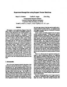
where g(x) is the decision function of a classifier, and R(I) represents the pattern space. The thresholding criterion states that we are taking the value of the discriminant function as a representation of the proximity to the in-class samples (Figure 1). This implies that the discriminant function should be able to create a “local” decision region, instead of a “global” one. Otherwise a confuser far away from the class center can easily be accepted as an object of interest. Hence in verification systems the actual topology of the classifier is rather important for rejection of confusers. Figure 1 For the problem of SAR/ATR, the classifier should be able to classify the targets in the training set as well as their variants (different serial numbers), and to reject confusers, all at a reasonable level. In this paper, SVMs are utilized to perform the task of target recognition and confuser rejection. As a comparison, perceptrons trained with the minimum squared error (MSE) criterion (the delta rule) [17] and structural risk minimization (SRM) are also used to perform the same tasks. The theoretical background of MSE and SRM are given in Section II. Experimental results and discussion are given in Section III and IV, respectively.

II. Learning Criteria for Empirical and Structural Risk Minimization Let us consider a two-class classification problem, where the training set is described as X := {x1 , , ..., x m }, xi ∈ R n , and labels as Y := { y1 , , ..., ym } ⊆ {−1,1} .

6

2.1 Perceptron Criterion and the Minimum Squared Error Criterion A simple classifier that can solve a linearly separable task is the perceptron [29], and its linear decision function is represented as g ( x) = sgn (w ⋅ x + b)

(5)

where (w ⋅ x) indicates the inner product, and sgn(.) is a signum function. The perceptron criterion (or the risk functional) is defined as [29] J ( w) =

å w⋅x

xi∈E x

i

+b

(6)

where the summation is over the set of Ex of patterns that are mis-classified by the perceptron, and ⋅ represents the absolute value. For linearly separable problems, the algorithm converges in a finite number of iterations. Unlike the perceptron criterion (6) which considers only the mis-classified patterns, the MSE criterion takes into account the entire training set, which is defined as the squared error ( L2 norm) between the desired output and actual output, m

J ( w) = å ( y i − g ( w, x i )) 2

(7)

i =1

To get a continuous differential output, a sigmoid function is used instead of the signum,

g ( w, x) =

1 1 + exp(− w ⋅ x + b)

(8)

The delta rule, which is a gradient based algorithm can be used to train the network [17]. Since the samples that produce larger errors are closer to the boundary, the MSE risk functional (7) will place the decision surface at a location that predicts better and more consistently the correct class assignment than the perceptron criterion does.

7

Taking into consideration of the model complexity, one can use regularization theory as indicated in Equation (1). Here a cost functional with a weight decay [37] term is utilized in the experiments,

J ( w ) = å ( y i − g ( w , x i )) 2 + λ ⋅ w

2

(9)

i

The parameter λ has to be experimentally determined.

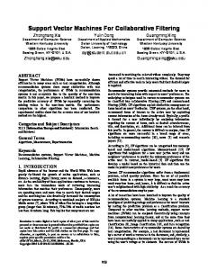
2.2 Criteria for Structural Risk Minimization The delta rule with weight decay implements criterion (1). In this section, an alternative learning criterion called structural risk minimization (SRM) is considered. Two applications of this learning methodology are briefly reviewed, i.e., Optimal Hyperplane (OH) and SVM. The interested reader is referred to [35] for a full treatment. (1). The Optimal Hyperplane The training set of Section II is said to be separated by an Optimal Hyperplane if the following two conditions are satisfied. First, all the samples are separated without error (keep the empirical risk zero), and second, as illustrated in Figure 2, the distances between the closest vectors to the hyperplane are maximal. The separating hyperplane is described in the canonical form,

yi ( w ⋅ x i + b) ≥ 1, i = 1, ..., m

(10)

Figure 2 It is easy to prove that the margin between the two hyperplanes H1 : w ⋅ xi + b = 1 and

H 2 : w ⋅ x i + b = −1 is d = 2 / w . Thus, to find a hyperplane that satisfies the second 2

condition, one has to solve the quadratic programming problem of minimizing w ,

8

subject to constraint (10). The solution to this optimization problem is given by the saddle point of a primal Lagrange functional, LP =

1 w 2

m

− å α i [ y i ( w ⋅ x i + b) − 1]

2

(11)

i =1

where α i , i = 1, ..., m , are positive Lagrange multipliers. Since (11) is a convex quadratic programming problem, it is equivalent to solve the “dual” problem [9]: maximize LP , subject to the constraints that the gradient of LP with respect to w and b vanish, which gives the simpler conditions, w = å α i yi x i

(12)

åα y

(13)

i

i

i

=0

i

Substituting (12) and (13) into (11), we get the dual formulation by the following vector representation, 1 LD = ΛT 1 − ΛT CΛ 2 T s.t. Λ Y = 0 Λ≥0

(14)

where ΛT = (α1 , ...,α m ) , Y T = ( y1 , ..., y m ) , 1T = (1, ... , 1) is an m-dimensional all-ones vector, and C is a symmetric m by m correlation matrix with elements C ij = y i y j x i ⋅ x j , i, j = 1, ..., m . Notice that there is a Lagrange multiplier α i for every

training sample. In the solution, those points with α i > 0 are called “support vectors” (SV), and lie on either H 1 or H 2 . The decision surface is made by

g ( x) = sgn( å yiα i x i ⋅ x + b) i∈SV

9

(15)

(2). The Soft Margin Hyperplane More generally, when dealing with non-linearly separable patterns, we will introduce positive slack variables ξ i , i = 1, ...., m , in the constraint (10), i.e., y i (w ⋅ x i + b) ≥ 1 − ξ i

(16)

For an error to occur, the corresponding ξ i must exceed unity, thus

åξ i

i

is an upper

bound on the number of training errors. In this case, the risk functional to minimize is,

L = w / 2 + λ (åi ξiσ ) k 2

(17)

subject to constraint (16), where λ is a parameter to assign a penalty to training errors. For any positive integer k, this is a convex programming problem. For sufficiently large

λ and sufficiently small σ, the parameters w and bias b determine the hyperplane that minimizes the number of errors on the training set and separate the rest of the elements with maximal margin. Note that the problem of constructing a hyperplane which minimizes the error on the training set is general NP-complete. To avoid this difficulty the case of σ = 1 is considered in this paper, where the solution is called the soft margin hyperplane. If we take k = 2 in (17), the optimization remains a quadratic programming problem of maximizing as LD = Λ T 1 −

1é T δ2ù + Λ CΛ 2 êë λ úû

(18)

s.t. Λ T Y = 0 δ ≥0 0 ≤ Λ ≤ δ1 where δ is a scalar, and the constraint implies that the smallest admissible value is

δ = α max = max(α 1 , ..., α m ) [6]. Therefore, to construct a soft margin hyperplane, one

10

can either solve convex programming problem in the m dimensional space of the parameter vector Λ , or solve the quadratic programming problem in the dual m+1 space of Λ and δ [6]. (3). Support Vector Machine Until now, all the previous architectures create the decision functions in the input space that are linear functions of data. Then one may ask how can the above method be generalized to the case of a nonlinear decision functions in a feature space? One alternative is to map the data to some other high dimensional Euclidean space (feature space) using a nonlinear mapping φ : R d → E . There is evidence provided by Cover’s theorem [22] that a complex pattern classification problem cast in a higher dimensional space is more likely to be linearly separable than in a lower dimensional space. The advantage of this method is that it de-couples the numbers of free parameters of the learning machines from the input space dimensionality [22]. In this way, the decision rule of (15) is implemented in the new feature space, i.e., g ( x) = sgn( å y iα iφ ( xi ) ⋅ φ ( x) + b) i∈SV

Using kernel functions K(x,y) that obey the Mercer condition [6, 28], the discriminant can be written g ( x) = sgn( å y iα i K ( x i , x ) + b)

(19)

i∈SV

The advantage of using kernel function is that instead of calculating the inner product of

φ ( xi ) ⋅ φ ( x) in the feature space, we can do it in the input space by using K ( xi , x) . This learning machine is the so-called Support Vector Machine. Correspondingly, the task of training a SVM is to maximize

11

1é δ2ù LD = ΛT 1 − êΛT KΛ + ú λû 2ë s.t. ΛT Y = 0 δ ≥0 0 ≤ Λ ≤ δ1

(20)

where K is a symmetric m by m kernel matrix with elements k ij = yi y j K(x i ⋅ x j ). To describe the classification ability of either the OH or the SVM, the margin of an example ( x j , y j ) is defined as [31]

ρ f (x j , y j ) = y j g (x j )

(21)

where g ( x j ) is the decision function defined by (19). It will be observed in the following experiments that SVM tends to increase the margins associated with training examples and converge to a distribution in which most examples have large margins. Instead of quadratic programming an iterative algorithm called the Adatron [2] is used in our experiments to train the OH. This algorithm was recently extended to the kernel Adatron [11] and [12], so it can also train the SVM. The advantage of the Adatron algorithm is its conceptual and implementation simplicity. It precomputes the inner products (or the kernel computation) so it is memory intensive and can not be applied to large data sets. As an iterative algorithm we have to choose experimentally the step size, but the conceptual simplicity and its straight forward implementation make it a good choice for our case. We present the algorithm in the appendix. One final point to make is that the large margin training is intrinsically a discriminant training method that is applied to two classes. Hence if the problem at hand has more than two classes we have to train several classifiers (either one class versus all the others, or pairwise classification). Since we only used three classes we utilized here the pairwise training (2 different classifiers were trained per class).

12

III. Experimental results In this paper, SAR ATR experiments were performed using the MSTAR database to classify three targets. The image data are composed of 80 by 80 SAR images chips roughly centered on three types of military vehicles: the T72, BTR70, and BMP2 (the T72 is a tank and the other two vehicles are armored personnel carriers). Examples of the SAR images are shown in Figure 3. These images are a subset of the 9/95 MSTAR (Moving and Stationary Target Acquisition and Recognition) Public Release Data, where the pose (aspect angles) of the vehicles lies between 0 to 360 degrees. Only target images are used here so there is no need for the focus of attention. This image set was chosen because there is available in the open literature a pilot study that can be used as a base for further comparisons [36]. Figure 3 We normalize the L2-norm of all the images from the training and testing sets, and utilized directly the images as inputs to the classifier. This pre-processing was kept at a minimum because the targets in the MSTAR database were in the same open field background, and the radar was carefully calibrated. If the operations of re-centering, intensity matching and background masking (as done in [36]) were performed better accuracy should be possible, but a longer effort would have been necessary to conduct the testing. The training set for the close set classification contained SAR images taken at a depression angle of 17 degrees, while the testing set depression angle is 15 degrees. Therefore the SAR images between the training and the testing sets for the same vehicle at the same pose are different. Variants (different serial number) of the three targets were

13

also used in the testing set for the open set experiments, as illustrated in Table 1. The size of the training and testing sets is 698 and 1365, respectively. Table 1: Training and Testing Set Training set

size

Testing set

size

T72 (Sn_132)

232

T72 (Sn_132)

196

T72 (Sn_812)

195

T72 (Sn_s7)

191

BTR70 (Sn_c71)

233

BTR70 (Sn_c71)

196

BMP2 (Sn_c21)

233

BMP2 (Sn_c21)

196

BMP2 (Sn_c9566)

196

BMP2 (Sn_c9563)

195

The SAR images are very noisy due to the image formation and lack resolution due to the radar wavelength, which makes the classification of SAR vehicles a non-trivial problem [23]. Unlike optical images, the SAR images of the same target taken at different aspect angles show great differences, which precludes the existence of a rotation invariant transform. This results from the fact that a SAR image reflects the fine target structure (point scatter distribution on the target surface) at a certain pose. Parts of the target structure will be occluded when illuminated by the radar from another pose, which results in dramatic differences from image to image taken with angular increments of only a few degrees. In order to cope with these problems, template matching uses closely spaced poses (~ 10 degrees) to form the template [36]. Template matchers are OCON classifiers, which are not trained discriminantly [20]. We are experimenting with a different classifier architecture, based on more powerful classifiers trained discriminantly (ACON) and a pose estimator (see Figure 4). The input space is divided using the pose information [25]

14

and twelve sub-classifiers were trained one for each 30 degrees sector of aspect angle with data from all the three classes. We have created a pose estimator based on mutual information that is able to determine the pose of all MSTAR targets with an error less than 8 degrees [39]. In these results we assume that the pose estimator is error free The large sector size was chosen to differentiate our approach from the closely spaced poses, but the sector has not been optimized for best performance. Figure 4 We compared three classifiers: (1) A perceptron trained with the delta rule and weight decay, with a single layer structure of 6,400 input units and 3 output units. (2) An OH (the same perceptron as in (1) but trained for large margin). (3) A Support Vector Machine based on the Gaussian kernel, with the kernel size chosen as the average Euclidean distance between training patterns. Both the OH and the SVM were trained with the Adatron algorithm with bias and soft margin algorithm [11,12] (See Appendix).

4.1 Classification Results A close set classification experiment was performed first. The perceptron was trained with a learning rate of 0.5 and a weigth decay of 10E-5. It is known that a perceptron is still very much related to the template matcher, but where each training image is nonlinearly weighted to create a discriminant template for the class. Figure 5(a) depicts images of the input weight matrices (white means high value) for each of the three output nodes for one of the sector classifiers (0-30 degrees aspect angle). Compared with the input SAR images in Figure 3, one can see that the weight images emphasize some of the point scatters of the targets, and suppress the background. Thus, effectively the perceptron is working with the discriminant and persistent scatters of each class for the

15

given sector. This has been the goal of model based ATR [21], but here the result is obtained through training and in a much simpler way. The OH uses the same architecture as the perceptron, but the training principle is different. Instead of training the weight vector itself using MSE, one trains the Lagrange multipliers using the SRM principle. Here we employed the Adatron algorithm [11,12] in a pair-wise training among the three classes (i.e., T-72 vs. BMP2, BMP2 vs. BTR70, and BTR70 vs. T72). In our experiments the advantage is obvious, since the number of training examples is much smaller than the dimensionality of the input space, so there are fewer parameters to be trained. Figure 5(b) shows the weight distributions for the OH obtained from the Lagrange multipliers using (12). Comparing with Figure 5(a), one can see many differences that result from the ERM an SRM training criteria. While the perceptron emphasizes the discriminant point scatters for each class, the OH works more with the pairwise differences and does not seem to concentrate as much on the point scatters. Figure 5

We used the Adatron and kernel Adatron algorithms with a stepsize of 0.01 to train the OH and SVM, which use the same training principle, but have different architectures. Figure 6 illustrates the learning curves and margin distribution for the OH classifier and SVM, where the margin distribution graph is defined as the sum of the margins (Equation (21)) of the training set as a function of number of iterations [31]. We also monitored the error in the test set (dashed line) for analysis purposes. In Figure 6(a), the learning curve for the OH reveals that the training error dropped to zero in 70 iterations, but the testing error continued to drop from 22 to 8 in the next 450 iterations. In Figure 6(b) the error for the SVM only took about 20 iterations to reach zero while the testing error continued to 16

drop from 22 to 6 in the following 200 iterations. Meanwhile, the sum of margins of the training set continued to increase quickly even after the training error is zero. This means that there is fine-tuning of the decision boundary even after the training set error reaches zero. This is impossible with the delta rule, and shows the intrinsic difference between SRM and ERM training. The test error plots also shows another difference with respect to the MSE training. There is no over-training with the SRM principle since the error monotonically decreases as the margins are maximized. Hence, the stop criterion for training should be based not on the error but by monitoring the margin. Comparing the learning curves and margin distribution graphs in Figure 6 (a) and (b), we find that the SVM converges faster than the OH, but the margins are identical for our data. This indicates similar performance.

Figure 6

Table 1 shows the classification results (misclassification rates) of the three classification methods. The misclassification rates Pe of the large margin classifiers were around 9% while the perceptron achieved 12% approximately. It reveals that the OH and the SVM had a better classification performance than the perceptron. We also conclude that there is no advantage in classification accuracy of the SVM over the OH. This may be related to the high dimensionality of our data set. The networks were run several times with different initial conditions and learning rates and the results of Table I were repeatable. Table 1 Misclassification rates (%) of the classifiers

17

BMP2

BTR70

T72

Average

Perceptron

9.88

0.51

17.87

11.94

OH

6.13

1.02

15.64

9.45

SVM

9.03

0.51

11.86

9.01

4.2. Verification Results A critical problem in ATR is how to discriminate between targets and confusers. To reject confusers, thresholds are set for all three classifiers, and performance in terms of missed detections and false alarms is measured in a ROC curve. In the verification experiment the previously trained classifiers were tested in an enlarged test set with two confusers, D7 and 2S1. The baseline for the comparison is the template matching method using basically the same MSTAR target mix [36], where a power normalized template matcher with a mask individualizing the targets was developed with templates at 10 degrees increments. This preprocessing is much more involved than the one used in our design and may bias the results in favor of the template matcher. For all the four classifiers, a threshold was individually set for each method to keep the probability of detection, Pd, equal to 0.9 in the testing set. Here Pd is defined as the ratio of number of targets detected and the total number of targets (A Pd of 0.9 is typically used in MSTAR). The recognition results are listed in Table 2. The misclassification rate, Pe , is defined as the ratio of number of targets incorrectly classified over the number of targets tested. The first row gives the result for the template matcher as reported in [36]. The average Pe of the perceptron, OH, and SVM were 6.67%, 5.42% and 5.13%, respectively. They are all better than the template matching, which is 9.60%.

18

Concomitantly with these experiments conducted in our laboratory, another group was applying SVMs to the MSTAR data [21]. In their paper, a SVM classifier was used to classify the same target mix in MSTAR, but using a polynomial instead of a Gaussian kernel function, and trained with the standard and more involved quadratic programming approach. The reported misclassification errors are around 6.6%-7.2%, slightly worse than our results. Table 2.

Misclassification rates and confuser rejection rates (%) BMP2

BTR70

T72

Average

Confuser rejection

Template

11.58

2.04

10.14

9.60

53.47

Perceptron

9.71

0.00

5.84

6.67

27.19

OH

8.69

0.51

3.78

5.42

38.50

SVM

4.94

0.00

7.04

5.13

68.80

When confusers were added to the test set, the SVM showed the highest rejection rate of 68.80%, while the optimal hyperplane presented a rejection rate of 38.50%, and the perceptron 27.19%, respectively. The template matching showed a rejection rate of 53.47% , which is better than the perceptron and OH, but still worse than the SVM. These rejection results may seem to contradict the classification results, but in fact they are easily interpreted if one groups the classifier’s discriminant function type in local or global. In fact, the best performers in rejection are the SVM (which uses the Gaussian kernel) and the matched filter, which is also a local discriminant. The global discriminant classifiers (OH and perceptron) were unable to reject confusers as effectively.

19

Table 3 Confusion matrices and misclassification rates (%) of the classifiers and the confuser rejection rates (%) when Pd =0.9 BMP2

BTR70

T72

Rejection

BMP2

483

59

9

36

BTR70

4

188

0

4

T72

43

16

427

96

2S1

111

83

38

42

D7

16

4

3

251

(a) Template matching BMP2

BTR70

T72

Rejection

BMP2

436

16

41

83

BTR70

0

194

0

2

T72

18

16

502

51

2S1

9

105

100

60

D7

29

68

88

89

(b) perceptron

BMP2

BTR70

T72

Rejection

BMP2

443

9

42

88

BTR70

0

193

1

2

T72

16

6

519

46

2S1

9

50

117

98

D7

53

9

99

113

(c) optimal hyperplane BMP2

BTR70

T72

Rejection

BMP2

511

14

15

47

BTR70

0

195

0

1

T72

31

10

453

88

2S1

57

24

10

183

D7

53

0

27

145

(d) support vector machine

20

We present in Table 3 the confusion matrices for each classifier at Pd = 0.9. In terms of rejection each system makes its own type of mistakes. For instance, the template matcher has difficulty with the 2S1 (confused with the BMP2), while the other 3 classifiers have a more equilibrated performance, and are progressively better at rejecting confusers. The SVM classifier improves the rejection of the template matcher from 53% to 68% (reduces misdetections from 255 to 171) while providing a better error rate, hence it is a better classifier for verification. Figure 7 We note that Table 2 only provides results for probability of detection Pd = 0.9, corresponding to only one point on the ROC curve. To give an overall performance comparison, the receiver operating characteristics (ROC) curves of the three classifiers are shown in Figure 7. It is observed that the SVM shows much better target recognition and confuser rejection performance than the two other classifiers. We have to point out that the ROC for the BTR70 is much better than the others because there are no variants for this vehicle in the test set.

VI. Discussion and Conclusion Our tests in SAR/ATR and the choice of our classifiers enable us to conclude some very interesting points about topology of classifiers and training criterion. This is illustrated briefly in Table 4. Table 4. Topology of classifier vs. training criterion

ERM

SRM

Global discriminant

Perceptron

Optimal Hyperplane

Local discriminant

Radial Basis Function

Support Vector Machine

21

Notice that we have the same classifier topology trained with different principles: global discriminant perceptron is trained with either the ERM (e.g., delta rule with weight decay) or with SRM (or large margin rule). We also have the same basic training principle (SRM or large margin) applied to two different topologies, the OH perceptron with global discriminant and the SVM with Gaussian kernel (the local discriminant). Finally, we have two different classification problems: the close and open sets. Hence we can confidently draw the following conclusions: For close set classification problems the generalization of the large margin classifiers outperforms the ERM principle in the MSTAR data set. We say this because the OH outperforms the perceptron trained with the delta rule. The performance improvement is substantial but not dramatic. We thought that the SRM had the potential to produce even better classifiers, but obviously, this depends on the structure of the data clusters. By analyzing the learning criteria, we can see that the modified ERM learning criterion (9) has a L2 norm in both the training set error and the regularization. Although never designed for large margin, the MSE positions the decision surface at a location with a “safe margin” between the vehicle classes. This was unexpected in particular because the size of the training data is much smaller than the input data dimensionality, which raises many concerns about generalization. Different from (9), the SRM criterion (11) maximizes the margin by using a L1 norm in the training set error, and a L2 norm in the regularization. The major difference between these schemes is the training set error norm. We analyzed what this difference in norm effectively means in terms of the number of degrees of freedom of the classifier. The perceptron trained with the delta rule and weight

22

decay has 6,400 weights per class where the weight distribution is shown in Figure 5. In the OH classifier the Lagrange multipliers play a similar role to the weights in the perceptron. Figure 8 shows the Lagrange multipliers αi for the OH and SVM. We first note that the number of αi is related to the number of training samples, instead of the dimensionality of inputs to the classifier. This is the big difference between the two methods: large margin training decouples in a very effective way the input space dimension from the number of features used, while the MSE is stuck with the input data dimensionality. Only changing the topology (increasing the number of layers) can help a classifier trained with MSE decouple the feature space from the input space, but then the designer is faced with the problem of choosing the number of hidden PEs without a good theory to guide in the design. Moreover, the large margin training can still assign “importance” to each input data sample by the value of the Lagrange multipliers: when αi are far from zero they are called support vectors, because they are the ones that define the position of the decision surface. In Figure 8 the values of the multipliers are shown for both the OH and SVM of the first sector among the 12. It is seen that most of the αi are greater than zero, which means that for our ATR application almost all the samples are kinds of support vectors. This is due to the small data set and the high dimensionality of the input space, and each sample in the data set has to play a role in forming the decision boundary. This small ratio of data samples to space dimensionality may also explain why the SVM did not outperform the OH in our close-set classification results. Figure 8 When the classification is open set, the classifier topology plays a more important role than the training principle. This means that open and close set classification are

23

really two different problems, where generalization is not the only difficulty. In open set classification the learning machine is presented with samples that are beyond the training set classes, i.e. that appear in very different areas of the pattern space. We (and others) use the idea of thresholding the output of the classifiers to decide about the degree of partnership to the in-class samples. Note that this implies that the class posterior distribution must be a good representation for the probability density function. With this thresholding methodology the design for large margin was not the major factor in performance. What is important here is to choose topologies that enforce local class discriminants. The SVM maps a confuser far away from the “local” decision region onto a location close to the origin of the feature space, which promises a reliable rejection. Perceptrons are notorious for their global discriminants (hyperplanes) so they perform poorly in these tasks (irrespective of the learning principle) even when compared with template matchers that are known to generalize poorly (because they are linear systems [8]). When we choose topologies that enforce local discriminants a large margin classifier still seems more robust to confusers. Unfortunately, the comparison of the SVM with the template matcher is not very appropriate since the template matcher is unable to exploit covariance information, and they are really embedded in two different classifier designs (see below). A more appropriate test would have been the comparison of the SVM with a radial basis function network (RBF). This point had been addressed in reference [30], where the SVM and RBF had been compared using a real-world pattern recognition experiment (handwritten digits recognition), and the result showed that the SVM achieves higher recognition accuracy than the RBF.

24

The performance comparison between template matchers and the other three methods (SVMs, OH and perceptrons) is not straight-forward because the differences are not only in classifier structure but also in classifier design. In fact the template matcher constructs a template from all the poses of a single vehicle (OCON), while all the other classifiers are trained with all the vehicles in the training set (ACON), but only across 30 degree aspect angles. Our classifier design exploits a divide-and-conquer approach in the sense that we realize that one of the difficulties in SAR/ATR is the huge dependence of the signatures with aspect angle. Hence, we reason that it should be much simpler to discriminate targets if we compare vehicles aligned for pose. In order to implement this principle we first estimate the pose and then derive classifiers for a subset of the pose angles within a sector (30 degrees in these experiments). The results presented in this paper show that in fact the SVM outperforms the template matcher in both accuracy and in confuser rejection (the OH and perceptron also outperform the template matcher in accuracy). But there are so many differences between SVMs and template matchers that we can not say univocally that this difference is due to our classifier design. There are a number of design parameters that were not fully considered in our approach. Probably the most important is the sector size. We saw that the discriminability of targets varied widely over aspect, but we kept the same sector size in the design. Sectors that produce poor results should be broken down in smaller sectors to improve discriminability. But of course there is a lower limit on the sector size due to pose estimator accuracy and also on the available data to train the classifiers. This tradeoff should be further investigated. Acknowledgments: This work was supported by a DARPA grant F33615-97-1-1019.

25

Appendix: Algorithm of Kernel Adatron with Bias [12] 0. Define m

f AD ( x i ) = y i ( å y j α j k ( x i , x j ) + b) j =1

M AD =

min f AD ( xi )

i∈{1,...,m}

1. Initialization setup: Lagrange multipliers α i , i ∈{1, ..., m} , learning rate η , bias b, and a small threshold t. 2. While M AD ≥ t 3.

Choose pattern x i , i ∈{1, ..., m}

4.

Calculate a update δ i = η (1 − f AD ( x i ))

5.

If (α i + δ i ) > 0, α i = α i + δ i , b = b + y i δ i

6. End While

References 1. H. Akaike. A new look at the statistical model identification IEEE Transactions on Automatic Control, 19:716-723, 1974.

2. J. Anlauf and M. Biehl. The Adatron: an adaptive perceptron algorithm. Europhysics Letters, 10(7): 687-692, 1989.

3. L. Breiman. Bagging predictors. Technical report No.421, University of California, Berkeley, 1994. 4. R. Chellappa, C. Wilson, and S. Sirohey. Human and Machine Recognition of Faces: A Survey. Proceedings of the IEEE, 83(5), 1995. 5. C. Burges. “A tutorial on support vector machines for pattern recognition”. Data Mining and Knowledge Discovery, 1998.

6. C. Cortes and V. Vapnik. “Support vector networks”. Machine Learning, 20: 273297, 1995 7. R. Courant and D. Hilbert. Methods of mathematical physics, Interscience, 1953. 8. J. Fisher and J.C. Principe. “Recent advances to nonlinear MACE filters”. Optical Engineering, 36(10): 2697-2709, 1998.

26

9. R. Fletcher. Practical methods of optimization. Great Britain: John Wiley and Sons, Inc., 2nd edition, 1987. 10. Y. Freund and R. Schapire. “A decision-theoretic generalization of on-line learning and an application to boosting”. In Proceedings of the 2nd European Conference on Computational Learning Theory, 1995.

11. T. Frieβ, N. Cristianini and C. Campbell. “The kernel-Adatron algorithm: a fast and simple learning procedure for support vector machines”. In Machine Learning: Proceedinds of the 15th International Conference, Shavlik, J. ed., Morgan Kaufmann

Publishers, San Francisco, CA, 1998. 12. T. Frieβ. “Support vector neural networks: the kernel Adatron with bias and softmargin”. Research report, University of Sheffield, UK, 1998. 13. K. Fukunaga. Statistical pattern recognition. 2nd ed. San Diego, CA:Academic Press. 14. H. Gish and M. Schimdt. “Text-independent speaker identificatio”. IEEE Signal Processing Magazine, 11: 18-32, 1994.

15. F. Girosi. “An equivalence between sparse approximation and support vector machines”. Neural Computation, 10(6): 1455-1480, 1998. 16. M. Gori and F. Scarselli. “Are multilayer perceptrons adequate for pattern recognition and verification?” IEEE Transactions on Pattern Analysis and Machine Intelligence, 20(11): 1121-1132, 1998. 17. S. Haykin. Neural networks: A comprehensive foundation, Englewood, NJ: Macmillan College Company, Inc, 1994. 18. C. W. Helstrom, Statistical theory of signal detection. 2nd edition, Pergamon Press Inc., 1968. 19. B. Juang and S. Katagiri. “Discriminative learning for minimum error classification.” IEEE Transactions on Signal Processing, 40(12): 3043-3054, 1992.

20. S. H. Lin, S. Y. Kung, and L.J. Lin. “Face recognition/detection by probabilistic decision-based neural network”. IEEE Transactions on Neural Networks, 8(1): 114132, 1997. 21. M. Bryant and F. Garber (1999) “SVM classifier applied to the MSTAR public data set”, Algorithms for Synthetic Aperture Radar Imagery VI, E. Zelnio, Eds., Proceedings of the SPIE, 3721, 355-360.

27

22. N. Nilsson, Learning Machines: foundations of trainable pattern-classifying systems, McGraw-Hill, Inc., 1965. 23. L. Novak, G. Owirka, W. Brower and A. Weaver. “The automatic target recognition system in SAIP”, The Lincoln Lab Journal, 10(2), 187-202, 1997. 24. J. Principe, A. Radisavljevic, J. Fisher, and L. Novak. “Target prescreening based on a quadratic Gamma discriminator”. IEEE Transactions on Aerospace and Electronic Systems, 34(3): 706-715, 1998a.

25. J. Principe, Q. Zhao and D. Xu. “A novel ATR classifier exploiting pose information”. In Proceedings of Image Understanding Workshop, pp.833-836, Monterey, CA., Nov. 1998b. 26. M. Priestley, Spectral analysis and time series, New York: Academic Press, 1981. 27. J. Rissanen. “Modeling by shortest data description”. Automatica, 14: 465-471, 1978. 28. J. Rissanen, Stochastic complexity in statistical inquiry, Singapore: World Scientific, 1989. 29. F. Rosenblatt. The Perceptron: “A probabilistic model for information storage and organization in the brain”. Psychological Review, 65: 386-408, 1958. 30. B. Schoolkopf, K. Sung, C. Burges, F. Girosi, P. Niyogi, T. Poggio, and V. Vapnik. “Comparing support vector machines with Gaussian kernels to radial basis function classifiers”. IEEE Transactions on Signal Processing, 45(11): 2758-2765, 1997. 31. R. Schapire, Y. Freund, P. Bartlett, and W. Lee. “Boosting the margin: A new explanation for the effectiveness of voting methods” Annals of Statistics, 1998. 32. M. Schimdt. “Identifying speaker with support vector networks”. In Interface’96 Proceedings, Sydney, 1996.

33. A. Tikhonov and V. Arsenin. Solutions of ill-posed problems. Washington, D.C.: W.H. Winston, 1977. 34. V. Vapnik. Statistical learning theory. John Wiley and Sons, Inc., New York, 1998. 35. V. Vapnik. The nature of statistical learning theory. New York: Springer-Verlag, Inc., 1995. 36. V. Velten, T. Ross, J. Mossing, S. Worrell, and M. Bryant. “Standard SAR ATR Evaluation Experiments using the MSTAR Public Release Data Set”. Research Report, Wright State University, 1998.

28

37. A.S. Weigend. “Generalization by weight elimination with application to forecasting”. In Advances in Neural Information processing Systems, 3:875-882, 1991. 38. Q. Zhao and Z. Bao. “Radar target recognition using a radial basis function neural network”. Neural Networks, 9(4), pp.709-720, 1996. 39. Q. Zhao, D.X. Xu, and J. Principe (1998). “Pose estimation of SAR automatic target recognition.” In Proceedings of Image Understanding Workshop, Monterey, CA., Nov. 1998, pp.827-832. 40.

Q. Zhao, and J. Principe (1999). “From hyperplanes to large margin classifiers: Applications to SAR ATR”. Automatic Target Recognition IX, F. Sadjadi Ed. Proceedings of the SPIE, 3718, 101-109.

41.

Zhao, Q., Principe, J.,Brennan, V., Xu, D.,and Wang,Z. (2000). "SAR Automatic Target Recognition with Three Strategies of Learning and Representation". Optical Engineering, May.2000 (to be published)

29

Figure 1. An illustration of a two-class classification problem. In the left figure, a “global” discriminant function divides the whole sample space into two parts. In the right figure, two “local” decision regions are formed to keep the confusers away from the class region of interest. Figure 2. A two-class linearly separable problem (balls vs. triangles). The optimal hyperplane (solid line) intersects itself halfway between the two classes, and keeps the margin maximal. The samples across the boundary H1 or H2 are support vectors. Figure 3. (a) Illustration of pose; (b) SAR images of target T72, BTR70 and BMP2 taken at different aspect angles Figure 4 The classifier topology is depicted. First a pose estimator is applied to the image and determines the approximate pose of the target, then a classifier is chosen according to the result of pose estimation. Figure 5 (a) Weight distribution of the perceptron trained with Equation (9). The weights connected input nodes with three output nodes, respectively, of the classifier covering aspect angles from zero to thirty degrees. Compared with the images in Figure 3, they resemble the targets’ features. (b) Weight distribution of OH, obtained with the Lagrange multipliers (T72-BTR70, BTR70-BMP2, BMP2-T72). Figure 6. Learning curves and margin distribution graphs for the Optimal Hyperplane (OH) and SVM, where the margin distribution graph is defined as the sum of the margins of the training set as a function of number of iterations. The learning curves are shown above the corresponding margin distribution graphs. Each learning curve and margin distribution graph shows the training error/margin (with solid line) and testing error/margin (with dash-dot line), respectively. It is revealed that after the training error dropped to zero, the testing error still continued dropping, and the sum of margins continued increasing.

30

Figure 7. ROC curve of the three classifiers, using the test sets against the two confusers. Figure 8 shows the values of the Lagrange multipliers of the trained (a) OH and (b) SVM, where most of them are greater than zero and thus support vectors by definition.

31

Figure 1

Margin

H2

H1

Figure 2

32

(a)

(b)

Figure 3

33

0 Feature + Classifier Pose Estimator

360 Deg selector

Figure 4

34

vehicle vehicle vehicle. vehicle

(a) perceptron

(b) OH

Figure 5

35

(a) OH

(b) svm Figure 6

36

(a) Perceptron

(b) OH

Figure 7

37

(c) SVM

Figure 7

38

(a) OH

(b) svm Figure 8

39

40