On-line Handwriting Recognition with Support Vector Machines--- A ...

publ. in Proc. of the 8th Int. Workshop on Frontiers in Handwriting Recognition (IWFHR), pp. 49–54, 2002. ftp://ftp.informatik.uni-freiburg.de/papers/lmb/ba_ha_bu_iwfhr02.pdf

On-line Handwriting Recognition with Support Vector Machines— A Kernel Approach Claus Bahlmann, Bernard Haasdonk and Hans Burkhardt Computer Science Department Albert-Ludwigs-University Freiburg 79110 Freiburg, Germany {bahlmann,haasdonk,burkhardt}@informatik.uni-freiburg.de

Abstract

tions. Some further properties are commonly seen as reasons for the success of SVMs in real-world problems: the optimality of the training result is guaranteed, fast training algorithms exist and little a-priori knowledge is required, i.e. only a labeled training set.

In this contribution we describe a novel classification approach for on-line handwriting recognition. The technique combines dynamic time warping (DTW) and support vector machines (SVMs) by establishing a new SVM kernel. We call this kernel Gaussian DTW (GDTW) kernel. This kernel approach has a main advantage over common HMM techniques. It does not assume a model for the generative class conditional densities. Instead, it directly addresses the problem of discrimination by creating class boundaries and thus is less sensitive to modeling assumptions. By incorporating DTW in the kernel function, general classification problems with variable-sized sequential data can be handled. In this respect the proposed method can be straightforwardly applied to all classification problems, where DTW gives a reasonable distance measure, e.g. speech recognition or genome processing. We show experiments with this kernel approach on the UNIPEN handwriting data, achieving results comparable to an HMMbased technique.

For the solution of on-line handwriting recognition (HWR) tasks researchers presently use classification methods which are based on a Bayesian generative approach: hidden Markov models (HMMs) model a sequence of class conditional densities based on (and thus restricted to) a certain function class. A discriminant function is obtained in a second step using Bayes’ rule. Indeed HMMs have proven to deal very well with the complex on-line handwriting data structure. This is usually a variable-size sequence of feature vectors that may have been distorted in particular ways, each vector computed from sampled coordinates of the pen tip curve. While the generative approach is indeed optimal if the underlying models are accurate, it can perform poorly if this assumption is not fulfilled. In most practical applications, also in HWR, the latter is often the case. In these situations discriminative approaches which do not aim to estimate class conditional densities but directly address the discrimination by creating class boundaries are a promising choice. As noted above, SVMs belong to this category of classifiers.

1. Introduction The utilization of support vector machine (SVM) [2, 4] classifiers has gained immense popularity in the last years. SVMs have achieved excellent recognition results in various pattern recognition applications [4]. Also in off-line optical character recognition (OCR) they have been shown to be comparable or even superior to the standard techniques like Bayesian classifiers or multilayer perceptrons [5]. SVMs are discriminative classifiers based on Vapnik’s structural risk minimization principle. They can implement flexible decision boundaries in high dimensional feature spaces. The implicit regularization of the classifier’s complexity avoids overfitting and mostly this leads to good generaliza-

However, so far no on-line HWR system using SVMs is known to the authors. In this respect this contribution is the first one incorporating SVMs into on-line HWR. The reason why SVMs have not been used in the past can be seen in the data structure mentioned above: common SVM techniques were developed for a feature space with a fixed dimension, whereas the on-line handwriting sequences vary in length and are temporally distorted. An ad-hoc solution to overcome this incompatibility—like a linear scaling of the writing to a fixed number of samples—is not promising to outperform standard HMM techniques, since it can49

It is convenient to model φ as a sequence of local transitions. We use the ones which are known as SakoeChiba transitions in the literature [15]. These only allow forward steps of size 1 in T , R or in both of them, i.e. φ (n + 1) − φ (n) equals (1, 0), (0, 1) or (1, 1). Usual dynamic programming and beam search strategies [11] are applied to reduce the computational complexity when minimizing (2). The DTW technique itself in combination with a minimum distance classifier [17, 18] as well as the incorporation of statistical knowledge to this concept [1] have been successfully applied to handwriting recognition.

not deal with the nonlinear, temporal variations in the data. In our view a successful approach should both embed the discriminative power of SVMs as well as the flexibility in coping with temporal distortions. A starting point for linking SVMs with sequential data is the so-called kernel, as will be shown. Some work has been done in other research areas dealing with kernels for sequential data. Jaakkola et al. [10] developed an SVM kernel in their application of protein homology detection and refer to it as Fisher kernel. Watkins [19] describes several explicit kernels for sequential data and shows that the joint probability of two sequences according to a pair HMM is a proper SVM kernel under certain conditions. Since the kernels mentioned above are still based on an estimation of generative parameters, we propose an alternative approach which is less complex and presumes less model knowledge: the Gaussian dynamic time warping kernel (GDTW). We shall start with a short review of dynamic time warping (DTW) and SVMs in the following section. Section 3 then introduces the GDTW kernel. Experimental results with this GDTW kernel on the UNIPEN [7] data and a comparison to UNIPEN results of other recognition techniques are presented in section 4. Section 5 provides a conclusion of this contribution.

2.2. Support vector classification Here, we provide a brief introduction to support vector classification. For more details and geometrical interpretations please refer to the standard literature, e.g. by Burges [2] or Cristianini and Shawe-Taylor [4]. Consider a two-class classification problem and a set of training vectors {Pi }i=1,...,M with corresponding binary labels Si = 1 for the “positive” and Si = −1 for the “negative” class. In classification an SVM assigns a label Sˆ to a test vector T by evaluating
αi Si K (T, Pi ) + b and Sˆ = sign (f (T )) . f (T ) =

2. Background

i

(3) The weights αi and the bias b are SVM parameters and adopted during training by maximizing

2.1. Dynamic time warping In DTW [15] a distance D (T , R) from two vector sequences T = (t1 , . . . , tNT ) and R = (r1 , . . . , rNR ) is determined. In on-line HWR the vectors ti ∈ IRF and rj ∈ IRF are usually computed from the local neighborhood of the i-th respectivej-th sampled point of the pen tip curve. See section 4.2 for the authors’ choice of ti and rj . Given a so-called alignment (or warping) path φ = (φ (1) , . . . , φ (N )) with φ (n) = (φT (n) , φR (n)) ∈ {1, . . . , NT } × {1, . . . , NR }(φ is introduced to align corresponding regions in the sequences T and R; see the textbook of Rabiner and Juang [15, Chapter4.7] for further details) and a local distance measure d, e.g. d (ti , rj ) = 2
ti − rj
, we define the alignment distance Dφ as the mean distance along a particular alignment path φ Dφ (T , R)

=

N  1
 d tφT (n) , rφR (n) . N n=1

LD =

φ

αi −

i

1
αi αj Si Sj K (Pi , Pj ) 2 i,j

(4)

under the constraints 0 ≤ αi ≤ C

and




αi Si = 0

(5)

i

with C a positive constant weighting the influence of training errors. K (·, ·) is the kernel of the SVM. A solution for the αi implies a value for b. The SVM framework gives some flexibility in designing an appropriate kernel for the underlying application. Many implementations of kernels have been proposed so far, one popular example is the Gaussian kernel   2 (6) K (Pi , Pj ) = exp −γ
Pi − Pj
.

(1)

If K (·, ·) is positive definite, (4)–(5) is a convex quadratic optimization problem, for which the convergence towards the global optimum can be guaranteed. However, obtaining this solution for real-world problems can be quite demanding and requires sophisticated optimization algorithms like

The DTW distance (or Viterbi distance) D (T , R) is defined as the alignment distance (1) along the Viterbi path φ∗ D (T , R) = Dφ∗ (T , R) = min {Dφ (T , R)} .




(2) 50

T

chunking, decomposition or sequential minimal optimization [4]. Usually αi = 0 for the majority of i and thus the summation in (3) is limited to a subset of the Pi , which therefore is called the set of support vectors. Extensions of the binary classification to the multi-class situation are suggested in several approaches [2, 13].

P2

P3

2

2

2

1

1

1

1

P4

P5 2

1

1

0

0

0

−1 0

1

2

φ∗

−1

1

2

−1

−1

−1

−1 −2

0

2

−2

0

2

−2

−1

0

1

2

−2

40

40

40

40

40

30

30

30

30

30

20

20

20

20

10

10

10

10

10

D (T , Pj ) K (T , Pj )

0

0

0

0

−1 −1

3. Gaussian dynamic time warping kernel

20

30

40

0 1

10

20

30

0.20 0.70

10

20

0.71 0.28

30

0

2

20 10

10

20

30

40

0.99 0.17

20

40

60

10.04 0.00

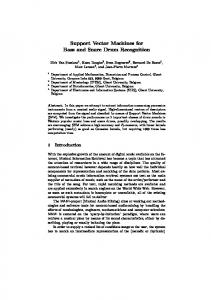
Figure 1. The Gaussian dynamic time warping (GDTW) kernel: Character patterns T (class “h”) and Pj , j = 1, . . . , 5 (classes “h”, “h”, “k”, “n”, “m”) are illustrated by the features x ˜ and y˜ (see section 4.2 for the definition). The values for the DTW distance D and the GDTW kernel evaluation K for γ = 1.8 are provided in the third and fourth row, respectively. The values show the obvious fact that similar patterns give small values for D and large for K. In the second row the Viterbi path φ∗ is illustrated: The sketched line traverses all aligned   point pairs φ∗T (n) , φ∗Pj (n) , n = 1, . . . , N in the NT × NPj matrix.

As indicated in the introduction, when dealing with sequential on-line handwriting data we cannot simply employ the basic SVM framework given by (3)–(6). Different feature vector sequences Pi , Pj and T cannot be embedded in the same vector space in general, as the necessary dimensions differ. However, an important property of (3)–(4) is that the vectors Pi , Pj and T appear only in form of kernel evaluations. Thus our objective, when adopting SVMs to sequential handwriting data, can be to state a kernel definition suitable to the particular properties of the sequential data. An obvious modification of (6) is to replace the squared 2 Euclidean distance
Pi − Pj
with the equivalent when dealing with temporally distorted, sequential signals—the DTW distance D (Pi , Pj ) described above. For two equally sized sequences and a linear alignment φ (n) = (n, n) even 2 the equation N · D (Pi , Pj ) =
Pi − Pj
holds. We therefore apply this modification and define the Gaussian DTW (GDTW) kernel for sequential data by K (Pi , Pj ) = exp (−γD (Pi , Pj )) .

P1

2

by randomly chosen characters Pi , Pj from the UNIPEN database turn out to violate the pd only weakly: For matrices of sizes up to 40 × 40 all λi were experimentally measured to be nonnegative. For larger matrices the sporadic missing pd was due to only a few negative eigenvalues with small absolute values compared to the other eigenvalues.

(7)

In the following we will abbreviate an SVM classifier with a GDTW kernel as SVM-GDTW. Figure 1 illustrates the GDTW kernel with some examples. A theoretical relevant property of (7) should be mentioned: as the DTW distance is not a metric (invalid triangle inequality in many cases), one could fear that the resulting kernel lacks some necessary properties, e.g. the positive definiteness (pd) noted in section 2.2. This would imply that the solution of the optimization algorithm is not guaranteed to be the global optimum. In fact general pd cannot be proven for (7), as simple counterexamples can be found. Nevertheless such kernels can produce good results like in our case and others [5, 8]. Recalling the fact that positive definite kernels are characterized by the property of generating kernel matrices Kij = K (Pi , Pj ) with solely nonnegative eigenvalues λi , some reasons for the good recognition rates may be the following: Firstly, the SMO algorithm is operating on 2×2 kernel matrices and such matrices provable always have nonnegative λi . The SMO algorithm therefore is expected to converge although no optimality can be guaranteed. Secondly, larger kernel matrices generated

4. Experiments 4.1. Data The experiments are based on the 1a, 1b and 1c section (digits, upper and lower case characters, respectively) of the UNIPEN [7] Train-R01/V07 database. For these sections the data set size is ≈ 16K, 28K and 61K, respectively. Examples of UNIPEN data were shown in figure 1. Training and test set were taken disjointly. It should be stated that UNIPEN consists of very difficult data due to the variety of writers and noisy or mislabeled data. We used the database without cleaning in order to be as comparable as possible to other classification reports.

4.2. Feature selection We model each vector ti of a sequence T = (t1 , . . . , tNT ) by three local features at the i-th samT xi , y˜i , θi ) . The quantipled point (xi , yi ): ti = (˜ 51

y −µ

x ties x ˜i = xiσ−µ and y˜i = iσy y are the pen coordiy nates normalized by the mean (µx , µy ) and y-deviation σy of all character’s sample points. The feature θi is the tangent  slope angle at√point i, approximated  by θi = ang (xi+1 − xi−1 ) + −1 · (yi+1 − yi−1 ) with √ −1 the imaginary unit and “ang” the complex angle function. Since θi is a circular measure, there is some special treatment necessary when computing the local distance 2 d (ti , rj ) =
ti − rj
. Instead of the usual difference ∆θ = (θ1 − θ2 ) we use the circular difference ∆mod θ = (θ1 − θ2 ) mod 2π with ∆mod θ ∈ (−π, π]. No pre-processing, such as re-sampling of the writing or reference line detection, is applied in this case. Each pattern is typically represented by about 10–80 sample points.

result, that for the dissimilar character pairs (a ↔ b, d ↔ m) classification errors are rare in both classification methods, actually are due to mislabelings. In a second category of two-class experiments the discrimination of character class pairs, which were shown to be similar and were frequently misclassified by SDTW, was examined. Table 1 illustrates, that for some of the selected character pairs (c ↔ e, b ↔ h) SVM-GDTW gives lower error rates than SDTW, for others (u ↔ v, y ↔ g) vice versa.

4.4. Multi-class experiments For a multi-class experiment we have chosen the DAGSVM approach [13]. DAG-SVM combines a set of twoclass SVMs into a multi-class classifier. For a K-class problem DAG-SVM contains K · (K − 1) /2 two-class classifiers, one for each class pair. During classification K − 1 two-class SVM evaluations are combined using a decision directed acyclic graph (DDAG) topology. For the multi-class case we used smaller UNIPEN subsets due to efficiency reasons (see section 4.5). We made experiments on two different dataset sizes in order to give an idea of the recognizer’s dependence on this quantity. Figure 2 gives a graphical illustration of an example classification showing a snapshot of our classification GUI. Table 2 summarizes classification error rates of a DAGSVM-GDTW classifier for the 1a/b/c UNIPEN sections and compares this result to other results on UNIPEN data collected from the literature. Though all experiments were computed on UNIPEN data, various reports used different character sets. Benchmarks were computed on miscellaneous versions and sizes of a UNIPEN database or some authors removed low quality/mislabeled characters, as indicated in the table’s last column. Thus in the following comparison we refer only to the experiments on a unique set. In the table we typed these values boldface. From the values it can be seen that DAG-GDTW-SVM achieves lower error rates than SDTW for the relative small training set. For the larger training sets DAG-GDTW-SVM and SDTW achieve comparable error rates. The higher performance of DAG-GDTW-SVM in comparison with SDTW on the small training set supports the statement that the statistical approach SDTW is highly dependent on accurate models, which cannot be satisfactorily gained from the relative small training set.

4.3. Two-class experiments We have trained the SVM-GDTW with the sequential minimal optimization (SMO) algorithm [14], using a third party Matlab SVM toolbox [3]. For the following experiments the SVM and kernel parameters were set to C = 1 and γ = 1.8, respectively. In the first investigation we were concerned whether an SVM-GDTW is able to classify clearly separable data. Hence we applied the SVM-GDTW to character class pairs which (i) were shown to be dissimilar in respect to a certain measure [1] and (ii) achieved very low classification confusions with a traditional HMM based technique, developed by the authors and called statistical DTW (SDTW) [1]. Table 1 summarizes classification error rates and compares them to the results of SDTW. The table shows the satisfying

Table 1. Two-class experiments on UNIPEN data: error rate ESVM−GDTW of the SVM Gaussian DTW kernel approach for examples of dissimilar (a ↔ b, d ↔ m) and similar lower case character pairs (c ↔ e, u ↔ v, y ↔ g, b ↔ h). The number of training samples (M ), support vectors (MS ) and the error rate ESDTW for the generative, HMM-based approach of SDTW [1] are listed as well. Training set size was 66 %, test set size 33 % of the UNIPEN Train-R01/V07 database. Character pairs

M

MS

ESVM−GDTW

ESDTW [1]

a↔b d↔m

3540 2595

298 334

0.5 % 0.1 %

0.8 % 0.4 %

4.5. Complexity

c↔e u↔v y↔g b↔h

5088 2214 2088 2524

351 397 358 275

3.7 % 9.2 % 11.2 % 2.3 %

7.2 % 6.8 % 7.7 % 3.2 %

A kernel evaluation (7) for a typical character pair ˜ · F · p) operations asymptotically takes CTkernel = O(N ˜ = 45 the average length of the sequences, F = 3 (with N the dimension of ti and p the average number of path hypotheses in the beam search). Experimentally we mea52

Table 2. Multi-class experiments on various sections of UNIPEN data: error rate E of the DAG-SVM-GDTW approach and other classification techniques collected from the literature. In our experiments E is the mean of five experiments on different dataset combinations of equal size. UNIPEN section

1a (digits)

2

Approach

Error rate E

UNIPEN Database Type

DAG-SVM-GDTW

4.0 % 3.8 %

Train-R01/V07 rand. chosen 20 %/20 % Train/Test rand. chosen 40 %/40 % Train/Test

SDTW [1]

4.5 % 3.2 %

Train-R01/V07 rand. chosen 20 %/20 % Train/Test rand. chosen 40 %/40 % Train/Test

MLP [12]

3.0 %

DevTest-R02/V02

HMM [9]

3.2 %

Train-R01/V06 4 % ”bad characters” removed

DAG-SVM-GDTW

7.6 % 7.6 %

Train-R01/V07 rand. chosen 20 %/20 % Train/Test rand. chosen 40 %/40 % Train/Test

SDTW [1]

10.0 % 8.0 %

Train-R01/V07 rand. chosen 20 %/20 % Train/Test rand. chosen 40 %/40 % Train/Test

HMM [9]

6.4 %

DAG-SVM-GDTW

11.7 % 12.1 %

Train-R01/V07 rand. chosen 10 %/10 % Train/Test rand. chosen 20 %/20 % Train/Test

13.0 % 11.4 % 9.7 %

Train-R01/V07 rand. chosen 10 %/10 % Train/Test rand. chosen 20 %/20 % Train/Test rand. chosen 66 %/33 % Train/Test DevTest-R02/V02

1b (upper case)

1 0 −1 −1 0 1 1c (lower case)

SDTW [1]

Train-R01/V06 4 % ”bad characters” removed

MLP [12]

14.4 %

2

HMM-NN hybrid [6]

13,2 %

Train-R01/V07

1

HMM [9]

14,1 %

Train-R01/V06 4 % ”bad characters” removed

0 −1

sured CTkernel ≈ 0.001 sec in our implementation on an AMD Athlon 1200MHz. The asymptotic training time of the two-class SMO and = 26-class DAG-SVM training algorithm is CTtrain,2−class   O (M γ ) and CTtrain,26−class = O 2γ−1 K 2−γ M γ , respectively, with γ ≈ 2 and M the total number of training examples [13]. In the 1c multi-class experiments (training/test set size 20 % each) the complexities were measured as CTtrain,2−class ≈ 0.25 h and CTtrain,26−class ≈ 81 h. The average number of support vectors in the 1c multiclass experiments was MS ≈ 100. Classification time for one two-class SVM is CTtest,2−class ≈ MS · CTkernel = 100 · 0.001 sec = 0.1 sec. Since the DAG-SVM evaluates K − 1 two-class SVMs, a classification of a lower case character takes CTtest,26−class ≈ (K − 1) · CTtest,2−class = 25 · 0.1 sec = 2.5 sec. The memory complexity CM mainly consists of the storage of all support vectors, thus CM = K · (K − 1) /2 · MS · ˜ ·F ·4 byte = 26·25/2·100·45·3·4 byte ≈ 17.5 Mbyte. N Of course both time and memory complexity are immense and not practical for an operation of the DAG-SVMGDTW classifier on handheld devices. However, we see some possibilities for optimization. A subsampling of the writing scales CT and CM linearly and—by a factor 3–5— might degrade recognition accuracy not too much. Addi-

00.51

Figure 2. A snapshot from our multi-class DAG-SVM-GDTW classification GUI: it shows the classification of a test pattern T (of class “h”; selected in the upper left list). K · (K − 1) /2 two-class SVMs were trained with the DAG-SVM algorithm [13]. For illustration purposes the two-class SVM for the class pair (h ↔ b) is selected in the upper right list. The activation f (T ) of this SVM is 1.9, hence T is correctly classified as the positive class “h”. In the lower part of the figure the terms Si αi ∗ K (T , Pi ) for i = 1, . . . , MS are listed on the left, each of which is the contribution of a support vector to the classification criterion (3). E.g., for the selected support vector (of class “b”) Si = −1, αi = 1.00 and K (T , Pi ) = 0.34. To the right a graphical presentation of the selected support vector Pi and the test pattern T is illustrated.

53

tionally one can omit or interrupt applicable kernel evaluations by pruning techniques for the DTW. Furthermore techniques exist that decrease the number of support vectorsposterior to the SVM training [16]. These techniques produce SVMs which are up to ten times faster without large losses in classification accuracy.

[5] D. DeCoste and B. Schölkopf. Training invariant support vector machines. Machine Learning, 46(1/3):161, 2002. 1, 3 [6] N. Gauthier, T. Artères, B. Dorizzi, and P. Gallinari. Strategies for combining on-line and off-line information in an on-line handwriting recognition system. In Proc. of the 6th ICDAR, pages 412–416, 2001. 2 [7] I. Guyon, L. Schomaker, R. Plamondon, M. Liberman, and S. Janet. UNIPEN project of on-line data exchange and recognizer benchmarks. In Proc. of the 12th ICPR, pages 29–33, 1994. 1, 4.1

5. Conclusion

[8] B. Haasdonk and D. Keysers. Tangent distance kernels for support vector machines. In Proc. of the 16th ICPR, 2002. 3

We have presented a novel approach for the recognition of on-line handwritten characters. This technique combines dynamic time warping (DTW) and support vector machines (SVM) by integrating DTW into a Gaussian SVM kernel. The benefit of this approach is the absence of restrictive assumptions about class conditional densities, as made in conventional HMM based techniques. The only essential assumption made is the selection of the kernel. We have applied the proposed classification technique to characters of the UNIPEN handwriting recognition database. Experiments have shown superior recognition rate in comparison to an HMM-based classifier for relative small training sets and comparable rates for larger training sets. A problem of this approach is the complexity. However, we see possibilities to cope with this issue by several techniques, e.g. by a subsampling and by reducing the number of kernel evaluations and support vectors. Further perspective and attractive challenges for future research are the establishment of a kernel based approach for word recognition and the analysis of other kernels, e.g. the Fisher kernel, set-kernels and other distance-based kernels. It should be stated that the proposed approach can also be applied in other applications where the data is a variablesize sequence of feature vectors, like speech recognition and genome processing.

[16] B. Schölkopf, S. Mika, C. Burges, P. Knirsch, K.-R. Müller, G. Rätsch, and A. Smola. Input space versus feature space in kernelbased methods. IEEE Trans. Neural Networks, 10(5):1000–1017, Sept. 1999. 4.5

References

[17] C. Tappert. Cursive script recognition by elastic matching. IBM J. Res. Develop., 26(6):765–771, Nov. 1982. 2.1

[9] J. Hu, S. G. Lim, and M. K. Brown. Writer independent on-line handwriting recognition using an HMM approach. Pattern Recognition, 33:133–147, Jan. 2000. 2 [10] T. Jaakkola, M. Diekhans, and D. Haussler. Using the Fisher kernel method to detect remote protein homologies. In T. Lengauer et al., editors, Proc. 7th Int. Conf. on Intelligent Syst. for Molecular Biology (ISMB-99), 1999. 1 [11] F. Jelinek. Statistical Methods for Speech Recognition. MIT Press/A Bradford Book, 1998. 2.1 [12] M. Parizeau, A. Lemieux, and C. Gagné. Character recognition experiments using UNIPEN data. In Proc. of the 6th ICDAR, pages 481–485, 2001. 2 [13] J. Platt, N. Cristianini, and J. Shawe-Taylor. Large margin DAGS for multiclass classification. In S. Solla, T. Leen, and K.-R. Müller, editors, Advances in Neural Information Processing Systems. MIT Press, 2000. 2.2, 4.4, 2, 4.5 [14] J. C. Platt. Fast training of support vector machines using sequential minimal optimization. In B. Scholkopf, C. Burges, and A. J. Smola, editors, Advances in Kernel Methods—Support Vector Learning, chapter 12, pages 185–208. MIT Press, 1999. 4.3 [15] L. Rabiner and B. Juang. Fundamentals of Speech Recognition. Prentice Hall, 1993. 2.1, 2.1

[18] V. Vuori, M. Aksela, J. Laaksonen, and E. Oja. Adaptive character recognizer for a hand-held device: Implementation and evaluation setup. In Proc. of the 7th IWFHR, pages 13–22, 2000. 2.1

[1] C. Bahlmann and H. Burkhardt. Measuring HMM similarity with the Bayes probability of error and its application to online handwriting recognition. In Proc. of the 6th ICDAR, pages 406–411, 2001. 2.1, 4.3, 1, 2

[19] C. Watkins. Dynamic alignment kernels. In Advances in Large Margin Classifiers, pages 39–50. MIT Press, 2000. 1

[2] C. Burges. A tutorial on support vector machines for pattern recognition. Data Mining and Knowledge Discovery, 2(2):121–167, 1998. 1, 2.2, 2.2 [3] G. C. Cawley. MATLAB support vector machine toolbox (v0.50β). University of East Anglia, School of Information Systems, Norwich, Norfolk, U.K. NR4 7TJ, 2000. URL http://theoval.sys.uea.ac.uk/~gcc/svm/toolbox. 4.3 [4] N. Cristianini and J. Shawe-Taylor. Support Vector Machines. Cambridge University Press, 2000. 1, 2.2, 2.2

54