Automating Inductive Proofs using Theory Exploration

Automating Inductive Proofs using Theory Exploration Koen Claessen, Moa Johansson, Dan Ros´en, and Nicholas Smallbone Department of Computer Science and Engineering, Chalmers University of Technology {koen,moa.johansson,danr,nicsma}@chalmers.se

Abstract. HipSpec is a system for automatically deriving and proving properties about functional programs. It uses a novel approach, combining theory exploration, counterexample testing and inductive theorem proving. HipSpec automatically generates a set of equational theorems about the available recursive functions of a program. These equational properties make up an algebraic specification for the program and can in addition be used as a background theory for proving additional user-stated properties. Experimental results are encouraging: HipSpec compares favourably to other inductive theorem provers and theory exploration systems.

1

Introduction

We are studying the problem of automatically proving algebraic properties of programs. Our aim is to build a tool that programmers can use to support software development. This paper describes current progress towards this goal, in particular addressing the problem of automating inductive proofs. We work in a subset of the strongly typed functional programming language Haskell. Our subset consists of monomorphic, terminating programs without type classes or primitive types (like Int). The only data types are algebraic data types, functions and uninterpreted types. Removing these restrictions is ongoing work. There are two key advantages of using Haskell as the input language. Firstly, a pure functional programming language is semantically simpler and thus easier to reason about than languages with side effects. Secondly, many Haskell programmers already use QuickCheck [5], a tool for property-based random testing, which means that many Haskell program are already annotated with formal properties (tested, but not proved). The main obstacles one encounters when doing automated verification of functional programs are (1) when and how to apply induction, and (2) how to discover auxiliary lemmas or generalisations which may be required in inductive proofs. Let us look at a simple example. Consider the following Haskell program implementing the list reverse function in two different ways, rev and qrev. The latter uses a helper function revacc with an accumulating parameter which leads to a function with better time complexity. Their definitions are: rev [] = [] rev (x:xs) = rev xs ++ [x]

revacc [] acc = acc revacc (x:xs) acc = revacc xs (x:acc) qrev xs = revacc xs [] A natural property one would like to verify is that the functions above produce the same result: ∀ xs. rev xs = qrev xs. Suppose we attempt to prove this by structural induction on xs. This will fail as the inductive hypothesis rev as = qrev as is too weak to prove rev (a:as) = qrev (a:as). What is needed here is an additional lemma such as rev xs++ys = revacc xs ys, from which the original conjecture follows as a special case when ys happens to be the empty list. This is a typical example of the kind of generalisations which are required in proofs about functions with accumulator variables. One of the main challenges for inductive theorem provers is how to discover such lemmas automatically. Current inductive theorem provers such as IsaPlanner [8], Zeno [19] and ACL2 [13] support a simple lemma discovery technique called lemma calculation, by which a new lemma is suggested by replacing some common subterm in a stuck goal by a variable. Although this technique works very well for many proofs, it is not enough for the above example, which cannot be automatically proved by these systems. The now defunct CLAM proof-planner had in addition a so-called proof-critic for discovering more complex generalisations [9], such as the one required in the example, but only if other basic lemmas were given by the user. Our approach differs from the top-down manner in which the above systems work. Instead of waiting for the proof to somehow get stuck, we use bottom-up lemma discovery, or theory exploration. Our tool, called HipSpec, gets its name from its two subsystems which we developed previously: the automated inductive prover Hip [18], and the conjecture generation system QuickSpec [6]. Hip tries to prove a conjecture by enumerating all possible ways of doing structural induction over the free variables, and then calling an automated first-order prover to prove them. QuickSpec creates thousands of terms involving the functions of a given API, and computes equivalence classes over these terms by means of testing. Each pair of terms t1 , t2 in an equivalence class gives rise to a conjecture t1 = t2 . HipSpec reads in a program, but besides trying to tackle any of the user-given properties, it asks QuickSpec to produce a list of conjectures about the program. HipSpec then sends these conjectures to Hip and those that are proved can be used as lemmas in subsequent proof-attempts. After this theory exploration phase, the properties stated by the programmer are tried, using all the proved lemmas as background theory. There are several theory exploration systems which have been applied to discover theorems in inductive theories [12,15,16], but none have been fully integrated with an automated theorem prover in order to supply the prover with lemmas. Instead, these systems simply generate and prove a set of ‘interesting’ equations summarising the main properties about the program, which are then presented to the user. In fact, HipSpec may also be used in this manner without any user-stated properties.

Let us return to the example property about rev. HipSpec calls QuickSpec, which within a few seconds conjectures a set of equations about the functions involved. HipSpec feeds these to Hip, which tries to prove them. Those that can be proved without induction are redundant and can be discarded; the lemmas needing induction are shown below1 : No (1 ) (2 ) (3 ) (4 ) (5 ) (6 ) (7 )

Conjecture xs++[] = xs (xs++ys)++zs = xs++(ys++zs) rev xs++rev ys = rev (ys++xs) revacc (revacc xs ys) [] = revacc ys xs revacc (revacc xs ys) zs = revacc ys (xs++zs) revacc xs ys++zs = revacc xs (ys++zs) revacc xs (rev ys) = rev (ys++xs)

Proved using2 xs xs ys, (1 ), (2 ) xs xs zs, (1 ), (2 ), (5 ) xs, (1 ), (3 ), (6 )

The original property is now easily proved: it follows directly from (7 ), letting ys = [], and the definition of qrev; induction is not even needed. Note that lemma (4 ) is not needed for proving the original property. Discovering some unnecessary lemmas is a (potentially disadvantageous) side-effect of the bottomup approach. Contributions. We augment the automated induction landscape with a new method which uses a bottom-up theory exploration approach to find auxiliary lemmas. This approach combines our own earlier work on conjecture generation based on testing (QuickSpec) and induction principle enumeration (Hip). By adding proof capabilities on top of QuickSpec we also get a system which can be used as a stand-alone theory exploration system. Our hypothesis is that: 1. Algebraic equations constructed from terms up to a certain depth form a rich enough background theory for proving many algebraic properties about programs without specialised proof-critics. 2. A reasoning system for functional programs can be built on top of an automatic first-order theorem prover. 3. A system combining (1) and (2) can be used both as a theorem prover and as an efficient theory exploration system, producing background lemmas comparable to those appearing in human-created libraries. The experimental results in this paper have so far confirmed this.

2

Implementation

Below we describe in more detail how Hip and QuickSpec work, and how they are combined in HipSpec. 1 2

The variables are implicitly universally quantified over total and finite values. This column shows the induction variables and which lemmas were used.

2.1

Hip

Hip [18] is an automatic tool for proving user-stated equality or implicational properties about Haskell programs. Hip starts by compiling the definitions in the program at hand to first-order logic. For each property stated in the program, it systematically applies different induction rules, yielding first-order proof obligations, which are tested for validity using off-the shelf automated first-order theorem provers. If one proof obligation succeeds, the original conjecture was valid. Thus, the first-order prover takes care of non-inductive reasoning, while Hip adds inductive reasoning at the meta-level. In the context of HipSpec, Hip is configured to apply structural induction up to a given depth on one or more variables. Hip, however, also supports co-inductive proof techniques such as fixed point induction. The focus of our work in HipSpec is currently not on proving termination, so we restrict ourselves by allowing only well-founded definitions, and put the responsibility on the end user to enforce this policy for now. 2.2

QuickSpec

QuickSpec [6] conjectures equations about a functional program by means of testing. The user of QuickSpec provides a list of functions and their types, a random test data generator for each of the types involved, a set of variables (usually 2-3 per type), and a term depth limit (usually 3). QuickSpec starts by creating a set of terms, called the universe, consisting of all well-typed terms built from the functions and variables given, whose depth is within the given limit. It then partitions this universe into equivalence classes by running a finite number of random tests (usually 100); two terms will be in the same equivalence class if and only if they were equal for all tests. This equivalence relation in turn gives rise to a huge set of conjectured equations about the tested program (typically thousands or tens of thousands). For the sake of human users, QuickSpec also includes a final phase which prunes away equations that follow from simpler ones, leaving only a small core of equations from which all original equations follow. This core is usually presented to the user (usually 10-25 equations). However, when HipSpec uses QuickSpec to generate lemmas, it does not use the pruning phase, because valuable lemmas may be pruned away. For example, even when an equation E1 implies a more complex equation E2 , we can not necessarily discard E2 , because E2 may be provable by induction whereas E1 may not be. In fact, E2 may very well be needed as a lemma to prove E1 ! So, HipSpec considers the full set of equations produced by QuickSpec before pruning. 2.3

HipSpec

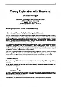
HipSpec’s operation is illustrated in Figure 1. We start by running QuickSpec on the program source file, which generates a list of conjectures. We also translate the program source code to a first-order theory using Hip. HipSpec maintains three sets of equations: active conjectures, which we still need to consider, failed conjectures, which we have already tried to prove but

QuickSpec

Conjectures

Open conjecture Timeout

Haskell Source

Induction (Hip)

Translation (Hip)

First-Order Theory

Theorem Prover Theorem

Extend theory

Fig. 1. An overview of HipSpec.

failed, and lemmas, which we have managed to prove. The first-order theory in Figure 1 consists of Hip’s translation of our program plus the current set of lemmas. Initially the active conjectures consist of all equations that QuickSpec found (even those that would have been removed by pruning), and the failed conjecture set and lemma set are empty. The main loop works as follows: 1. Pick a conjecture c from the active conjecture set (using a heuristic described below). 2. Check if c follows from the lemmas found so far by equational reasoning only. If so, discard c, and re-iterate. 3. Otherwise, ask Hip to prove the conjecture by induction, using definitions and previously proved lemmas as background theory. 4. If Hip succeeds, move c to the lemma set, and move some failed conjectures back to the active conjectures (based on a heuristic described below). 5. If Hip does not succeed within a set timeout, move c to the failed conjectures. The loop ends when the active conjecture set is empty. Picking the conjecture The performance of HipSpec completely depends on one heuristic: which active conjecture to try to prove next. Our current heuristics are rather crude; more sophisticated techniques are further work. Our basic strategy is to prove simpler equations before more complicated ones. We define simplicity as follows. A smaller term is simpler than a bigger term; if two terms have the same size, the term with more variables is simpler (because it might be more general). For example, (x+y)+z=x+(y+z) is simpler than (x+x)+y=x+(x+y). The simplicity of an equation t1 = t2 is determined by whichever of t1 and t2 is the most complex. We also take into account the call graph of the program. For example, if we are proving properties about the natural numbers, we prove as much as possible about + before starting on *, since * calls +. More precisely, when choosing which conjecture to prove next, we pick the one whose call graph is the smallest; if two conjectures have the same size call graph, we pick the simplest one.

Discarding trivial consequences It is quite expensive to send every conjecture to Hip to be proved, when we may have thousands of them. Luckily, QuickSpec has a lightweight theorem prover based on congruence closure. This prover can efficiently answer questions of the form “given these lemmas, can I prove this equation?”, replying either “yes” or “don’t know”. Whenever we pick a conjecture, we check if this prover can prove it from the current lemmas without induction. If so, we just discard it. This filters out most trivial conjectures that are provable without induction. Re-activating failed conjectures When we prove a lemma, we sometimes move some failed conjectures back to the active conjectures. HipSpec’s rule is to wait until the set of active conjectures is empty and then move all failed conjectures back to the active set, provided that at least one new lemma was proved since last attempting the conjecture. This guarantees termination. We have experimented with more elaborate heuristics in this step, eagerly adding failed conjectures back. These heuristics can help in certain examples, but so far none have been sufficiently general. Perhaps surprisingly, the simple method described above works well for all examples in this article. More sophisticated heuristics are further work.

3

Examples

This section gives examples of successful proofs and their related theory explorations, as well as an example showing some current limitations of our approach. 3.1

Rotating the length a of list

This simple property of the rotate function is surprisingly difficult to prove3 : prop_rotate xs = rotate (length xs) xs =:= xs The rotate function takes a natural number n and returns the list resulting from removing the n first elements and appending them to the end. Rotating a list by its length returns the original list. Although this property is very simple to state it is surprisingly hard to prove by mathematical induction, as it requires a generalised version to be proved, which implies prop_rotate. This generalisation itself can be proved by induction. Given the standard definitions of append, length and Peano numbers with successor S and zero Z, and the below definition of rotate, HipSpec finds and proves such a generalisation, and uses it to prove prop_rotate: rotate Z xs = xs rotate (S n) [] = [] rotate (S n) (x:xs) = rotate n (xs ++ [x]) 3

Here, =:= is HipSpec’s notation for equality.

The lemmas for which HipSpec needed induction are in Figure 2. Lemma (8 ) is the required generalisation, from which it proves prop_rotate, which follows as a special case when ys is the empty list. Notice that lemma (8 ) itself requires lemmas (1 ) and (2 ). A number of additional lemmas are also discovered, which are not of use in this particular proof, but could well be useful in other proofs. The whole process of theory exploration and the proof of prop_rotate took 17 seconds, with less than a second spent in QuickSpec and the rest of the time spent in various proofs of the generated equations. No (1 ) (2 ) (3 ) (4 ) (5 ) (6 ) (7 ) (8 ) (9 )

Conjecture xs++[] (xs++ys)++zs rotate n (rotate m xs) rotate (S n) (rotate m xs) rotate n [x] length (xs++ys) length (rotate n xs) rotate (length xs) (xs++ys) rotate (length xs) xs

= = = = = = = = =

Proved by xs xs xs++(ys++zs) xs rotate m (rotate n xs) n, m rotate (S m) (rotate n xs) xs, (3 ) [x] n length (ys++xs) xs, ys length xs n, (6 ) ys++xs xs, (1 ), (2 ) xs (8 )

Fig. 2. Properties generated and proved about the theory of lists with ++, rotate, and length. The third column shows which induction variables and lemmas were used.

As this proof requires both generalisation and lemma discovery it was identified in 2005 as an automated reasoning challenge beyond the capabilities of state-ofthe-art reasoning systems ([3], p. 77). We are not aware of any other theorem provers which prove this theorem fully automatically, without the help of usersupplied lemmas. 3.2

Nicomachus’ Theorem

Using Peano arithmetic, with standard definitions of addition and multiplication recursively on the first argument, we will try to get HipSpec to prove Nicomachus’ Theorem. This states that the sum of the n first cubes is the nth triangle number Pn Pn 2 squared: k=1 k 3 = ( k=1 k) . We define two functions: tri calculates triangle numbers and cubes n calculates the sum of the first n cubes. tri Z = Z tri (S n) = tri n + S n

cubes Z = Z cubes (S n) = cubes n + (S n*S n*S n)

Using these definitions, Nicomachus’ theorem is stated as follows: prop_Nicomachus x = cubes x =:= tri x * tri x When HipSpec is given the definitions of plus, multiplication, tri and cubes, it generates and proves (by induction) the properties listed in Figure 3 below, which takes 10 seconds. The properties are listed in the order they were proved.

No (1 ) (2 ) (3 ) (4 ) (5 ) (6 ) (7 ) (8 ) (9 )

Conjecture x+y x+(y+z) x*y x*(y*z) x*(y+y) (x*y)+(x*z) tri x*(y+y) tri x+tri x tri x*tri x

Lemmas used = = = = = = = = =

y+x (y+x)+z y*x (y*x)*z y*(x+x) x*(y+z) (x*y)*S x x+(x*x) cubes x

(1 ) (2 ) (1 ), (1 ), (1 ), (1 ), (1 ), (1 ),

(2 ), (2 ), (2 ), (2 ), (2 ), (2 ),

(3 ) (3 ), (4 ) (3 ) (3 ), (4 ), (6 ) (3 ) (3 ), (6 ), (8 )

Induction on x, y z x, y x, y y z x x x

Fig. 3. Properties proved about the theory with natural number addition, multiplication, triangle numbers (tri) and sum of cubes (cubes).

Pn In (8 ) the well-known identity k=1 k = n(n+1)/2 is proved, using previously proved lemmas. From this lemma HipSpec proves Nicomachus’ Theorem in (9 ). Due to the order in which HipSpec ends up proving the conjectures in this example, some unnecessary lemmas are included in figure 3, e.g. (5 ) and (7 ). 3.3

Insertion sort produces a sorted list

Currently, QuickSpec can only generate equational lemmas. To prove that, for example, insertion sort produces a sorted list requires conditional lemmas. We state this property as prop_sorted xs = sorted (isort xs) =:= True. In order to prove prop_sorted we need the conditional lemma sorted xs ==> sorted (insert x xs), where insert is the sorted list insertion function used by isort, but HipSpec only can only discover and prove the somewhat peculiar equations (lemmas 1-4 ) in Figure 4. HipSpec also discovers, but fails to prove, some additional properties (conjectures 5-9 ). For example, property (5 ), which states that insert is commutative in its first argument. These equations are not proved because they require conditional lemmas. Although not proved, QuickSpec has tested these equations and not found a counterexample. Hence, even a failed proof attempt may at least give some insight into the properties of the program. The runtime for this example was 8 seconds. No (1 ) (2 ) (3 ) (4 )

Conjecture x