INDUCTIVE CLUSTERING: AUTOMATING LOW-LEVEL SEGMENTATION IN HIGH RESOLUTION IMAGES Annie Chena, Gary Donovana, Arcot Sowmyaa, John Trinderb a
School of Computer Science and Engineering – (anniec, garyd, sowmya)@cse.unsw.edu.au b School of Surveying and Spatial Information Systems -
[email protected] University of New South Wales, Sydney 2052, Australia
KEY WORDS: Classification, clustering, inductive learning, RAIL, remotely sensed images, segmentation
ABSTRACT: In this paper we present a new classification technique for segmenting remotely sensed images, based on cluster analysis and machine learning. Traditional segmentation techniques which use clustering require human interaction to fine-tune the clustering algorithm parameters and select good clusters. Our technique applies inductive learning techniques using C4.5 to learn the parameters and pick good clusters automatically. The techniques are demonstrated on level 1 of RAIL, a hierarchical road recognition system we have developed.
1. INTRODUCTION Road detection and recognition from remotely sensed imagery is an important process in the acquisition and update of Geographical Information Systems (GIS) databases. Much effort has been put into the development of automated feature extraction methods, mainly in the areas of expert systems and advanced image analysis. In our previous papers we have described the RAIL/Recoil system (Singh, 1998; Sowmya, 1999; Trinder, 1999). RAIL (Road Recognition from Aerial Images using Inductive Learning) is a semi-automatic, multi-level, adaptive and trainable edge-based road recognition system intended to demonstrate the use of various Artificial Intelligence approaches in this area. Our goal is to implement several Artificial Intelligence algorithms to extract roads from remotely sensed images, thus demonstrating their viability for such problems. So far we have tested an inductive learner and two different clustering algorithms. Inductive learning is the process of generating a decision tree by having the computer "learn" rules, based on pre-classified examples provided to it. The resulting decision tree can then be used to classify new examples. One example application of an inductive learner to road recognition is to calculate thresholds, used for selecting edges that match road-sides. Traditionally these thresholds would be determined by human experts, but inductive learning can provide a more customized and locally applicable result. Clustering is an automated technique that involves sorting a set of data into groups, based on attributes of that data. Several different algorithms for accomplishing this have been proposed, including kNN and KMeans. In road extraction, clustering can be used, for example, to create a group of edges (or other image-level objects) that have similar shape, intensity, and so on, and hence form part of a road. Recently, we have developed a new inductive clustering framework. This uses inductive learning to improve the
results obtained from clustering, by learning the optimal clustering parameters for any situation. After the clustering is complete, the best clusters can be selected by using a decision tree. The details of this inductive clustering method are presented in this paper. Section 2 describes RAIL, inductive learning and clustering in more detail. In Section 3, we introduce the framework that combines inductive learning with clustering, and discusses the experimental components of that framework in detail. Finally, in Section 4 we present the results and evaluation of the framework. 2. BACKGROUND INFORMATION Our research builds upon the existing RAIL system, which includes components for inductive learning and clustering algorithms, amongst other features. In this section we will give some background information about these systems, to help readers understand our new inductive clustering method. The RAIL system has been used for many experiments in the past, including preliminary trials of Artificial Intelligence techniques in road-detection (Singh, 1998; Sowmya, 1999); a new junction recognition algorithm (Teoh, 2000a); and it was involved collaboratively in an expert system written in PROLOG (Trinder, 1998). 2.1 Rail In previous papers on the RAIL system (Singh, 1998; Sowmya, 1999; Trinder, 1999) we have described different aspects of its implementation. Briefly, RAIL is a multi-level edge-based road-extraction program, where straight edges are detected from a single-spectrum image using VISTA's implementation of the Canny operator (Pope, 1994). Level 1 joins pairs of opposite edges together, whilst Level 2 links the edge pairs together to make road sections. Levels 3 and 4 relate to intersection detection and integration, respectively. At each level, a different artificial intelligence technique can be applied, whether this be inductive learning, kNN clustering, KMeans clustering, or another method.
The International Archives of the Photogrammetry, Remote Sensing and Spatial Information Sciences, Vol. 34, Part XXX
At level 1, the objective is to join matching edges into edge pairs, or road segments. A road segment can be thought of as a pair of edges which are part of a road, and are opposite each other. The attributes, or properties, of such a road segment at RAIL Level 1 are listed in Table 1. Attributes / Relations Enclosed Intensity – Average intensity inside edge pair Parallel Separation – Average distance between edges Difference in spatial direction between edges Difference in gradient direction between edges Intensity difference (between inside & outside the segment)
Road Property Addressed Roads generally have high grayscale intensities
and each point from the data set is grouped into the closest cluster, one at a time. The method for determining the closest cluster depends on the particular algorithm. In KMeans, we measure the distance between the point and the center of every cluster, eventually choosing the cluster with the shortest distance. By contrast, kNN looks at the k nearest neighbors (i.e. the closest points from existing clusters), and the data point is placed in the cluster containing the most neighbors.
Road widths usually fall within a certain range
Once the clusters have been formed, clusters of interest are identified by visual inspection.
Roads generally appear as pairs of spatially parallel boundaries Road boundaries have opposite gradient directions Road appears brighter than its surroundings
A large number of experiments need to be run with different parameters in order to find the setting that produces the best result for a given problem. This whole clustering process requires a lot of hand tuning, to find a suitable algorithm, select the associated parameters, and finally pick out the useful clusters. In this paper we will suggest ways to automate this laborious process by applying inductive learning techniques to each of these stages.
Table 1. Description of road segment attributes Initial tests on our sample data set using cluster analysis revealed that the last three attributes do not usefully distinguish between different road segments. Since these attributes were ineffective, they were not used in further testing. To obtain the road segments (i.e. the Level 1 output) with normal clustering in RAIL, the following steps are followed: 1. Every possible edge pair is created by exhaustively pairing up every edge combination, and attributes are calculated for each edge pair. 2. These attributes are normalised and grouped into clusters using the chosen clustering algorithm and parameters. 3. Each cluster is visually compared with the original image. The cluster(s) with edge pairs that best match the road on the image are chosen as the set of road segments generated in Level 1. 4. Repeat from step 2 with different algorithm and parameters. 5. The road clusters from different clustering runs are compared, and the best one is chosen. Inductive clustering builds on this process, as described in Section 3. 2.2 Clustering As described above, clustering is the process of grouping a given set of data into separate clusters such that data points with similar characteristics will belong to the same cluster. There are many different algorithms for clustering, so we compared them to find the one most suitable for our application. In this paper we focus on the KMeans and kNN algorithms. Here we describe these algorithms briefly (see Weiss, 1991 for further details). The number of clusters (n) for these two algorithms is fixed in any given run. Since the best value of n is different for each data set, the user generally tries several values. Each cluster is initialized at a random position from the data set,
3. INDUCTIVE CLUSTERING FRAMEWORK Our inductive clustering framework has been designed to learn, from cluster descriptions what constitutes a good road cluster, and apply the learned knowledge to perform clustering automatically. The ultimate goal is to allow the system to take a new image, and deduce, from the characteristics of the image, the optimal algorithm and parameters to use. It will then automatically identify the road cluster for the user. This framework uses a multi-level learning strategy to tackle the process systematically at the following three stages (see Figure 1): Training Phase Testing Image with Reference model
Parameter Learning Rules for n Algorithm Learning Rules for algorithm Cluster Learning
Testing/Application Phase New Image without Reference model
Rules for
good cluster
Clustering
Figure 1. Inductive Clustering Framework Overview Parameter Learning: Learn the parameters that will give the best result for a given algorithm and image type. Parameters include n (the number of clusters) and k, in kNN clustering. Algorithm Learning: Learn which algorithm is most suitable for a given image type. The previous stage determines the parameters to use for each algorithm.
The International Archives of the Photogrammetry, Remote Sensing and Spatial Information Sciences, Vol. 34, Part XXX
Cluster Learning: We then learn to identify the road clusters by comparing their characteristics to known road and nonroad clusters. Inductive learning methods are used to derive rules at each level. These rules are combined at the end to allow a one step clustering process for extracting road clusters. We currently use the attribute-value learning program C4.5 (Quinlan, 1996) for the inductive learning process. To train our system we have to run a large number of experiments for each level. In order to automate each of these experiments we used a reference model for each data set, so that the evaluation of the results could be done automatically for each experiment. Since we used edge-based recognition algorithms, we were able to store the goal state as a simple set of edges. This reference model (or set) of edges was chosen by an experienced human operator. The quality of a cluster could then be measured by comparing the number of reference edges that have been chosen correctly. When compared with our old method of visually inspecting the image, this provides an objective (i.e. observer-independent) and quantifiable measure of the result. However there are still problems with this reference model system. The model deals with different objects than those created by the levels of RAIL, which leads to false positives. Moreover, this reference format models what the computer detects, not what is actually there in the real world. In consequence, our stated accuracies are mildly optimistic, at the least. A more suitable reference model would involve storing the actual shape of the road (e.g. its centerline and width). However, we have not yet implemented such a model. The measures we use to quantify our results are taken from (Harvey, 1999). They are percentage values, given by:
TP complete = size reference correct =
where
cxc = complete 3 × correct
(2)
Clearly, this measure is biased towards completeness. We also used a threshold to ensure that the cluster reached a minimum stage of completeness. These two tests can be expressed together as:
complete ≥ 80 % and cxc ≥ 95 × 10 6
(3)
The thresholds in Equation (3) are based upon empirical observations. 3.1 Parameter Learning In the parameter learning stage we want to deduce rules for the value of n (the number of clusters) to use on a given algorithm and image. The attributes that we use to learn clustering parameters are described in Table 2. This includes image characteristics, along with the clustering parameters we need to determine. Each set of attributes are classified as either good or bad. We then classify each setting as capable of generating good or bad road clusters by evaluating the best cluster produced by this setting with Equation (3). Name Size Algorithm n Classes
Description Number of edge pairs Clustering algorithm used Number of clusters Whether attributes produce a good or bad road cluster.
Value continuous KMeans, kNN [2, 30) good, bad
Table 2. Parameter learning attributes There are two phases in the parameter learning process, as shown in Figure 2.
(1)
TP size derived
TP = True positive size = Number of edges in the corresponding image
High completeness means that the cluster has covered the road edges well, whereas high correctness implies that the cluster does not contain many (incorrect) non-road edges. There is usually a trade off between the two measures, since a complete cluster is more likely to contain spurious non-road edges, and hence be less correct. It is computationally easier if there is only one criterion to distinguish between clusters. At Level 1 of RAIL, completeness is more important than correctness since we do not want to remove any information at this lower level. Hence our filtering criterion is:
Training Phase
Reference Model
Preprocessed Clustering Image Level Clusters attributes Image characteristics
Algorithm, n
Evaluate Good/bad C4.5 Rules
Testing/Application Phase New Image
Image attributes, algorithm
How many clusters n
Figure 2. Parameter Learning Experimental Design In the training phase, Level 1 RAIL attributes of the given image are calculated and used to cluster with different parameters. The clusters generated are evaluated against the
The International Archives of the Photogrammetry, Remote Sensing and Spatial Information Sciences, Vol. 34, Part XXX
reference model to determine which ones are "good". The inductive learner is then used to generate rules for choosing n in other, unseen, images. The purpose of the Testing/Application phase is obvious: we simply apply the generated rules on a new image to obtain the values of n to use for a given algorithm on that image. 3.2 Algorithm Learning The purpose of algorithm learning, as explained earlier, is to learn which algorithm to use for a given image type. The learning attributes here are image characteristics and the algorithm used (see Table 3). For each algorithm, the optimal n deduced from parameter learning was used. The algorithm that gives the best result on an image is classified as “good”, with the other being labeled “bad”. Name Size Algorithm
Description Number of edge pairs Clustering algorithm used
Classes
Whether the algorithm produced good or bad road clusters
Value continuous KMeans, kNN good, bad
Table 3. Algorithm Learning Attributes Algorithm learning has two phases of inductive learning, as shown in Figure 3. Training Phase
Reference Model
Preprocessed Clustering Image Level attributes
Clusters
3.3 Cluster Learning In cluster learning we want to deduce rules for identifying the road cluster of each clustering experiment. The learning attributes we have identified in Table 4 are cluster characteristics and image characteristics. We can classify each cluster as a good or bad road cluster by evaluating it against the reference model. Name Size Aspect ratio Area Centroid
Image attributes
continuous
Width max × Height max
continuous continuous
Good/bad
Rules
good, bad
Table 4. Cluster Learning Attributes Clustering experiments with different algorithms and parameters were run. All the clusters generated were evaluated against the reference model and classified based on the evaluation. The learning attributes from Table 4 together with the classification of each run were used in the inductive learner. This process is shown in Figure 4.
Training Phase
Reference Model
Preprocessed Image
Level attributes
Cluster
Clusters
Evaluate
Good/bad Analyze clusters
Best cluster’s performance
C4.5
New Image
Width max Height max
Evaluate
Algorithm
Testing/Application Phase
Value continuous
centre of the cluster Whether the cluster contains road edges.
Classes
Image character
Compare Performance Image character
Description Number of edge pairs
Cluster characteristics Algorithm
Testing/Application Phase New Image
Clustering
C4.5 Rules
Analyze clusters
Pick cluster
Pick method
Good clusters Method
Figure 4. Cluster Learning Experimental Design Figure 3. Algorithm Learning Experimental Design
4. RESULTS
The details of algorithm learning are similar to those of parameter learning. First, level 1 RAIL attributes of the given image were calculated and used to cluster with different algorithms. The clusters generated were evaluated against the reference model, and the algorithm producing the best road cluster was classified as “good”, with the other algorithm being labeled as “bad”. The learning attributes (see Table 3) together with the classification of each run were used to generate a decision tree for testing/application on new images.
The inductive clustering framework has been initially tested on two digital aerial images of a suburban area of France. These images have a ground resolution of 0.45m/pixel. One image contains 6481 edges (Figure 5a), and the other contains 1956 edges (Figure 5b).
The International Archives of the Photogrammetry, Remote Sensing and Spatial Information Sciences, Vol. 34, Part XXX
a) 4.1.1
Parameter Learning1
Rule 16: size > 7023 size 10 -> class good [70.7%] Rule 6: size > 1804 size 6 -> class good
[70.2%]
Rule 13: size > 6887 size 8 -> class good [61.2%] Rule 23: algorithm = kmeans size > 7146 n > 8 -> class good [61.2%] Rule 3: size > 1791 size 5 n class good
b)
[45.3%]
Rule 20: size > 7127 size 10 -> class good [45.3%] Rule 10:
Figure 5. Images used Since two images are not enough to learn from and test on, we divided these images into 5 sub-images, giving us 10 sets of edge pairs to experiment on. This subdivision was implemented by forming all possible edge pairs in an image, and calculating the RAIL level 1 attributes for those edge pairs. The resultant attributes were randomly split into 5 subsets, which were treated as independent sets for the purpose of testing. Clustering experiments were then run on each subset. Unbiased error rates were calculated using 5 fold cross validation (Weiss, 1991) for each stage of the framework (see Section 4.2). 4.1 Rules In this section we present the rules generated by inductive clustering on our two images. Note that the inductive clustering framework can be adapted to different applications and all sorts of images. However, the rules that we present below can only be applied to images with similar characteristics (e.g. resolution, complexity, etc.) to the ones we have used. We include them here to demonstrate the usefulness of our inductive clustering system on real images. Each rule identifies a partition of data via its learning attributes and gives a classification for that partition. The percentage after the classification indicates the accuracy of this rule when it is applied to the training data (note that this accuracy measure is optimistically biased).
size > 7094 n class bad
[97.2%]
size > 1806 size class bad
[96.6%]
n class bad
[95.1%]
Rule 8:
Rule 4:
Rule 2:
Default class: bad
Summary: For small images use n between 5 and 7. Use n greater than 8 for larger images, along with the KMeans algorithm. 4.1.2
Algorithm Learning
Rule 1: algorithm = knn -> class good [68.7%] Rule 2: algorithm = kmeans -> class bad [68.7%] Default class: good
Summary: kNN generally produces better results than KMeans.
1
To make the results clearer, some rules in the parameter learning section that did not involve n have been omitted.
The International Archives of the Photogrammetry, Remote Sensing and Spatial Information Sciences, Vol. 34, Part XXX
4.1.3
Cluster Learning
Rule 4: size > 8919 enclosed_intensity > 142.342 area > 1961.34 -> class good [80.9%] Rule 5: aspect_ratio > 1.43097 -> class bad [99.8%] Rule 1: area class bad [99.7%]
In the future we hope to improve the accuracy of our testing. One avenue for doing this is to develop a better reference model, addressing the inherent shortcomings of our current edge based one. We plan to train our system using a larger set of images in order to generate better rules. The evaluation measures used (cxc and complete) are handpicked and their thresholds set empirically. Automation of this process is a future goal. We also plan to extend this clustering framework to other levels of RAIL. 6. REFERENCES
Rule 3: enclosed_intensity class bad [99.0%] Default class: bad
Harvey, W. A., 1999. Performance Evaluation for Road Extraction. In: The Bulletin de la Société Française de Photogrammétrie et Télédétection, n. 153(1999-1):79-87
4.2 Evaluation
Pope, A. R., Lowe D. G., 1994. Vista: A Software Environment for Computer Vision Research. In IEEE Computer Vision and Pattern Recognition 1994, pp. 768772.
Table 5 shows the evaluation of the rules presented in the last section. We performed 5-fold cross validation on our data, in order to determine unbiased error rates.
Quinlan, J. R., 1996. C4.5: Programs For Machine Learning, San Mateo, California, Morgan Kaufmann Publishers.
This process involves randomly dividing the data into 5 partitions of approximately equal sizes. Leaving out one partition at a time, the remaining data is used to generate a decision tree, which is tested on the 5th partition. Given some assumptions, the average of the 5 error rates is then the error rate for the decision tree. This produces an unbiased measure.
Singh, S., Sowmya, A., 1998. RAIL: Road Recognition from Aerial Images Using Inductive Learning. In: The International Archives of the Photogrammetry, Remote Sensing and Spatial Information Sciences, Vol. XXXII, Part 3/1, pp. 367-378
Summary: Road clusters have an enclosed intensity greater than 142.342 and area greater than 1961.34.
The rules induced for parameter learning, algorithm learning and cluster learning show 94.1%, 77.4% and 99.2% accuracy respectively. Stats data size training Fold testing 1 accuracy training Fold testing 2 accuracy training Fold testing 3 accuracy training Fold testing 4 accuracy training Fold testing 5 accuracy Error rate
Parameter 521 429 17 96.8 % 413 114 91.2 % 405 102 94.1 % 407 103 95.1 % 430 109 93.6 % 94.1%
Algorithm 52 39 10 70 % 43 9 88.9 % 40 12 75 % 42 10 90 % 44 11 63.3 % 77.4%
Cluster 4945 3985 645 99.5 % 3953 727 98.9 % 3967 669 99.6 % 3925 3925 98.9 % 3950 726 98.9 % 99.2 %
Table 5. Evaluation 5. CONCLUSION AND FUTURE WORK In this paper we have introduced a way of automating clustering for road classification using inductive learning techniques. We have implemented and tested this concept on our RAIL system, and preliminary results are encouraging.
Sowmya, A., Singh, S., 1999. RAIL: Extracting road segments from aerial images using machine learning, In: Proc. ICML 99 Workshop on Learning in Vision. pp. 8-19. Teoh, C.Y., Sowmya, A., 2000a. Junction Extraction from High Resolution Images by Composite Learning. In: The International Archives of the Photogrammetry, Remote Sensing and Spatial Information Sciences, Amsterdam, Netherlands, Vol. XXXII, Part B3, pp882-888. Teoh, C.Y., Sowmya, A., Bandyopadhyay S., 2000b. Road Extraction from high resolution images by composite learning, In: Proceedings of International Conf. Advances in Intelligent Systems: Theory and Applications, Amsterdam, Netherlands, pp308-313. Trinder, J. C., Nachimuthu, A., Wang, Y., Sowmya, A., Singh, A., 1999. Artificial Intelligence techniques for Road Extraction from Aerial Images. In: The International Archives of the Photogrammetry, Remote Sensing and Spatial Information Sciences. Vol. XXXII, Part 3-2W5, pp. 113-118 Trinder, J. C., Wang, Y., 1998. Automatic 4D Feature Extraction from Aerial Imagery. In: Digital Signal Processing. 8, pp. 215-224 Weiss, S., Kulikowski, C., 1991. Computer Systems That Learn, San Francisco, California, Morgan Kaufmann Publishers.