Automating the construction of CBR systems using Kernel Methods Colin Fyfe Applied Computational Intelligence Research Unit The University of Paisley High Street, Paisley, PA1-2BE, UK
Juan M. Corchado Department of Languages and Computing Systems University of Vigo, Campus Universitario, 32004, Ourense, Spain
Email:
[email protected]
Email:
[email protected]
Abstract Instance based reasoning systems and in general case based reasoning systems are normally used in problems for which it is difficult to define rules. Although case-based reasoning methods have proved their ability to solve different types of problems, there is still a demand for methods that facilitate their automation during their creation and the retrieval and reuse stages of their reasoning circle. This paper presents one method based on Kernels, which can be used to automate some of the reasoning steps of instance-based reasoning systems. Kernels were originally derived in the context of Support Vector Machines, which identify the smallest number of data points necessary to solve a particular problem (e.g. regression or classification). Unsupervised Kernel methods have been used successfully to identify the optimal instances to instantiate an instance-base. The efficiency of the Kernel model is shown on an oceanographic problem.
1.- Introduction Although case based reasoning (CBR) systems have been successfully used in several domains such as: diagnosis, prediction, control and planning [1,2], there are no standard techniques to automate their
1
construction. Arguably feature identification, case representation, similarity metric selection, case discovery and general adaptation rule learning are the most difficult aspects to automate in these type of systems [3]. This paper presents a method that can be used to tackle this problem, which can substantially facilitate the automatic construction of such systems. Automating, in this context, means that this method can be easily used to construct retrieval and adaptation mechanism for instance based easoning (IBR) systems.
Kernel models were first developed as part of the method of Support Vector Machines [4]. Support Vector Machines attempt to identify the minimum number of data points (the support vectors) which are necessary to solve a particular problem to the required accuracy. Kernels have been successfully used in unsupervised structure investigation [5,6]. In this paper, we will investigate the use of Kernel methods to identify cases, which will be used in a case based reasoning system.
Kernel methods can be used in case based reasoning systems when cases can be represented in the form of numerical feature vectors. This is normally the case in most of instance based reasoning systems (IBR) [7,8]. The features that characterise Kernel models can be used to identify prototypical cases, to identify cases that are similar to a given one and to reuse cases. Large case-bases may have negative consequences for the performance of the CBR systems. This has been shown in several projects such as INRECA [9] and STEB [8]. The ability of the Kernel methods presented in this paper to select prototypical cases and to identify those cases that are already represented by these prototypes can be used to successfully prune the case-base without losing valuable information.
2
This paper is structured as follows: first CBR systems are reviewed; then Kernel Principal Component Analysis is presented, a refinement involving sparsification of the vectors/cases is derived, and this method's abilities is demonstrated on synthetic data sets. Finally we show how this approach has been used in a realworld system to forecast thermal time series in real time.
2.- Case/Instance -based Reasoning Systems A case-based reasoning system is a model of human reasoning [10]. The idea behind CBR is that people rely on concrete previous experiences when solving new problems. This fact can be tested on any day to day problem by simple observation or even by psychological experimentation [11]. Since the CBR model was first proposed, it has proved successful in a wide range of application areas [1,2,13,14].
A case-based reasoning system solves new problems by adapting solutions that were used to solve old problems [15]. The case base holds a number of problems with their corresponding solutions. Once a new problem arises, the solution to it is obtained by retrieving similar cases from the case base and studying the similarity between them. A CBR system is a dynamic system in which new problems are added to the case base, redundant ones are eliminated and others are created by combining existing ones.
CBR systems record past problem solving experiences and, by means of indexing algorithms, retrieve previously stored cases, along with their solutions, and match them and adapt them to a given situation, to generate a solution. The intention of the CBR system is to abstract a solution from the knowledge stored in the case-base in the form of cases. All of these actions are self-contained and can be represented by a cyclical
3
sequence of processes in which human intervention may be needed. A case-base reasoning system can be used by itself or as part of another intelligent or conventional system. CBR systems are especially appropriate when the rules that define a knowledge domain are difficult to obtain or the number and the complexity of the rules affecting the problem are too large for the normal knowledge acquisition problem.
A typical CBR system is composed of four sequential steps which are recalled every time that a problem needs to be solved [1,13,16]: 1. Retrieve the most relevant case(s), 2. Reuse the case(s) to attempt to solve the problem, 3. Revise the proposed solution if necessary, 4. Retain the new solution as a part of a new case.
Each of the steps of the CBR life cycle requires a model or method in order to perform its mission. The algorithms selected for the retrieval of cases should be able to search the case base and to select from it the most similar problems, together with their solutions, to the new problem. Cases should therefore represent, accurately, problems and their solutions. Once one or more cases are identified in the case base as being very similar to the new problem, they are selected for the solution of this particular problem. These cases are reused using a predefined method in order to generate a proposed solution (i.e. normally using an adaptation technique). This solution is revised (if possible) and finally the new case (the problem together with the obtained solution) is stored. Cases can also be deleted if they prove to be inaccurate; they can be merged together to create more generalised ones and they can be modified.
4
CBR systems are able to utilise the specific knowledge of previously experienced problem situations rather than making associations along generalised relationships between problem descriptors and conclusions or relying on general knowledge of a problem domain such as rule-based reasoning systems. CBR is an incremental learning approach because every time that a problem is solved a new experience can be retained and made immediately available for future retrievals.
The nature of the problem and the expertise of the CBR designers determine how the CBR should be built. Although there are will known standard metrics for each of the steps of the CBR cycle [1,3,13,16] there are only a few techniques that can facilitate the automation of the construction of CBR systems [3]. This paper presents a method to do both this and to automate the process of case retrieval and adaptation in problems of a numeric nature.
According to Aamodt and Plaza [16] there are five different types of CBR systems, and although they share similar features, each of them is more appropriate for a particular type of problem: exemplar based reasoning, instance based reasoning, memory-based reasoning, analogy-based reasoning and typical case-based reasoning.
Those CBR systems that focus on the learning of concept definitions are normally referred to as being exemplar-based. In the literature there are different views of concept definition [17]. A concept is defined extensionally as the set of its examples. PROTOS [18] is an example of this type of CBR systems. In this
5
case, solving a problem requires finding the right class for an unclassified exemplar. The class solution of the most similar retrieved case is the problem case solution. Instance-based reasoning (IBR) can be considered as exemplar-based reasoning is useful in highly syntactic problem [16]. This type of CBR system focuses on problems in which there are a large number of instances which are needed to represent the whole range of the domain and where there is a lack of general background knowledge. The case representation can be made with feature vectors and the phases of the CBR cycle are normally automated as much as possible, eliminating human intervention This paper focuses on the automation of IBR systems with Kernel methods which are appropriate because of their numerical characteristics.
3.- Kernel Methods The use of Radial Kernels has been derived from the work of Vapnik [4], Burges [19] etc. in the field of Support Vectors Machines. Support Vector Machines for regression for example, perform a nonlinear mapping of the data set into some high dimensional feature space in which we may then perform linear operations. Since the original mapping was nonlinear, any linear operation in this feature space corresponds to a nonlinear operation in data space.
We first review recent work on Kernel Principal Component Analysis (KPCA) which has been the most frequently reported linear operation involving unsupervised learning in feature space [5,6,20]. Then it is shown why the basic KPCA method is not appropriate for the selection of instances for an IBR system. We therefore use a sparsification of the KPCA method which is appropriate for this type of problems.
6
3.1.- Kernel PCA This section shows that sample Principal Component Analysis (PCA) may be performed on the samples of a data set in a particular way which will be useful in the performance of PCA in the nonlinear feature space.
PCA finds the eigenvectors and corresponding eigenvalues of the covariance matrix of a data set. Let χ = {x 1 ,..., x M } be iid (independent, identically distributed) samples drawn from a data source. If each xi is n-
dimensional, ∃ at most n eigenvalues/eigenvectors. Let C be the covariance matrix of the data set; then C is n × n. Then the eigenvectors, ei, are n dimensional vectors which are found by solving
Ce = λe
(1)
where λ is the eigenvalue corresponding to e. We will assume the eigenvalues and eigenvectors are arranged in non-decreasing order of eigenvalues and each eigenvector is of length 1. We will use the sample covariance matrix as though it was the true covariance matrix and so
C≈
1 M
M
∑x x j
T j
(2)
j =1
Now each eigenvector lies in the span of χ ; i.e. the set χ = {x1 ,..., x M } forms a basis set (normally overcomplete since M > n) for the eigenvectors. So each e i can be expressed as
7
e i = ∑ α ij x j
(3)
j
If we wish to find the principal components of a new data point x we project it onto the eigenvectors previously found: the first principal component is (x.e 1), the second is (x.e 2), etc. These are the coordinates of x in the eigenvector basis. There are only n eigenvectors (at most) and so there can only be n coordinates in the new system: we have merely rotated the data set.
Now consider projecting one of the data points from χ on the eigenvector e 1; then
x k e1 = x k .∑ α 1j x j = a 1 .∑ x k x j j
(4)
j
Now let K be the matrix of dot products. Then K ij = xi x j .
Multiplying both sides of (1) by xk we get
x k Ce 1 = λ e1 .xk
(5)
and using the expansion for e 1, and the definition of the sample covariance matrix, C, gives
8
1 2 K a 1 = λ1 Ka 1 M
(6)
Now it may be shown [5] that all interesting solutions of this equation are also solutions of
Ka 1 = Mλ1a 1
(7)
whose solution is that α 1 is the principal eigenvector of K.
Now so far we have only found a rather different way of performing Principal Component Analysis. But now we preprocess the data using Φ : χ → F . So F is now the space spanned by Φ (x1 ),...,Φ (x M ) . The above arguments all hold and the eigenvectors of the dot product matrix K ij = (Φ( x i ). Φ(x j )) are the equivalent vectors in the feature space. But now the Kernel Trick : provided we can calculate K we don't need the individual terms Φ (x i ) .
As an example of how to create the Kernel matrix, we may use Gaussian kernels so that
K ij = ( Φ( xi ).Φ (x j )) = exp( − ( x i − x j ) 2 ( 2σ 2 ))
(8)
This kernel has been shown [5] to satisfy the conditions of Mercer's theorem and so can be used as a kernel for some function Φ (.) . One issue that we must address in feature space is that the eigenvectors should be of unit length. Let vi be an eigenvector of C. Then vi is a vector in the space F spanned by Φ (x1 ),...,Φ (x M ) and
9
so can be expressed in terms of this basis. This is an at most M-dimensional subspace of a possibly infinite dimensional space which gives computational tractibility to the kernel algorithms. Then
M
v i = ∑α ij Φ(x j )
(9)
j =1
for eigenvectors vi corresponding to non-zero eigenvalues. Therefore v Ti v i
= =
M
∑α
i j
Φ (x j ) T Φ( x k )α ki
∑α
i j
K jkα ki
j ,k =1 M j ,k =1
= a i .( Ka i ) = λ i a i .a i
Now a i are (by definition of the eigenvectors of K) of unit magnitude. Therefore since we require the eigenvectors to be normalised in feature space, F, i.e. v Ti v i = 1 , we must normalise the eigenvectors of K, a i , by dividing each by the square root of their corresponding eigenvalues.
Now we can simply perform a principal component projection of any new point x by finding its projection onto the principal components of the feature space, F. Thus
M
M
j =1
j =1
v i .Φ(x) = ∑ α ij Φ (x j ).Φ( x) = ∑ α ij K ( x j , x)
(10)
10
Figure 1 shows the clustering ability of Kernel PCA with a Gaussian Kernel. The data set comprises 3 sets each of 30 points each of which is drawn from a Gaussian distribution. The centres of the three Gaussians are such that there is a clear separation between the clouds of points. The figure shows the contours of equal projection onto the first 8 KPCA directions. Note that linear PCA would only be able to extract 2 principal components; however because the kernel operation has moved us into a high dimensional space in a nonlinear manner, there may be up to 90 non-zero eigenvalues. The three clusters can be clearly identified by projecting the data points onto the first two eigenvectors. Subsequent Kernel Principal Components split the clusters into sections.
However Figure 2 shows the components of the eigenvectors in feature space. We see why the first two projections were so successful at identifying the three clusters but we note that there is a drawback to the method if we were to use this method to identify cases: each eigenvector is constructed with support from projections of very many points. What we really wish is to identify individual points in terms of their importance. This issue has previously been addressed in [6] using a number of heuristics. In this paper we use a novel sparsification of the Kernel PCA method.
11
Figure 1: The 3 clusters data set is shown as individual points. The co n t o u r s are contours of equal projection on the respective Principal Comp o n e n t s . The first two principal components are sufficient to differentiate between the three clusters; the others slice the clusters internally and have much less variance associated with them.
Figure 2: The first eight eigenvectors found (each vector is represented in a horizontal line) by Kernel PCA. Each eigenvector has elements from every data point.
12
3.2.- Sparse Kernel Principal Component Analysis It has been suggested [20] that we may reformulate the Kernel PCA problem as follows: let the set of permissible weight vectors be
M
V = {w : w = ∑ α i Φ (x i ), with w i =1
2
= ∑ α i α j K ( xi , x j ) ≤ 1}
(11)
i, j
Then the first principal component is
v1 = arg max v∈V
1 M
M
∑ v.Φ (x )
2
i
i =1
(12)
for centred data. This is the basic KPCA definition which we have used above. Now we may ask whether other sets of permissible vectors may also be found to be useful. Consider
M
VLP = {w : w = ∑α i Φ(x i ), with ∑ α i ≤ 1} i=1
(13)
i
This is equivalent to a sparsity regulariser used in supervised learning and leads to a type of kernel feature analysis
v1 = arg max v∈VLP
1 M
M
∑ v.Φ(x ) i
2
(14)
i =1
13
We may think that subsequent "principal vectors" can be found by removing this vector from further consideration and ensuring that the subsequent solutions are all orthogonal to the previously found solutions. However as we shall see there are problems in this simple solution. [20] point out that this system may be generalised by considering the lp norm to create permissible spaces
M
VP = {w : w = ∑ α i Φ( x i ), with ∑ α i ≤ 1} i =1
(15)
i
3.3.- Solutions and Problems Smola et al. [20] have shown that the solutions of
v1 = arg max v∈Vp
1 M
M
∑ v.Φ( x )
2
(16)
i
i =1
are to be found at the corners of the hypercube determined by the basis vectors, Φ( x i ) . Therefore all we require to do is find the element x k defined by
M
M
x k = arg max ∑ Φ (x k ).Φ (x i ) = arg max ∑ K k i xt ∈ χ
i =1
2
xt ∈ χ
2
(17)
i =1
which again requires us only to evaluate the kernel matrix. 14
So the solution to finding the "First Principal Component" using this method is exceedingly simple. However, subsequent PCs cause us more concern. Consider first the "naive" solution which is simply to remove the winner of the first competition from consideration and then repeat the experiment with the remainder of the data points. However these data points may not reveal interesting structure: typically indeed the same structure in input space (e.g. a cluster) may be found more than once. In the data set to be consid ered in this paper, this indeed happens. Indeed the first 10 Kernel Principal Components are in fact all from the same cluster of data and are highly redundant.
An alternative is to enforce orthogonality using a Gram Schmidt orthogonalisation in feature space. Let v1 = Φ1 ( x i ) for some i. Then
Φ 2 (x j ) = Φ 1 (x j ) − = Φ 1 (x j ) −
2
(Φ (x ).v )
2
K (x j , x i )
v1 v1 v1 v1
1
j
1
where we have used Φ1 to denote the nonlinear function mapping the data into feature space and Φ 2 to denote the mapping after the orthogonalisation has been performed i.e. the mapping is now to that part of the feature space orthogonal to the first Principal Component. Using the same convention with the K matrices gives
15
v v Φ 2 (x j ).Φ 2 (x k ) = Φ1 (x j ) − 12 K1 (x j , x i ). Φ 1(x k ) − 12 K 1 (x k , x i ) v1 v1 2 K1 (x j , x i )K 1(x k , x i ) K1 (x j , xi )K 1(x k , x i ) = K1 (x j , x k ) − + 2 2 v1 v1
i.e. K 2 (x j , x k ) = K 1 (x j , x k ) −
K 1 (x j , x i )K 1 (xk , xi ) K1 ( xi , xi )
which can be searched for the optimal values. The method can clearly be applied recursively and so
K i +1 (x j , x k ) = K i (x j , x k ) −
K i (x j , xi )K i (x k , x i ) K i (x i , x i )
for any time instant i+1.
One difficulty with this method is that we can be (and typically will be) moving out of the space determined by the norm. Smola et al. [20] suggest renormalising this point to move it back into Vp. This can be easily done in feature space and both the orthogonalisation and renormalising can be combined into K i +1 (x j , xk ) =
K i (x j , x k )K i ( xi , x i ) − K i (x j , x i )K i (x k , xi )
K ( xi , x i ){ K i ( xi , x i ) + K i (x j , x k )}{ K i (x i , xi ) − K i (x j , x i )} 3 i
which is a somewhat cumbersome expression and must be proved to be a valid kernel. In this paper we do not perform this step having found it to be unnecessary. We will demonstrate that finding the maximal projection corner from the remainder after orthogonalisation is a very good method for selecting instances from an IBR system.
16
4.- IBR for oceanographic real-time forecasting A forecasting system capable of predicting the temperature of the water ahead of an ongoing vessel in real time has been developed using a IBR system [8,21]. An IBR system was selected for its capacity of handling huge amounts of data, of adapting to the changes in the environment and to provide real time forecast. The cyclic IBR process shown has been inspired by the ideas described by Aamondt and Plaza [16].
Knowledge Acquisition
New Instance
Retrieve Instances
M instances
X Instances
Learned ANN Architecture & prop. forecast
ANN weights & centres,
Retain
Final Forecast
Instance Base
Reuse ANN weights & centres
General Knowledge Confidence limits
Review
Proposed Forecast
Figure 3: IBR system architecture.
In Figure 3, shadowed words (together with the dotted arrows) represent the four steps of a typical IBR life cycle, the arrows together with the word in Italic represent data coming in or out of the instance-base
17
(situated in the center of the diagram) and the text boxes represent the result obtained by each of the four stages of the IBR life-cycle. Solid lines show data flow and dotted lines show the order in which the processes that take part in the life cycle are executed.
Data are recorded in real time by sensors in the vessels and satellite pictures are received weekly. A Knowledge Acquisition module is in charge of collecting, handling and indexing the data in the instancebase. Once the real-time system is activated on an ongoing vessel, a new instance is generated every 2 km using the temperatures recorded by the vessel during the last 40km. This new instance is used to retrieve m cases from a collection of previous cases using a number of K-nearest neighbour metrics. The m-retrieved instances are adapted by a neural network during the reuse phase to obtain an initial (proposed) forecast. Though the revision process, the proposed solution is adjusted to generate the final forecast using the confidence limits from the knowledge base. Learning (retaining) is achieved by storing the proposed forecast and knowledge (ANN weights and centers) acquired by the ANN after the training and case adaptation. A complete description of this system can be obtained in [8,21].
This IBR system has been successfully tested and it is presently operative in several oceanographic vessels [21]. Improving this system has been our challenge and this section will outline the modifications that has been done to it with the intention of demonstrating that the Kernel methods can provide successful results and automate the retrieval of instances. The following tables shows the changes that have been done in the IBR system for real time oceanographic forecasting.
18
STEP
Operating IBR system
Modifications and improvements
Retrieval of instances
K-nearest neighbour algorithms
Kernel methods
Reuse of instances
Radial Basis Function Network
Unsupervised Kernel methods
Learning of instances
Radial Basis Function Network
Kernel methods
Pruning Metrics
Table 1: Changes in the IBR system for real time oceanographic forecasting
Table 1 outlines the changes made to the original system. The first column of the table indicates in which steps of the IBR life cycle the changes have been made, the second column indicates the method originally used (and now eliminated) and column three indicates which methods have been included in the system. The changes indicated in table 1 have been introduced with the intention of developing a robust model, based on a technology easy to implement and that can automate the process of defining the retrieval, reuse and learning steps of the IBR system. We now present the structure of a case and indicated how the kernel methods have been used in the three mentioned IBR Steps.
4.1. - The Instance
Each stored instance contains information relating to a specific situation and consists of an input profile (i.e. a vector of temperature values) together with the various fields shown in Table 2.
19
Instance Field
Explanation
Identification
unique identification: a positive integer in the range 0 to 64000
Input Profile, I
A 40 km temperature input vector of values Ij, (where j = 1, 2, … 40) Representing the structure of the water between the present position of the vessel and its position 40 km back.
Output Value, F
A temperature value representing the water temperature 5 km ahead of the present location
Time
Time when recorded (although redundant, this information helps to ensure fast retrieval)
Date
Date when the data were recorded (included for the same reasons as for the previous field).
Location
Geographical co-ordinates of the location where the value I 40 (of the input profile) was recorded.
Orientation
Approximate direction of the data track, represented by an integer x, (1 ≤ x ≤12).
Retrieval Time
Time when the instance was last retrieved.
Retrieval Date
Date when the instance was last retrieved.
Retrieval Location
Geographical co-ordinates of the location at which the instance was last retrieved.
Average Error
Average error over all forecasts for which the instance has been used during the adaptation step.
Table 2. Instance structure.
A 40 km data profile has been found to give sufficient resolution to characterise the problem instance. The parametric features of the different water masses that comprise the various oceans vary substantially, not only geographically, but also seasonally. Because of these variations it is therefore inappropriate to attempt to maintain an instance base representing patterns of ocean characteristics on a global scale; such patterns, to a large extent, are dependent on the particular water mass in which the vessel may currently be located.
20
Furthermore, there is no necessity to refer to instances representative of all the possible orientations that a vessel can take in a given water mass. Vessels normally proceed in a given predefined direction. So, only instances corresponding to the current orientation of the vessel are normally required at any one time.
4.2 Creating the Instance-base with Sparse Kernel Principal Component Analysis We use the Sparse KPCA method described in Section 3.3 to create a small number of cases which best typify the data set. For pedagogical purposes, we illustrate the method on a small sample of cases: we choose 150 cases of the oceanographic temperature data described above. The data set is illustrated in Figure 4.
21
Figure 4: The data set comprises 50 points from each of three water masses. The left diagram shows the first element from each instance; the right plots the first element from each instance against the value the instance is attempting to predict. The water masses are clearly visible from the data.
The left diagram shows the first element from each instance; the right plots the first element from each instance against the value the instance is attempting to predict. The water masses are clearly visible from the data and the strong structure of the data set leads us to believe that there should be much fewer than 150 significant instances.
We have experimented with a number of Sparse KPCA components and illustrate one example the reduced set shown in Figure 5: we show the rows of the K matrix associated with the first 15 PCA vectors. These most important vectors (instances) were 122, 92, 83, 66, 73, 60, 106, 32, 78, 98, 53, 70, 36, 63 and 54: two from the group 101 – 150, eleven from 51-100 and two from 1-50. We can see from the rows of the K matrix (Figure 5) that the data set is well covered by these 15 points. It is unsurprising that there are most points from the central group as it contains most structure. We now have a method for identifying the most important vectors (prototypical instances) in the data set but there still remains the question of how accurate predictions will be if they only are based on a small set of data samples.
22
Figure 5: The 15 rows of the K matrix associated with the first “Kernel Principal Components” when using deflationary method
4.3.- Retrieving Instances from the Instance Base Any new data point x may be associated with a particular instance by creating its Kernel projection onto the previously found important vectors (prototypical instances) and finding the maximally valued projection. Given the relatively small number of important vectors, this is a very fast operation. For example with Gaussian kernels, we need only evaluate K ( x, x j ) = exp( −( x − x j ) / σ ) for all xj in the set of stored cases. 2
It is simple to implement a vigilance parameter so that if the projection on the best instance is too small, the point is added to the instance base.
4.4.- Forecasting with the Instance-base Reasoning System Several experiments have been carried out to illustrate the effectiveness of the IBR system, which incorporates the Kernel models. Experiments have been carried out using data from the Atlantic Meridian Transept (AMT) Cruise 4 [21]. We show in Figure 6 the errors on our original data set of 150 instances of taking the forecast temperature of the retrieved instance and subtracting the actual temperature of the case. In this experiment we
23
used 20 instances and so a substantial reduction in instances was achieved. The mean absolute error, when forecasting the temperature of the water 5 Km ahead of an ongoing vessel, along 10000 km (form the UK to the Falkland Island) was 0.0205 ºC which compares very favourably with the inicial Instance based reasoning system and other previous methods [8,21].
We can also see that the first and second data sets (of 50 samples each) are much more difficult to forecast than the third. The difficulty of the first water mass was not obvious from a visual inspection of the data but becomes obvious when one considers the points found to be important in constructing the instance base.
Figure 6: The error on the 150 points. We see that the last group of 50 data points is the easiest to predict. The first group is surprisingly difficult.
5.- Conclusion
24
We have demonstrated a new technique for identification of the important instances, which could be used to construct instance based reasoning systems. The basis of the method is a sparsification of the new method of Kernel principal component analysis. The sparsification leads to an extremely simple algorithm in feature space which has been shown to give extremely accurate results on an exemplar forecasting task: our results of 0.0205 ºC error are among the best we have ever achieved on this data set and we have done so with a very much reduced instance base [8,21]. Of interest too is the fact that the method allows investigation of the nonlinear projection matrix K that readily reveals when a new body of water is reached. This is very important in the identification of fronts in these large bodies of water particularly since such fronts have an extremely adverse effect on underwater communications.
The retrieval of the best matching instance is a very simple operation and presents no major computational obstacles. The whole system may be used with any number-based set of data; an area of ongoing research is the derivation of metrics which are appropriate for non-numeric data. One of the major advantages of the supervised Kernel method, support vector machines, is the automatic detection of relevancy and the pruning of data which is not essential to determine e.g. a classification or regression plane. We have presented one method here for sparsification of the instance base and are currently investigating other techniques based on Kernels that could have similar consequences. Such methods are both advantageous in the creation of and retrieval from instance bases but are also important in their own right in the unsupervised investigation of data sets using Kernel methods.
25
Acknowledgement The contributions of N. Rees and Prof. J. Aiken at the Plymouth Marine Laboratory in the collaborative research presented in this paper are gratefully acknowledged.
References [1] Watson I. (1997) Applying Case-Based Reasoning: Techniques for Enterprise Systems. Morgan Kaufmann. [2] López de Mántaras R. and Plaza E. (1997). Case-Based Reasoning: an overview. AI Communications 10. pp. 21-29. IOS Press. [3] Anand S. S., Aamodt A. and Aha D. W. (eds.) (1999) Automating the Construction of Case Based Reasoners. Workshop ML-5, IJCAI 99. [4] Vapnik, V. (1995) The nature of statistical learning theory, Springer Verlag. [5] Scholkopf, B., Mika, S., Burges, C., Knirsch, P., Muller, K.-R., Ratsch, G. and Smola, A. (1999) Input space vs feature space in kernel-based methods. IEEE Transactions on Neural Networks, 10:10001017. [6] Fyfe, C., MacDonald, D., Lai, P.L., Rosipal, R., and Charles, D. (2000) Unsupervised Learning with Radial Kernels in Recent Advances in Radial Basis Functions, Editors R. J. Howlett and , Elsevier, 2000. [7] Lees, B. and Corchado, J. (1999) Integrated case-based approach to problem solving. In: Lecture Notes in Artificial Intelligence 1570, XPS-99: Knowledge-Based Systems - Survey and Future Directions, edited by Frank Puppe, Springer, Berlin, pp. 157-166.
26
[8] Corchado J. M. and Lees B. (2000) Adaptation of cases for case-based forecasting with neural network support., S.K Pal, T.S. Dillon and D.S. Yeung (Eds.), Soft Computing in Case Based Reasoning", Springer Verlag, London, 2000 (In press). [9] Wilke W. y Bergmann R. (1996). Incremental Adaptation with the INRECA- System. ECAI 1996 Workshop on Adaptation in Case-Based Reasoning. [10] Joh D. Y. (1997). CBR in a Changing Environment. Case Based Reasoning Research and Development. ICCBR-97. Providence, RI, USA. [11] Klein G. A. and Whitaker L. (1988) Using Analogues to Predict and Plan. Proceedings of a Workshop on Case-Based Reasoning. pp. 224-232. [12] Ross B. H. (1989) Some psychological results on case-based reasoning. K. J. Hammond, Proceedings of the Case-Based Reasoning Workshop. pp. 318-323. Pensacola Beach, Florida. Morgan Kaufmann. [13] Kolodner J. (1993) Case-Based Reasoning. San Mateo. CA, Morgan Kaufmann. [14] Pal S.K, Dillon T.S. and Yeung D.S. (Eds.) (2000) Soft Computing in Case Based Reasoning, Springer Verlag, London (In press). [15] Riesbeck C. K. and Schank R. C. (1989) Inside Case-Based Reasoning. Lawrence Erlbaum Ass. Hillsdale. [16] Aamodt, A. and Plaza, E. (1994) Case-Based Reasoning: foundational Issues, Methodological Variations, and System Approaches, AICOM, Vol. 7 No. 1, March. [17] Smith E. and Medin D. (1981) Categories and concepts. Harvard University Press.
27
[18] Porter B. and Bareiss R. (1986) PROTOS: An experiment in knowledge acquisition for heuristic classification tasks. Proceedings First International Meeting on Advances in Learning (IMAL). Les Arcs, France. pp. 159-174. [19] Burges, C., (1998) A tutorial on support vector machines for pattern recognition. Data Mining and Knowledge Discovery, 2(2):121-167. [20] Smola, A. J., Mangasarian, O.L., and Scholkopf, B (1999) Sparse kernel feature analysis. Technical Report 99-04, University of Wisconsin, Madison. [21] Corchado J. M. (2000) Neuro-symbolic Model for Real-time Forecasting Problems. Thesis Dissertation. University of Paisley. January.
28