Automation of Structured Overset Mesh Generation for Rocket ...

AIAA-2009-3993 19th AIAA Computational Fluid Dynamics Conference

Automation of Structured Overset Mesh Generation for Rocket Geometries Shishir Pandya∗, William Chan† NASA Ames Research Center, M.S. T-27B, Moffett Field, CA 94035

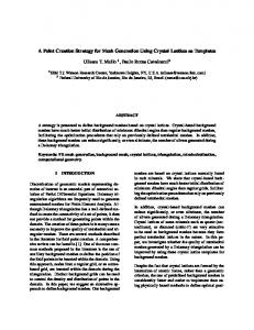
James Kless‡ ELORET, M.S. T-27B, Moffett Field, CA 94035 Aerodynamic characterization in the ascent phase is one of the necessary steps to designing a successful rocket. Computational fluid dynamics (CFD) simulations that employ the structured overset grid philosophy are commonly used for aerodynamics analysis. While the method is highly desirable due to its ability to provide viscous flow solutions for complex geometries, the preliminary geometry processing work required to generate grids is a major bottleneck to efficiently obtaining fluid simulation results. The present paper proposes strategies to improve the grid generation process by eliminating the mundane tasks that can be automated with limited knowledge of the geometry and little user input. The automation is targeted for rocket bodies and the protuberances that are commonly placed on rockets. However, the resulting tools may be applicable to other geometries. The present paper’s focus is on a scripting framework to automate surface and volume mesh generation from a native computer aided design (CAD) solid model geometry definition. The resulting process is able to generate overset meshes with fewer lines of code and less user input culminating in savings in time to process a clean solid model CAD geometry to a CFD-ready mesh.

I.

Introduction

ocket design is a complex exercise requiring many types of expertise and detailed analyses of the R components of the rocket and their integration. One aspect of the required analysis is the aerodynamic characterization of the ascent vehicle. This analysis provides the forces and moments on the body of the vehicle, which in turn allows the engineer to make decisions such as the size of the rocket, fuel required, stability, and control authority needed for various aspects of flight. Furthermore, the proper separation of the first stage from the rocket and the separation of the abort vehicle from the rocket in case of a failure1–3 are also dependent on aerodynamic analysis and contribute to astronaut safety. Because flight tests are prohibitively expensive, such aerodynamics analyses are traditionally performed using wind tunnel measurements. In the last two decades, progress in the field of computational fluid dynamics (CFD) has resulted in another avenue of analysis that can be used side by side with wind tunnel tests. These computational simulations can be used to compare to wind tunnel results as well as to define aspects of the flight regime that can not be easily examined in a test facility. Furthermore, the computational simulations are cheaper than a wind tunnel test and do not have flow contamination due to wind tunnel walls. The computational simulation of a rocket in flight requires that the computational simulation package be able to handle complex geometries as well as provide accurate solutions. For the purpose of illustration, Figure 1 shows a generic single stage ascent vehicle. Only four sub-system components are attached to the main body to demonstrate the typical geometric features of protuberances. A rocket intended for orbit is expected to have multiple stages and many more sub-systems protruding from the main body. For the purpose of the present discussion, we refer to the main rocket body as the axi-symmetric body and the ∗ Aerospace

Engineer, AIAA Senior Member Scientist, AIAA Senior Member ‡ Aerospace Engineer This material is declared a work of the U.S. Government and is not subject to copyright protection in the United States.2009 † Computer

1 of 19 American Institute of Aeronautics and Astronautics Paper AIAA-2009-3993

sub-systems mounted on the main body as protuberances. A mesh that accurately represents the wetted surface (combination of the axi-symmetric body and protuberances) and resolves the necessary flow features (boundary layer, flow separation, shock, etc.) needs to be generated in order to obtain accurate values for forces and moments acting on the vehicle. While CFD provides varNozzle ious strategies for achieving Skirt this, one well tested and heavAntenna Cover ily used technique is the strucFuel Feedline 4 tured overset mesh method. The philosophy behind the structured overset mesh strategy is that each component of the geometry can be disRCS cretized using a body-fitted Systems Tunnel structured quadrilateral mesh whose point distribution in each grid direction can be defined by a simple index. The flow simulation process using Stiffner rings the overset mesh method is depicted in Fig. 2. The starting Figure 1. Example of an axi-symmetric rocket body with protuberances. point of the process is a geometry definition. Most often CAD software is employed to define and update modern aircraft and rocket geometries. For each component of the geometry (axi-symmetric body and each protuberance), the edge curves in the solid model CAD definition are extracted and a surface triangulation is generated5–7 as a starting point for grid generation. The curve segments along with the underlying triangulation are then used to generate overlapping surface grids which represent the wetted surface of the body. Algebraic or hyperbolic surface mesh generation techniques available in the Chimera grid tools (CGT)6 package are employed to accomplish this objective. Because overlapping meshes that represent each geometric component can be treated separately, this method is well suited for modeling complex geometries. The associated body-fitted volume grid generation task is performed using a hyperbolic marching method pioneered by Steger, et al.8, 9 These component grids are required to overlap with each-other to provide enough grid support such that two adjoining grids can communicate flow information with each other using interpolation of the flow variables. Utilities such as Pegsus,10 Xrays11 and Suggar12 are used to obtain mesh to mesh communication information. The well-established Overflow solver13, 14 is used to obtain a flow solution on the overset grids. Post-processing the solution to extract forces and moments completes the process. This technology has been extensively used for various aircraft, helicopter, and rocket simulations.15–17 CAD definition

cad2srf Surface triangulation, Edge curves

Surface grid

CGT

Overset grid system

OVERFLOW

Volume grid

Near-body

Off-body

Flow solution

Post-processing

Grid connectivity

Xray

Figure 2. The overset CFD process.

As the geometric complexities increase, the meshes become larger in order to resolve the various geometric details and flow features. As a result, the computational costs rise. However, the grid generation step continues to be the pacing item because it involves the largest share of the user’s time. While each step of the grid generation process presents various challenges, surface grid generation typically requires the most effort. Assuming that a clean CAD solid model is supplied, most of the user’s time is spent in the processing of 2 of 19 American Institute of Aeronautics and Astronautics Paper AIAA-2009-3993

the CAD edge curves and CAD derived triangulation to generate overlapping surface meshes. The generation of volume grids from each of the surface grids is a simpler task that requires less user effort. Many of the tasks in the surface mesh generation process require an expert user to make decisions. Even some mundane tasks of geometric feature identification require heavy user involvement. These tasks include reordering curves so that they are contiguous, filling open gaps in a curve made of several segments, concatenating adjoining flat curve segments, finding control curves which define geometric features that must be preserved, and finding the set of curves that define the intersection between two components to name a few. The established method for performing these steps is depicted in Fig. 3. As Script Library shown in the bottom box, sevaral tools that deal with each aspect of the grid genAutomation macros eration process are available in the CGT software. To generate grids using these OVERGRID Low-level macros Graphical Environment tools, two avenues are available to the user. The first option is to evaluate the geometry visually in a graphical environManipulation: CGT Tools ment where the user must process each Grided, CAD: curve segment by hand and generate surVolume: Surface: Triged, Cad2srf Hyperbolic, face grids within the GUI. A popular GUI TFI,

Srap, Box Hyperbolic that performs this function and is often Progrd used for overset grid generation is OVERGRID.18 The second option has been to Figure 3. Available tools for overset grid generation. use the GUI as an aid, but do most of the work in a script. Such scripts are typically based on a collection of macros from the CGT script library.19, 20 This library consists of low-level macros that perform basic tasks such as grid index swapping and reversing, grid subset extraction, two-grid concatenation, single-grid point redistribution, etc. The scripting process has the advantage that it documents the process and allows the user to specify parameters for various geometric and mesh inputs and thus facilitates rapid re-generation of the entire mesh to satisfy changing requirements. These methods typically require the user to spend significant time in the GUI and in script-writing. This results in a large amount of user time spent in performing mundane tasks resulting in a grid generation process that requires many lines of scripts to spell out each step. The scripts thus generated are large in size making the scripting process slow and error-prone. The largest burden on the user is the need to answer the tedious questions about each curve segment instead of being able to focus on the larger task of manipulating the curves and generating surface meshes. To remove the tedium from the procedure, all tasks in the curve manipulation process are targeted for automation in this paper. In addition to proposing strategies to automate these mundane tasks, automation of the more involved process of redistribution of points along a curve given minimal guidance from the user is also addressed. Many tasks are achieved by establishing rules based on user experience, where as other tasks have definite geometric methods to follow and do not require user input or experience-based rules. The resulting knowledge is coded into an automation macro in the script library. A macro is written for each higher level functionality and replaces many lines of script and substantial user-time. Often the higher level macros are combined into a top level macro which performs an overall function such as building an axi-symmetric surface as well as volume grid in one call. The process for each higher level macro is discussed in this paper. The macros for axi-symmetric bodies are addressed first and then the processes for protuberances are discussed. The generic rocket shown in Fig. 1 is used to illustrate various aspects of the proposed automation techniques.

II.

Approach

While it may not be possible to apply the scripting approach to automate surface grid generation for arbitrary geometries, it is conceivable that semi-automated scripts can be constructed for specific classes of geometries. This paper proposes to automate various tasks currently performed by an expert user to generate overset surface meshes on rocket geometries. As discussed earlier, the processing of curve segments derived from CAD edges is accomplished interactively in a GUI or in a script. For each task, one or more calls to various low-level functions are made. Examples of such calls include isolating a set of curve segments,

3 of 19 American Institute of Aeronautics and Astronautics Paper AIAA-2009-3993

extraction of a part of the segment, reordering a set of segments, concatenating them to create a curve, translation or rotation of a set of segments, and point redistribution along each segment. All necessary steps are identified visually using a graphical interface and performed one low-level task at a time in a script that calls the various functions available in CGT through an interface in a script library. Such scripts are tedious to write and because they are repetitive, they are prone to errors. The goal of this paper is to propose methods that would allow a user to perform the same set of tasks by calling a higher-level macro. Many higher-level macros are introduced that combine the low-level tasks into tasks that the user thinks about during the grid generation process. Examples of the new macroscopic tasks are identification of the curves needed for grid generation, filling open gaps along a curve, concatenating flat segments, reordering curve segments so that they form contiguous curves in front to back order, and redistributing points over the entire multi-segment curve rather than over one segment at a time. These operations are performed on the curve segments defining the components of a rocket which are divided into Surface grid two categories (Fig. 4); axi-symmetric body, and protuberances that are attached to the axi-symmetric body. The axisymmetric body makes up the bulk of the rocket and holds the fuel and main rocket motors. The protuberances are various Protuberances sub-systems such as antenna covers, fuel feed lines, systems Axi-symmetric e.g. Pods, tunnels, reaction and roll control systems (RCS), tumble and e.g. Rocket body Fuel lines, stage separation motors and other gadgets meant for various Tunnels necessary functions. The surface grid generation procedure for Figure 4. Surface grids on the components of a each of these two categories is described in detail in the follow- rocket. ing two sections.

III.

Axi-symmetric body surface grid generation

The overall process to obtain an axi-symmetric rocket stack surface mesh is shown in Fig. 5. First, the curve segments that define the axi-symmetric body are extracted from the CAD definition using the cad2srf 6 utility in CGT. The curves are automatically ordered from front to back by cad2srf, but the integrity of the curve needs to be examined to add missing pieces if needed. The points along each segment are then redistributed so that a CFD-ready discretization of the surface is obtained. The redistributed segments are concatenated into a curve that will be spun 360◦ to obtain a surface of revolution. The resulting surface grid has an axis point at the nose (and possibly at the nozzle center at the back of the stack). An existing high-level macro in the script library is used to replace the axis points with a cap grid that overlaps with the axi-symmetric grid. In cases where a wind tunnel geometry is being simulated, the sting must also be added to the rear of the rocket. Given a set of curve segments in the y = 0, z ≥ 0 halfAxi-symmetric plane, and assuming that the axis of rotation for the body is x, Fig. 6(a) shows curve segments for the axi-symmetric body of the example in Fig. 1. Curve preparation

Revolution End-caps Sting A collection of these segments can define a part of the geometry (e.g. booster, upper stage, capsule, wind tunnel sting). For the present example, this Verification Redistribution set of segments defines the entire axi-symmetric part of the Figure 5. Surface grid generation on an axi-symmetric body. rocket. Automation of axi-symmetric surface mesh generation consists of two steps. The first step is to prepare a contiguous curve from the segments that define the axi-symmetric body. Once a contiguous, ordered curve is obtained, points along each segment must be redistributed so that a desirable surface point distribution results. This distribution of

4 of 19 American Institute of Aeronautics and Astronautics Paper AIAA-2009-3993

Stiffener Rings

Nose

Skirt

Nozzle

Missing Connector

Missing Connectors

(a) Result of extracting curves from CAD definition Stiffener Rings

Nose

Skirt

Nozzle

Flat Segments Concatenated

Added Connector

Added Connectors

(b) Missing connectors have been added and neighboring flat segments have been concatenated Figure 6. A collection of initial curve segments on an axi-symmetric plane.

points must assure that the underlying features of the geometry are preserved and there is enough grid support to obtain a good flow solution. III.A.

Curve verification

The first step in the process of obtaining a contiguous curve is to see if all segments lie on a plane within a tolerance. If they do, the segments are deemed fit for an axi-symmetric body and are first made to sit on the plane identically. In the past, the user performed all low-level tasks such as bounding box calculation and resetting each point to a plane. In the new paradigm, a script macro replaces the user and performs these steps without user input or effort. The next step is to verify that the segments are ordered from front to back and that they form a contiguous curve. In a rare case where the curves are out of order, a macro procedure developed to reorder the curve segments is presented in section IV.B.2. Once an ordered set of segments is obtained, the integrity of the curve is examined. Generally, breaks in the CAD definition curve are found because some CAD packages do not interpret vertical faces of the geometry as a separate curve. In the past, the user simply created a segment to fill these holes. A new macro procedure removes the user from the process by automatically detecting and constructing the missing pieces. As seen in Fig. 6, if the last point of a segment does not match the first point of the next segment, the two points are connected to create an additional segment. A further consideration is the topology of the resulting curve. Where the user used to assign spacing for each segment and produce a point distribution ready for a CFD simulation, a script macro must accomplish this task. To automate the process, topological concerns arise. Specifically, we attempt to avoid situations where two flat curves meet in a flat intersection. This is necessary because we assume that any two segments meet in a corner which results in tighter spacing at the supposed corner. If two flat segments obtained from a CAD definition are next to each other, the artificial corner must be removed. A script macro identifies two flat curves next to each other and concatenates them. The first criterion of concatenation is that each segment be flat. To characterize flatness, the turning angle of each segment is computed by accumulating the turning angle at each internal vertex of the segment. Figure 7 shows a depiction in which the turning angle at the third vertex of the segment is calculated from vectors ~a and ~b as ! ~a · ~b −1 (1) θi = cos |~a||~b| where ~a and ~b define the two pieces of the segment around the vertex in question and θi is the amount the

5 of 19 American Institute of Aeronautics and Astronautics Paper AIAA-2009-3993

curve turns at vertex i. The total turning angle of the segment is defined as θ=

nv−1 X

θi

(2)

i=2

where nv is the number of vertices on a segment. If the resulting turning an→ gle is less than a degree for b → X X a both segments, we look to see X X X if the segments satisfy the secX X ond criterion. The second cri- X terion for flatness is that the two segments meet in less than X one degree angle. This is simFigure 7. Points on a curve segment ply a matter of testing the corner angle, θc . The corner angle at an end node between two segments is computed as the angle between the last internal piece of the previous segment and the first internal piece of the next segment. The concatenation of adjoining flat segments using the above criteria results in the final set of segments (See Fig. 6(b)). A CFD-ready point distribution on these segments must be achieved before a body of revolution can be created. The algorithm for the redistribution of points is addressed next. III.B.

Automatic distribution of points

To obtain an appropriate discretization on the contiguous curve, the established approach calls on the user to redistribute points along each segment. Previously, the user has tediously made script calls one segment at a time while deciding if the segment should have equi-spaced points or not. For equi-spaced segments, the user must specify the spacing. For stretched point distributions, the end-spacings for that segment as well as a stretching ratio must be specified. Truly complex geometries such as the space shuttle or the Ares rockets can require over 100 curve segments for proper definition of the axi-symmetric body. Thus redistributing points along each individual segment is a monumental task requiring much patience and many lines of script. The goal of this section is to reduce the burden on the user by automatically redistributing the points along all segments in a contiguous curve. To do this, the user must provide some guidance with spatial resolution and flow solution accuracy in mind. These include spacing at the front and back of the curve, a global maximum spacing (∆smax ) and an angular resolution parameter for segments that turn (i.e. put a point every α degrees along the curve). Given the user-specified parameters, the script macro must determine if the point distribution on each segment will be equi-spaced or stretched. Past experience shows that highly curved segments require equispaced grid points to adequately represent the geometry and accurately capture the flow. Segments with turning angle (see previous section) higher than a threshold (30◦ is used) are designated as equi-spaced and the user-specified angular resolution parameter is used to obtain a point distribution. Flatter segments are marked for variable spacing with a user-specified maximum stretching ratio. This information is now combined with user-specified front and back spacing parameters to assign grid spacing to each segment intersection vertex. The front and back spacings are assigned to the front and back vertices of the curve respectively. If the front or back segments are equi-spaced, the spacing values are propagated to the neighboring vertex. For stretched segments, two considerations govern the grid spacing at any vertex. The first is the flatness or sharpness of the segment intersection. Corner angle, θc , is an accurate method of gauging flatness and can be used in combination with a dot product with a reference surface normal to determine if the angle is concave or convex. The best practices21 for spacing at a vertex dictate that the sharper the corner, the smaller the spacing (differences between convex and concave corners are addressed later). Inversely, the flatter the intersection, the larger the spacing. Specifically, when the corner angle is 90◦ or higher the smallest spacing can be used. However, when the corner is flat, the spacing can be as high as the global maximum spacing. The second consideration for determining grid spacing is the arc length of the segment. Simply speaking, the smaller segments define the small aspects of the geometry and thus must have small grid spacing. On the other hand, long segments can be discretized with larger spacing, especially if they are also flat. 6 of 19 American Institute of Aeronautics and Astronautics Paper AIAA-2009-3993

The combination of these requirements is represented schematically in Fig. 8. In this figure, the domain is shown to be the variation of the arc length, L, from shortest to longest segment (Lmin to Lmax ). The θc variation is considered to be between flat segment intersections (0 degrees) and extreme corners (180 degrees). The four corners of the domain represent the four extreme possibilities. When short segments meet in sharp corners at the right side of the figure, the smallest allowable spacing must be used. When the opposite is true (long segments with small corner angles), the maximum allowable spacing is applied. When long segments meet at sharp corners, the resolution of the sharp corner is deemed more important, resulting in small spacing. Finally, in the bottom corner of the domain where short segments meet in small corner angles, the strategy is to take a fraction of the average of the smallest and largest grid spacings. To use these conditions, we must deL=L_max fine the smallest and largest possible grid θ=180 spacing. While the largest grid spacing, Δs=Δs_min ∆smax , is specified by the user as the global maximum spacing, the smallest spacing is based on the shortest segment. L=L_max Δs=Δs_max Best practices dictate that the shortest θ=0 L=L_min Δs=Δs_min segment must be defined by a minimum θ=180 of 5 points. Thus, ∆smin is defined to be one fourth of the arc length of the shortest segment. Δs=(Δs_max+∆s_min)/R Furthermore, the variation of the grid L=L_min θ=0 spacing with respect to the corner angle and arc length must be modeled. The Figure 8. Boundary conditions (domain of arc length and corner angle). goal is that when the corner angle is small, the grid spacing is large, but as the corner angle gets larger, the spacing must drop rapidly, flattening and reaching its asymptotic value of ∆smin . For this reason, an exponential function is used to represent the variation of the spacing with respect to the corner angle. This idea can be mathematically expressed in the following equation. 2 ∆s = be−qθc + f (3) where b, f , and q, are constants. Additionally, the variation of the grid spacing with respect to the segment arc length is modeled as a simple polynomial because trial and error has shown that a linear function raises the value of grid spacing too quickly. p  L − Lmin +g (4) ∆s = a Lmax − Lmin where a, g, and p are constants. Combining the two equations, and normalizing the left hand side, we get  p p  ˜ − ∆s ˜ min 2 2 ∆s L − Lmin L − Lmin =a + be−qθc + c e−qθc + d (5) ˜ max − ∆s ˜ min Lmax − Lmin Lmax − Lmin ∆s where d is a combination of f and g. To use this equation, we must determine the values of the free constants (a, b, c, d, p, q). The boundary values shown in Fig. 8 are used to obtain the values of a, b, c, and d. Applying the boundary condition at the θ = 0, L = Lmin corner of the domain, we get ∆smax + ∆smin − R∆smin =b+d R(∆smax − ∆smin )

(6)

At the θ = 0, L = Lmax corner of the domain, we get 1=a+b+c+d

(7)

At the θ = 180, L = Lmin corner of the domain, we get 0 = be−32400q + d

(8)

and at the θ = 180, L = Lmax corner of the domain, we get 0 = a + be−32400q + ce−32400q + d 7 of 19 American Institute of Aeronautics and Astronautics Paper AIAA-2009-3993

(9)

∆si

Now assuming that the value of e−32400q is very small for any reasonable value of q, we obtain the result that a = d = 0 and b + c = 1. We also find that R−2 ∆smin 1 − (10) b= R R ∆smax − ∆smin Using this, we can obtain the values of b and c for various values of R. For examples, 1 1 R = 2 => b = , c = (11) 2 2 ∆smin 3 1 ∆smin 1 1 ,c = − (12) R = 4 => b = − 4 2 ∆smax − ∆smin 4 2 ∆smax − ∆smin By trial and error, a value of p = 1.4 is considered best suited for proper spacing. A graphical depiction of the variation of grid spacing with respect to arc length is presented in Fig. 9. The value of q for the effectiveness of the exponent in the corner angle formula is set to 0.03 based on user experience. The value of R is input by the user and can be set to a higher value to obtain finer spacing for small segments with flat intersections. The final consideration for the assignment of grid spacing is that concave and convex corners must ∆sMax be treated differently. Based on hyperbolic mesh generation experience, the sharp convex corner (e.g. trailing edge) needs to have many more points for resolution than a sharp concave corner. This is because the hyperbolic marching scheme generates a volume mesh orthogonal to the surface and this results in the rays emanating from a convex corner quickly spreading away from each other while the rays from a concave corner tend to quickly come p=1.0 (linear) p=1.4 together.9 Due to this, a larger value of ∆smin is ∆s used for a concave corner. The determination of how min Lmin Lmax L much larger the value must be is based on the arc length of the segments in the vicinity of the corner. Figure 9. Variation of grid spacing at a vertex with respect This adjustment is small for a short segment, and to segment arc-length. larger for a long segment with the smallest adjustg ment fixed at 50% and the largest adjustment at 350%. The adjusted spacing value ∆s min with respect to the arc length, L, is specified by the following equation.   14 L − Lmin g + 1.5 (13) ∆smin = ∆smin Lmax − Lmin i

The application of the algorithm to the generic rocket body is illustrated in Fig. 10. The details of the equi-spaced nose, rings, skirt, and nozzle are shown in insets. The figure shows that a smooth distribution of points is achieved with clustering near corners. The stretching of the points along a segment so that the middle of the segment has larger grid spacing can also be seen. The elliptical inset highlights the vertical segment that makes up the base of the skirt. This inset shows that the points are clustered to the convex corner (top) more than the concave corner (bottom), thus meeting all the criteria discussed in this section. An added capability is a scale factor which allows the user to coarsen or refine the mesh globally. In a case where the user requires a finer or coarser mesh, simply changing the scale factor allows the user to control the overall grid spacing. There is a limit to how much a mesh can be coarsened due to the fact that a minimum number of points is required to represent a segment. Although the algorithm in this section is developed to discretize a set of segments making up a curve on a constant plane, a set of segments that do not lie on a constant plane can be similarly treated. We will take advantage of the versatility of the algorithm to treat footprint curves for protuberances in the following section. III.C.

Axi-symmetric macro capabilities

The various automation techniques discussed in this section culminate in a macro procedure that eliminates a majority of the user’s effort in generating a surface and volume grids on an axi-symmetric body. This 8 of 19 American Institute of Aeronautics and Astronautics Paper AIAA-2009-3993

Figure 10. The final segments of the axi-symmetric body with proper point-distribution.

(a) Axis at nose

(b) Nose cap to remove the axis point

(c) Nozzle cap

(d) Nozzle with sting

Figure 11. Various capabilities of the axi-symmetric macro.

9 of 19 American Institute of Aeronautics and Astronautics Paper AIAA-2009-3993

top-level macro performs all necessary steps starting with curve verification and ending with a set of volume grids to represent the axi-symmetric body. It replaces many lines of hand-written script with a single call to perform functions such as curve verification and point redistribution. To use the point redistribution macro, the user must supply the initial curve segments, and five user-specified parameters for determining spacings. The macro uses these inputs to generate the final curve. It is also capable of generating the revolved surface mesh and the associated volume mesh for the axi-symmetric body. Furthermore, the user can require that the macro automatically generate cap grids at either end to remove axis-points. Figure 11(a) shows an axis point at the nose which is replaced by a cap in sub-figure (b). Another added capability is that a user can specify vertical and horizontal sizes of a sting at either end and the macro will automatically generate a cylindrical sting for a wind-tunnel comparison case. Figure 11(c) is an example of using this capability to close off a nozzle and to replace the axis with a cap grid. Subfigure (d) shows the addition of a sting.

IV.

Protuberances

The axi-symmetric body of an actual rocket can have many protuberances atProtuberance tached to its surface. The average protuberance is a sub-system pod, a motor, a systems tunnel, or a fuel line (see Fig.12). Tunnel, Pod, Motor In some cases, a nozzle is attached to Fuel line the protuberance and must be addressed along with the possibility that a plume grid must be generated for an active nozCollar Cap Collar Cap Nozzle zle. The surfaces of a non-nozzle protuberance are represented by two grids as shown on the RCS in Fig. 13. A collar grid covers the area in the vicinity Collar Plume of the intersection between the protuberance and the axi-symmetric body and the Figure 12. Grids on protuberances. cap grid covers the top of the protuberance. To generate the collar and cap grids for a protuberance, the first step in the procedure is to see if the protuberance is a symmetric body. If it is symmetric about a constant plane, we can generate a mesh on one symmetric half of the body and reflect that mesh across the plane of symmetry to obtain the full-body mesh. The next task is to identify the footprint of the protuberance on the axi-symmetric body from the collection of CAD-derived curve segments. The segments that make up the footprint define the intersection between the axi-symmetric body and the protuberance. The footprint segments associated with the half-body must be ordered from the front RCS Collar Grid of the protuberance to the back. The point redistribution algorithm discussed in the previous section RCS Cap Grid is then used on the resulting segments to obtain a CFD-ready discretization. These segments are concatenated into a single curve which is marched using Figure 13. An example of a protuberance. hyperbolic surface grid generation onto the surface of the axi-symmetric body on the one side and onto the surface of the protuberance on the other side. The concatenation of these two surface grids is the collar grid. The resulting mesh overlaps the axi-symmetric grid to provide grid-to-grid communication, but does not cover the entire surface of the protuberance. To address this, a cap grid is generated by defining a curve on top of the protuberance which is hyperbolically marched onto the surface of the triangulation. The cap grid must march far enough to cover the open parts

10 of 19 American Institute of Aeronautics and Astronautics Paper AIAA-2009-3993

of the protuberance and to provide proper overlap with the collar grid. One variation to this procedure is when the segments defining the surface of the protuberance result in adjoining set of roughly rectangular patches. If a proper redistribution of points on each segment can be achieved, transfinite interpolation (TFI) methods can be used to generate the mesh on each patch. The patches can then be concatenated to obtain a partial collar grid. The collar grid can be completed by extracting the top and bottom curves of the TFI-result and hyperbolically marching them further onto the protuberance and the axi-symmetric body respectively. A further challenge is that the protuberance or the axi-symmetric body may contain a sharp feature which must be preserved. To do this, control curves that define the sharp feature must be identified and followed during the hyperbolic surface grid generation procedure. The numerous steps discussed above are hitherto performed by a user utilizing a combination of visual examination and low-level scripting calls for each protuberance. The process is tedious and forces the user to think about each low-level step such as identifying each curve segment to be used and adding that one segment to a file in the proper order of the curve. This time-consuming and error-prone method is modified by introducing higher-level script macros that perform the tasks such as reordering the curve segments rather than the user having to repeatedly carry out the mundane sub-task of which segment is next in the order and whether its vertex index needs to be reversed to obtain the proper direction. The new macros allow the user to focus on the steps necessary to obtain the surface grid and replaces many lines of scripting code and much time starring at curve segments in a graphical interface with a single line of script that calls the new macro procedure. Many of the macroscopic tasks outlined above are automated entirely, while other tasks require minimal user input. This automation by script macros results in much shorter scripts and substantial savings in user time to generate surface grids. The surface grid is then supplied to a procedure which produces a volume mesh. Once all volume meshes are generated, the user is ready to set up grid-to-grid communication and compute a flow solution. IV.A.

Symmetry

To illustrate the procedure in further detail, the RCS pod on the generic rocket-body is used as an example. The CAD-derived curve segments for the RCS pod are shown in Fig. 14(a). These curve segments combined with an underlying triangulation (Fig. 14(b)) define the body of the protuberance.

Seg t on

men

Legs

met

sym

axiric ace

surf

Footprint curve segments

(a) Curve segments

(b) Triangulation

Figure 14. RCS curves and triangulation obtained from CAD.

Experience has shown that the majority of protuberances are symmetric about a plane. In such cases, a half-body grid can be generated and reflected across the symmetry plane to obtain the full-body representation. To do this, it is often simpler to work with the protuberance such that it is centered on a natural plane such as the y = 0 plane. If the angle to the y=0 plane is not known, the user rotates it to the y=0 plane visually in an interactive environment. The user rotates the body, computes the bounding box, and adjusts the angle to obtain proper symmetry. This is a tedious and time consuming operation. To automate this, a script macro call to compute the necessary rotation angle is put in place. The macro computes the initial rotation angle as the angle between the y = 0 plane and the center of the protuberance bounding box

11 of 19 American Institute of Aeronautics and Astronautics Paper AIAA-2009-3993

(see Fig. 15). An iterative procedure now rotates the body by this angle, recomputes the bounding box and the rotation angle until the bounding box of the protuberance is centered on the y = 0 plane. To work on just one side of the symmetry plane, y=0 y=0 the curve segments shown in Fig. 14 must be sorted Protuberance such that only the curve segments on that side are retained. It is possible that some curve segments straddle the symmetry plane. In these cases, the Φ segment must be cut by the y = 0 plane. In the past, the user visually identified the curve segments on one side and added them to the half-body curve file by writing a script command for each segment. Axisymmetric body The user then proceeded to cut each segment that straddles the symmetry plane with a script call and Before After added it to the half-body curve file with a second Figure 15. Rotation to y = 0 plane. script call. This wearisome and time consuming procedure is now replaced with a high-level script macro call that automates this task. Internally, the macro computes the bounding box of each segment and sorts the segments in the positive y, negative y, and straddling categories. The macro then proceeds to cut segments that straddle the symmetry plane and places newly formed segments in the positive and negative y lists. Finally, the segments on one side are output into the half-body curve file. The result of this step is shown in Fig. 16(a).

Seg t on

men ace

surf ric

met

sym

axi-

(a) Half-body

(b) Wetted surface

(c) Footprint

(d) Reordered

Figure 16. Curve segments on one side of the y = 0 plane.

IV.B.

Collar grids

The steps and variations in the process of generating a collar grid are depicted in Fig. 17. To generate a collar grid that discretizes both the lower body of the protuberance and provides overlap onto the rocket body in the vicinity (see Fig. 13), we must first separate the curves that define the intersection of the protuberance with the rocket body. Once these footprint curve segments have been identified, they need to be ordered so that they are numbered contiguously from one end to another. These reordered segments then need to 12 of 19 American Institute of Aeronautics and Astronautics Paper AIAA-2009-3993

have grid points distributed on them. Concatenating the redistributed segments results in an initial curve for the collar grid. From this curve, one can generate a portion of the collar grid onto the axi-symmetric body using hyperbolic surface grid generation techniques.22 The other part of the collar grid grows onto the protuberance surface for which there are two possible avenues. The first is transfinite interpolation (TFI). If the curves defining the protuberance are set up such that clear boundary curves can be identified for a quadrilateral patch, TFI can be used to generate the surface mesh in that patch. If quadrilateral patches can not be identified, we must use hyperbolic surface grid generation23 to march onto the triangulation of the protuberance. Details of these topics are discussed in the following subsections. An additional consideration is the definition of control curves to preserve sharp features of the geometry. This topic is addressed in sub-section IV.C. Collar

Initial curves

Footprint

Identify

Grid on protuberance

Grid on axi-symmetric body Control curves

Reorder Redistribute

Hyperbolic

TFI

Hyperbolic

Both

Extract

Figure 17. The steps to generate a collar grid.

IV.B.1.

Protuberance footprint curve segment identification

The curve segments (shown in Fig. 16(a)) and triangulation obtained from the CAD file can now be used to expose the wetted surface of the protuberance and to find the footprint curve. Currently, the user manually deletes the triangles that are not on the wetted surface using the painter’s algorithm.24 Subsequently, the user manually identifies the curves that do not lie on the wetted surface and removes them. Finally, the user manually chooses the segments that make up the footprint curve. To avoid the monotony of working with one segment at a time, a macro procedure is introduced. The new macro can project a curve onto a triangulation or a collection of structured surface patches using a CGT utility called PROGRD. PROGRD projects all curve segments to the reference surface and returns an average projection distance. If this distance is larger than a user-specified tolerance, the curve is assumed to not be on the reference surface. The macro is invoked twice. The first call projects the segments to the wetted surface of the protuberance triangulation. The triangles on this reference surface and the curve segments that lie on the wetted surface of the protuberance are coincident and thus should have a negligible projection distance. The segments on the unwetted part of the protuberance can thus be identified automatically and deleted. Figure 16(b) shows the remaining segments. The second call projects the curves using the same utility onto the axi-symmetric surface. This can be done using either the axi-symmetric body triangulation or the axi-symmetric surface mesh generated earlier. This will clearly identify the curve segments that lie on the axi-symmetric body. The segments that lie on both the protuberance as well as the axi-symmetric body are the footprint curve segments. This new process replaces many lines of code and much time in a graphical environment with a single macro call. The resulting segments are shown in Fig. 16(c). IV.B.2.

Curve segment reordering procedure

As seen in Fig. 16(c), the footprint curve segments are in random order. They must be reordered from end to end. Previously, this was done by the user visually using a graphical interface. The entire process can be automated for any number of segments and curves. The automation macro achieves this by starting with the first segment in the file. The front and rear points of the segment are now tested against the front and back points of every other segment until a match is found. If no matches are found, that is one end of the curve. If a match is found, the matching segment must be attached to the appropriate end of the reordered

13 of 19 American Institute of Aeronautics and Astronautics Paper AIAA-2009-3993

curve. The macro must also determine if the new segment needs to have its indices reversed before attaching it to the reordered curve. When both ends fail to find a match, the reordering of that curve is complete. If unused segments remain, a second curve must exist. Starting with the first remaining unused segment, the procedure is repeated until all segments are used. Figure 16(d) shows the reordered curve. IV.B.3.

Point redistribution on ordered curve

The algorithm that was used for the redistribution of points in an axi-symmetric plane can easily be used to redistribute points here. However, with two surfaces as reference (protuberance surface and axi-symmetric body surface), and two marching directions (a hyperbolic grid must be marched onto the protuberance as well as onto the axi-symmetric body), the definition of concave and convex is ambiguous. The adjustments for angle are simply turned off to attain a neutral point distribution. Once an adequate point distribution is obtained, the segments can be concatenated and a collar mesh can be generated by simply marching onto the axi-symmetric body and protuberance surfaces using hyperbolic surface grid generation. IV.B.4.

Auto TFI

If segments in the definition curve set are found to form quadrilateral regions, it is possible to generate a mesh using transfinite interpolation techniques (TFI). Thus, we must first determine if a matching set of quadrilateral regions exist on the protuberance. Until now, the user visually examined the geometry to decide if quadrilateral regions exist. An algorithm based on common end-point identification can automate the process and remove the tedium of identifying the quadrilateral regions. Separating the segments that define a quadrilateral region into a file and making a call to a low-level TFI routine, a list of neighbors is created using end-point matching and a map of the patch network is created to identify quadrilateral regions. The footprint curve with a proper point distribution is then obtained using the script macros discussed previously. The segments that attach to the footprint are now found using the quadrilateral region definitions. The points along each of these legs are then redistributed such that each leg has the same number of points. An additional consideration is that there must be only one leg for every segment end. The points on the side opposite the segments on the footprint are also redistributed to match the number of points on the corresponding footprint segment. Surface grids on the quadrilateral patches are then generated using TFI. The curve segments of the antenna cover are shown in Fig. 18(a) and the resulting surface grids are shown in Fig. 18(b).

(a) Quadrilateral regions

(b) TFI surface patches

Figure 18. Example quadrilateral regions in initial curve segments and resulting TFI patches.

The resulting patches must be concatenated to each other and the resulting surface mesh must be concatenated to the collar grid that was marched onto the surface of the rocket. The resulting surface mesh may not cover the entire surface of the protuberance. For this reason, the mesh may need to be extended. To extend the mesh, a curve closest to the empty region is extracted and using the last spacing in the TFI mesh, the surface mesh is marched further onto the protuberance triangulation using hyperbolic surface grid generation. The resulting mesh is again concatenated to the TFI grid to obtain the complete collar grid. 14 of 19 American Institute of Aeronautics and Astronautics Paper AIAA-2009-3993

IV.C.

Preservation of sharp features

Often a protuberance geometry presents additional challenges. One such challenge is the existence of sharp features (see Fig. 19). These features in turn are defined by curve segments. If the sharp feature is on the protuberance, the curve segments are in the protuberance curve segments obtained earlier. If the sharp features are on the axi-symmetric body, they must be extracted from the axi-symmetric surface mesh and clipped at the footprint. Furthermore, these extracted segments must be connected to the footprint curve at the appropriate point. These curve segments are referred to as control curves because the hyperbolic marching procedure must follow these curves to preserve the sharpness of the geometry. If TFI patches can be found instead, these patches are by definition separated by the control curves and no special treatment is required.

Cap Grid

Collar Grid

Axi-symmetric Body

Control Curves

Figure 19. Sharp features near a protuberance. Unclipped control curves on the axi-symmetric body extend inside the protuberance.

Previously, segment extractions to define control curves for hyperbolic marching have been performed by a user with many script calls that extract, cut and concatenate or combine segments. An automation strategy for extracting these control curves would relieve the user of these tedious tasks and simplify the scripting process. The procedure depends on whether the sharp feature is on the protuberance or on the axi-symmetric body. On the protuberance, these curve segments are already available in the half-body, wetted surface file. The automation challenge is to match sharp angles along the footprint curve to control curves and their extensions. At each footprint segment end-vertex, the corner angle at the vertex is computed to locate the sharp turns. If a sharp turn in the footprint curve is detected, it may or may not have a corresponding control curve. A procedure that looks for segments that share an end point with the footprint segment vertex is employed to locate the possible control curve segment. If a segment is found, the procedure is used again to see if that segment can be extended by another segment. Each extension segment is concatenated to the previous curve to form the final control curve. While the point matching procedure is effective on the protuberance, it is not effective on the axisymmetric surface as the possible control curves on the axi-symmetric body may not share a point with the footprint curve. For this reason, a point-line intersection procedure must be employed keeping in mind that a footprint segment vertex must intersect a grid line on the axi-symmetric surface. If such an intersection is found, the grid line is extracted and split at the intersection. The newly formed segment is attached to the corresponding footprint vertex and becomes the control curve for the hyperbolic marching procedure that generates a collar grid onto the axi-symmetric surface. Though protuberance control curves found by the above procedure can be matched to the center curve, similar logic can be employed to find the control curves for the cap grid if matches can not be found. Figure 19 shows an example of a collar grid that has been generated with control curves along the axi-symmetric 15 of 19 American Institute of Aeronautics and Astronautics Paper AIAA-2009-3993

surface. IV.D.

Nozzles and plumes

If a protuberance is a rocket motor such as a reaction control jet, it will have a nozzle attached to it. In cases such as this, a separate nozzle mesh must be created. Though a grid on the external surface of the nozzle can be generated using TFI (since it is usually defined by two topologically quadrilateral patches), the exit plane must be handled separately. Since the exit plane is a flat surface, simply collapsing the points at the rim of the nozzle exit to the center to create a grid with an axis point is the simplest method. However, best practices dictate that we avoid grids with axis points. Thus, the collapsed grid is trimmed to remove the axis point and a patch is generated to fill the gap(see Fig. 11(c)). A further consideration is that modeling a plume requires the user to specify a dynamic boundary condition on a portion of the exit surface. To do this, grid points must be aligned such that two concentric circles cover the space between nozzle inner and outer lip. Thus, the exhaust boundary condition can be applied to the region inside the inner lip ring. A macro call is provided to address these needs and generates a volume mesh appropriate for capturing both the lip of the nozzle and the flow field of a plume. The macro takes the surface grid on the nozzle up to the external lip as input, and closes the exit face by automatically determining the arbitrarily oriented exit plane. It also replaces the axis point with a cap grid. If the nozzle is active, the script macro automatically generates the exit plane with a lip thickness specified by the user. A surface grid with an axis that assures that a grid line exists at the lip thickness is generated and two volume grids for the plume are also created. The first plume grid is annular circumferentially, but extends radially outward from the external lip (Fig. 20(a,b)). This grid matches the nozzle exit at one end and fans out radially as the grid extends downstream. The second grid is a fanned core-grid that occupies the center of the plume and serves to avoid the need for a polar axis topology in the annular grid. The user can control the radial distance, downstream distance, initial and final spacings and the fanning angle of the resulting plume grid. Plume grids generated with this macro are shown in Figs. 20(b,c).

(a) Nozzle trimmed for the lip

(b) Plume annular grid

(c) Plume core grid

Figure 20. Nozzles and plumes.

IV.E.

Protuberance cap grids

As shown in Fig. 13, a collar grid does not cover the entire surface of the protuberance. The steps laid out in Fig. 21 are followed to obtain a discrete representation on top of the protuberance. First, a curve along the middle plane of the protuberance must first be obtained. If this curve is not available in the CAD-defined curve segments, a CGT utility that allows the triangulated surface to be intersected with a plane must be used. Once the curve along the centerline is available, it can be redistributed using the collar grid as reference. The spacing for the ends of this new curve and the global maximum spacing for this curve can be obtained from the collar grid. This redistributed curve runs from one end of the protuberance to the other, which provides far more overlap between the two meshes than necessary. For this reason, both ends of the curve are trimmed retaining appropriate overlap. Hyperbolic surface grid generation is used at this point to march the curve along the protuberance triangulation to obtain a cap grid. A high-level macro to automatically create a cap grid is not yet available and remains the topic of future investigation. 16 of 19 American Institute of Aeronautics and Astronautics Paper AIAA-2009-3993

V.

Concluding remarks

A method to automate many aspects of the mesh genCap eration procedure on rocket bodies is presented. A set of tools to manipulate edge Grid on Initial curve curves resulting from a CAD protuberance solid model geometry definition are developed to eliminate or reduce considerable Identification Hyperbolic Redistribute Both TFI amount of repetitive work and Figure 21. The steps to generate a cap grid. user input. A set of high-level script macros allows the user to automate the generation of an axi-symmetric surface mesh from a set of initial curve segments. Another set of high-level macros allows the user to manipulate the curve segments defining protuberances attached to the axi-symmetric body to generate collar grids. The use of these techniques allow the preliminary work for overset grid generation to be done with minimal user input. This has resulted in a simpler mesh generation procedure for obtaining overset meshes. The methods proposed in this paper allow the user to focus on the higher-level steps of grid generation rather than devoting time on the mundane low-level tasks such as manipulation of individual curve segments. An example of an automation macro is shown in Appendix A. This simple example highlights the type of savings that can be achieved. Note that the more complex macros can be much longer and provide a much larger benefit. The savings associated with each automation macro can be characterized by lines of code eliminated and user time saved in decision making. While the time saved by the user varies greatly depending on the user’s expertise, the number of decisions that the user does not have to make due to the automation macro can be computed with respect to variables such as the number of initial curve segments, N . The number of lines eliminated can also be similarly presented. Using the process of point redistribution along a curve as an example, approximately N lines of script were replaced with a single high-level macro call. Where previously the user had to make approximately 4N decisions, the new macro requires the user to make only 5 decisions resulting in a substantial savings in scripting as well as time spent in a GUI. The approximate savings for other tasks are similar and are presented in Table 1. Table 1. Savings achieved by use of high-level macros to automate the grid generation process. N is the number of initial segments, R is the number of quadrilateral regions, C is the number of segments in control curves.

High-level macro Curve verification Point redistribution Top-level axi-symmetric grid macro Rotate to symmetry plane Trim to half-body Footprint identification Reorder Auto TFI Sharp features extraction Nozzle and plume

Number of lines saved 10 N −1 30 30 2N − 1 N −1 N −1 5R − 1 C −1 50

Number of decisions saved N −3 3N + 2 N +6 1 2N N 2N N + 8R + 6 N +C 0

The macro procedures described in this paper have been successfully applied to the Ares-I rocket geometry. With two stages, an escape vehicle and many protuberances, the Ares-I rocket is an excellent example of the usefulness of such macros in generating meshes for complex configurations. The estimated savings in time for the generation of this overset grid system was on the order of 20 − 25%. However, due to the proprietary nature of the geometry, a generic rocket geometry has been used to illustrate the use of the macros in this paper. The ideas presented here can also be extended to non-rocket geometries with some

17 of 19 American Institute of Aeronautics and Astronautics Paper AIAA-2009-3993

additional work which is a topic for future investigation.

Appendix An example of a script before and after automation is presented. The simplest function is chosen to make it easier for the reader to understand the process. Note that the more complex macros can be over a 100 lines of code with complex logic. Prior to the automation macros, the process of verifying an axi-symmetric body definition curve and adding a missing segment is shown below. Low-level script calls are made to achieve the goal. For example, the call to SplitGrids takes the file cad.cur and splits the first 18 curve segments in it into separate files called t.1 through t.18. Similarly, CombineGrids takes a list of filenames and combines the grids in all of those files into one file, ExtractSubs extracts a subset of one of the grids in the input file, and ConcatGridsn takes grids from multiple files and concatenates those grids together in the index direction specified by the user. Note that the curve segments which need to be added are identified by the user in a GUI and coded in as segments 3 4 9 in the loop call and in the CombineGrids statement below. SplitGrids cad.cur t 1 18 foreach i { 3 4 9 } { set ip [expr $i + 1] BuildConnector t.$i t.$ip t.$i.a } CombineGrids [list t.1.t.2 t.3 t.3.a t.4 t.4.a t.5 t.6 t.7 t.8 t.9 t.9.a \ t.10 t.11 t.12 t.13 t.14 t.15 t.16 t.17 t.18] contiguous.curs proc BuildConnector { c1 c2 c3 } { set t BuildConnector ExtractSubs $c1 $t.1 [list 1 -1 -1 1 -1 1 1] ExtractSubs $c2 $t.2 [list 1 1 1 1 -1 1 1] ConcatGridsn [list $t.1 $t.2] $c3 j 0 exec /bin/rm -f $t.1 $t.2 } An automation macro provides the same functionality in the single call below . AutoBuildConnectors cad.curs contiguous.curs $tol The first two arguments in the call are the names of the files that contain the input CAD edge curves and the output contiguous curve. The last argument is a tolerance to determine if two adjoining end-points are coincident. The macro automatically determines if gaps exist by using end-point matching within the given tolerance. This automated method of finding gaps removes the user from the decision making process and thus reduces the amount of time the user needs to spend in a GUI environment. Finally, it reduces the user’s burden of writing lines of script by replacing all low-level macro calls with one line of high-level macro call. The combination of these result in time saved to obtain an overset mesh.

Acknowledgments Funding for this work was provided by NASA’s Simulation Assisted Risk Assessment (SARA) project under the Constellation Program, and the authors would like to thank the members of the SARA team at NASA Ames Research Center for their support. Thanks also goto Darby Vicker for his input on the global scale-factor for automatic point redistribution.

References 1 Chan,

W., Klopfer, G., Onufer, J., and Pandya, S., “Proximity Aerodynamics Analyses for Launch Abort Systems,” AIAA Paper 2008–7326, 2008.

18 of 19 American Institute of Aeronautics and Astronautics Paper AIAA-2009-3993

2 Pandya,

S., Onufer, J., Chan, W., and Klopfer, G., “Capsule Abort Recontact Simulation,” AIAA Paper 2006–3324,

2006. 3 Pandya,

S., “Effects of Solid Rocket Booster Case Breach on Vehicle and Crew Safety,” AIAA Paper 2008–6576, 2008. J. A., Buning, P. G., and Steger, J. L., “A 3-D Chimera Grid Embedding Technique,” AIAA Paper 85-1523, 1985. 5 Haimes, R. and Aftosmis, M. J., “On Generating High Quality ”Water Tight” Triangulations Dirctly From CAD,” Meeting of the International Society for Grid Generation, (ISGG) 2002, Honolulu, HI, 2002. 6 Chan, W. M., “CAD Interface, Strand Grid Technology and Other New Developments in Chimera Grid Tools 2.0,” Proceedings of the 8th Symposium on Overset Composite Grid and Solution Technology, NASA Johnson Space Center, Houston, Texas, 2006. 7 Nemec, M. and Aftosmis, M.J., “Adjoint Algorithm for CAD-based Optimization Using a Cartesian Method,” AIAA Paper 2005-4987, 2005. 8 Steger, J. L. and Rizk, Y. M., “Generation of Three Dimensional Body Fitted Coordinates Using Hyperbolic Partial Differential Equations,” NASA TM-86753, 1985. 9 Chan, W. M. and Steger, J. L., “Enhancements of a Three-Dimensional Hyperbolic Grid Generation Scheme,” Applied Mathematics and Computation, Vol. 51, 1992, pp. 181–205. 10 Rogers, S. E., Suhs, N. E., and Dietz, W. E., “PEGASUS 5: An Automated Preprocessor for Overset-Grid Computational Fluid Dynamics,” AIAA J., Vol. 41, No. 6, 2003, pp. 1037–1045. 11 Meakin, R. L., “Object X-rays for Cutting Holes in Composite Overset Structured Grids,” AIAA Paper 2001–2537, 2001. 12 Noack, R. W. and Boger, D. A., “Improvements to SUGGAR and DiRTlib for Overset Store Separation Simulations,” AIAA Paper 2009-340, 2009. 13 Buning, P. G. and Gomez, R. J. and Scallion, W. I., “CFD Approaches for Simulation of Wing-Body Stage Separation,” AIAA Paper 2004–4838, 2004. 14 Nichols, R. and Tramel, R. and Buning, P., “Solver and Turbulence Model Upgrades to OVERFLOW 2 for Unsteady and High-Speed Applications,” AIAA Paper 2006–2824, 2006. 15 Rogers, S. E., Roth, K., Cao, H. V., Slotnick, J. P., Whitlock, M., Nash, S. M. and Baker, M. D., “Computation of Viscous Flow for a Boeing 777 Aircraft in Landing Configuration,” J. of Aircraft, Vol. 38, No. 6, pp. 1060-1068, Dec. 2001. 16 Meakin, R. L., “Moving Body Overset Grid Methods for Complete Aircraft Tiltrotor Simulations,” AIAA Paper 1993– 3350, 1993. 17 Bhagwat, M., Dimanlig, A., Saberi, H., Meadowcroft, E., Panda, B. and Strawn, R., “CFD/CSD Coupled Trim Solution for the Dual-Rotor CH-47 Helicopter Including Fuselage Modeling,” Proceedings of the American Helicopters Society Aeromechanics Specialist’s Conference, San Francisco, 2008. 18 Chan, W. M., “The OVERGRID Interface for Computational Simulations on Overset Grids,” AIAA Paper 2002–3188, 2002. 19 Chan, W. M., “Advances in Chimera Grid Tools for Multi-Body Dynamics Simulations and Script Creation,” Proceedings of the 7th Symposium on Overset Composite Grid and Solution Technology, The Boeing Company, Huntington Beach, California, 2004. 20 Chan, W. M., “Advances in Software Tools for Pre-processing and Post-processing of Overset Grid Computations,” Proceedings of the 9th International Conference on Numerical Grid Generation in Computational Field Simulations, San Jose, California, 2005. 21 Chan, W. M., Gomez, R. J., Rogers, S. E., and Buning, P. G., “Best Practices in Overset Grid Generation,” AIAA Paper 2002–3191, 2002. 22 Chan, W. M. and Buning, P. G., “Surface Grid Generation Methods for Overset Grids,” Computers and Fluids, Vol. 24, No. 5, 1995, pp. 509–522. 23 Chan, W., “Overset Structured Hyperbolic Grid Generation on Triangulated Surfaces,” AIAA Paper 2000–2245, 2000. 24 O’Rourke, J., Computational Geometry in C , Cambridge University Press, 1998. 4 Benek,

19 of 19 American Institute of Aeronautics and Astronautics Paper AIAA-2009-3993