Autonomic Resource Provisioning for Cloud-Based Software Pooyan Jamshidi
Aakash Ahmad
Claus Pahl
IC4, School of Computing, Dublin City University, Ireland.
[email protected]
Lero, School of Computing, Dublin City University, Ireland.
[email protected]
IC4, School of Computing, Dublin City University, Ireland.
[email protected]
ABSTRACT Cloud elasticity provides a software system with the ability to maintain optimal user experience by automatically acquiring and releasing resources, while paying only for what has been consumed. The mechanism for automatically adding or removing resources on the fly is referred to as auto-scaling. The state-of-thepractice with respect to auto-scaling involves specifying thresholdbased rules to implement elasticity policies for cloud-based applications. However, there are several shortcomings regarding this approach. Firstly, the elasticity rules must be specified precisely by quantitative values, which requires deep knowledge and expertise. Furthermore, existing approaches do not explicitly deal with uncertainty in cloud-based software, where noise and unexpected events are common. This paper exploits fuzzy logic to enable qualitative specification of elasticity rules for cloud-based software. In addition, this paper discusses a control theoretical approach using type-2 fuzzy logic systems to reason about elasticity under uncertainties. We conduct several experiments to demonstrate that cloud-based software enhanced with such elasticity controller can robustly handle unexpected spikes in the workload and provide acceptable user experience. This translates into increased profit for the cloud application owner.
Categories and Subject Descriptors C.4 [Performance of Systems]: Reliability and availability;
General Terms Management, Measurement, Performance, Experimentation.
Keywords Cloud Computing, Auto-scaling, Elasticity, Uncertainty.
1. INTRODUCTION Cloud computing platforms are widely used by major IT companies and startups to remain competitive [1]. Even traditional enterprises are attempting to exploit the benefits of cloud platforms [1]. The appealing characteristics that cloud platforms can provide include high-availability and low cost of maintenance [2]. However, the main selling point of cloud platforms is elasticity - i.e., the customers should only pay for what they have utilized [3]. Elasticity is the core design principle of elastic software that convey three aspects [3] [4]: (1) scalability, the ability of the system to sustain workload fluctuations, (2) cost efficiency, acquiring only the required resources by releasing unutilized ones, (3) time efficiency, acquiring and releasing resources as soon as a request is made. Permission to make digital or hard copies of all or part of this work for personal or classroom use is granted without fee provided that copies are not made or distributed for profit or commercial advantage and that copies bear this notice and the full citation on the first page. To copy otherwise, or republish, to post on servers or to redistribute to lists, requires prior specific permission and/or a fee. SEAMS'14, June 2–3, 2014, Hyderabad, India. Copyright 2014 ACM 978-1-4503-2864-7/14/06... $15.00.
Figure 1. High-level view of elastic software. Web-based software systems frequently experience load spikes. For example, one recent Facebook application experienced a 10 times increase in the number of users from 25,000 to 250,000 in just three days with up to 20,000 new registrations per hour in peak times [5]. Such typically business-critical systems must satisfy certain level of service level agreements (SLA), e.g., upper bounds on user perceived response time. Otherwise, unexpected loads cause a poor service level that frustrate end users. Amazon reported a loss of 245 million dollars for an increase of 100ms in response time [6]. To avoid such a situation and maintain service quality, the automated management of such applications is essential [7]. As a result, there has been a research and practice interest in automated resource provisioning for such applications [8]. The challenge of building elastic systems involves adjustment of resources along with load variations without the need for human interventions. Automated cloud-based scalability (i.e., autoscaling) is one of the most recent advancements for dynamic resource provisioning [9] [10] [11]. To auto-scale an application, the state-of-the-practice involves specifying threshold-based rules to implement elasticity policies for cloud applications [10]. There remained several challenges that we intend to address in this work. Firstly, elasticity rules must be specified precisely by quantitative values. This requires expertise, which makes the accuracy of the policy subjective and prone to uncertainty. Furthermore, existing approaches make impractical assumptions about elastic systems and their environment. More specifically, they assume that stakeholders have a unified opinion about the thresholds in the rules. More importantly, they do not explicitly consider noises in the input data. However, these assumptions are barely valid in the cloud, where uncertainty in terms of noise and dynamic changes in the environment are frequent [12] [13]. The approaches that rely on such assumptions are not dependable [12] [13] [9]. The particular contribution of this paper is to develop an elasticity controller, called RobusT2Scale, which utilizes fuzzy logic to enable qualitative specifications of elasticity rules. Fuzzy logic systems (FLSs) [14] are known to enable manipulation of linguistic rules. This paper proposes an elasticity reasoning (encompasses analysis and planning in Figure 1) using type-2 FLSs [14].
Elasticity rule uncertainties occur due to the use of imprecise qualitative values. For example, a typical elasticity rule might be: “IF the workload is high, AND response-time is slow, THEN add two more VMs to the existing resources”
(1.1)
In this situation, a type-2 FLS can provide an effective mechanism to represent the uncertainties in these italicized linguistic labels and the numerical manipulation of these rule to plan the scalability. We demonstrate that RobusT2Scale, via the fuzzy elasticity reasoning, is robust to several forms of changes in the environment, including unpredictable changes in requests and unpredictable degradations in response-time. A number of experimental results demonstrate the effectiveness of this approach in handling measurement noises when dealing with unexpected bursts in the requests. We demonstrate that our approach significantly outperforms two other provisioning policies, meeting response time obligations while greatly reducing the number of cloud resources. The remainder of this paper is structured as follows. Section 2 motivates the research and provides an overview of the proposed solution. Section 3 reviews the background on mathematical foundations. Section 4 presents the proposed approach, including the details of the fuzzy elasticity controller. Section 5 reports the implementation details of RobusT2Scale followed by experimental evaluations in Section 6. The paper concludes with a review of related work and opportunities for future research.
2. CHALLENGES AND APPROACH In this section, we use a running example to highlight the research challenges and to exemplify the proposed solution.
2.1 Motivating Example Let us consider a multi-tenant software as a service (SaaS) that enables customers (tenants) to design, publish and collect the results of surveys [15]. Customers can manage their surveys by creating a subscription with the service and determining a location for their account and surveys. Public people can participate in the survey by completing the designed survey provided by the survey creator through a URL. Surveys usually run for a short period but may attract huge number of respondents. Because the nature of survey application includes sudden bursts in demand, it must be able to quickly grow or contract its deployment infrastructure. To achieve the scalability requirements, the survey application is implemented as a cloud-based application. Figure 2 illustrates the high-level architectural view of the survey application. The architectural style of the application is a typical multi-tier cloudbased architecture, with every component running on cloud-based nodes. User interface (UI) runs on web nodes. Business logic (BL) runs on compute nodes and data storage (DS) runs on data nodes. A node might be a part of physical server (e.g., a virtual machine), a physical server or even the cluster of servers but we use node as a generic terms because the underlying resources are not relevant.
2.2 Research Challenges Let us imagine customers using the survey application continues to grow. The number of surveys with large number of respondents is increasing, leading to sudden spikes in application usage. In order to handle such bursts in usage, the resources for such application needs to be dynamically adjusted, see a number of possible configurations in Figure 2. In cloud platforms, auto-scaling enables the implementation of application’s elasticity policy [10]. Similar to an adaptation policy [16], which governs how/when software components are added and removed from a software system, an elasticity policy [17] governs how/when resources are added and removed from a cloud-based application. In rule-based mechanisms, when the value of certain metrics, such as CPU utilization, exceed a predefined threshold, more nodes are added until the values have dropped to an acceptable level. Formally, each auto-scaling rule involves several parameters, which are defined by the stakeholders [18]: 1) an upper threshold for a metric and a time value ℎ , , , 2) a lower threshold for a metric and a time value ℎ , , , 3) the number of VMs to be allocated or released 4) two cool-down periods , . More specifically, the rules have the following structure: (2.1) “IF ≥ ℎ , for seconds THEN # =# + AND cool down for s” (2.2) “IF ≤ ℎ , for seconds THEN # =# − AND cool down for s” If the value measured for metric reaches a threshold ℎ , for seconds, nodes will be added. For instance, if the average CPU utilization of current VMs in the business logic tier is above 85% for 600 seconds, 2 new VMs will be added in that tier. Threshold-based rules can control the amount of resources by performing auto-scaling actions to adapt resources based on the demand. This has been shown in previous research (e.g., [19] [20] [7] [21]), on public clouds (e.g., Amazon EC2 [22], Microsoft Azure [23]), open cloud providers (OpenNabula [22]) and even third party services (e.g., RightScale [22]). Although this approach is popular, there are several challenges associated with this: •
•
•
Figure 2. The survey application architecture.
Challenge 1. Parameters’ value prediction ahead of time. The process of acquiring and releasing resources is not instant. First, the auto-scaling controller needs to invoke the cloud platform to initiate the acquisition process. The VMs will then be spun up and then the application needs to be deployed on the new machines. During this time, which may take on average 10 minutes [24], the cloud application is vulnerable to workload increase and as a result provide user dissatisfaction. Section 5.1 describes our approach to predict inputs. Challenge 2. Qualitative specification of thresholds. The specification of the rules requires careful setting out of the lower and upper thresholds. This requires deep knowledge about the behavior of the system over time [18]. Therefore, the overall accuracy of the policies remains subjective, which makes the resource provisioning prone to uncertainty. Section 4.3 shows our solution to enable qualitative specification of thresholds. Challenge 3. Robust control of uncertainty. The measurement data corresponds to a distribution of values. For instance, a probe monitoring the response time of an application hosted in the cloud may return slightly different value every point in time. This variation could be associated to the sensory noise [7]. This results in the oscillations for resource allocations [18]. Sections 4.3 to 4.6 describe our solution to determine the required resources under the presence of uncertainty.
2.3 Solution Overview The problem of application elasticity falls into the category of autonomic computing [25], where systems make use of autonomic managers implementing feedback control loops (cf. Figure 1). Figure 1 gives an overview of the solution space: a scalable cloudbased application hosted on nodes obtained from a provider based on a pay-as-you-go lease. In the example in Section 2.1, a cloudbased application that serves requests from a dynamic set of tenants and public clients is introduced. Since the users are sensitive to performance of the application, the owner is presumed to have a service level objective (SLO) to characterize an acceptable performance. If an application does not violate SLOs, users have good experience. The purpose of the “controlled elasticity” is to grow and shrink resources to meet the SLO efficiently under the dynamic workload and to minimize the incurred cost. This work only targets applications that can benefit from such elasticity. We implemented a controller that runs on behalf of cloud-based software and drives actuators to acquire/release nodes based on application status and environmental conditions. In particular, this paper makes the following contributions: 1.
2.
3.
Our approach integrates a time-series technique with a fuzzy logic controller to realize a hybrid auto-scaler, which we call RobusT2Scale. This allows us to determine the right capacity in response to changes. We demonstrate that RobusT2Scale can handle most well-known change patterns in workload. RobusT2Scale enables qualitative imprecise thresholds (e.g., “high”, “low”) for specifying elasticity rules. To the best of our knowledge, RobusT2Scale is the first auto-scaler to exhibit such flexibility in rule specification. RobusT2Scale is robust to noisy data, which are collected based on client-side application-level measurements.
3. BACKGROUND A type-2 (T2) fuzzy set [26] [27] is an extension of type-1 (T1) fuzzy set. At a specific value ′ (cf. Figure 3), there is an interval instead of a crisp value. This leads to the definition of a three dimensional membership function (MF), a T2 MF, which characterizes a T2 fuzzy set (FS) (Definition 1). Note all definitions in this paper are standard definitions in fuzzy theory that we borrowed from literature (e.g., [28] [29] [30]), also compare to Figure 3 for a better understanding of what definitions convey. Definition 1. A T2 FS, , is characterized by a T2 MF ,
,
,
∈
∀ ∈ ,∀ , ,
1
, (3.1)
When these values have the same weight, it leads to definition of an interval type-2 fuzzy set (IT2 FS), defined in Definition 2. ,
Definition 2. If
1,
is an interval T2 FS (IT2 FS).
Therefore, the MF of IT2 FS can be fully specified by the two T1 MFs (cf. Definition 4). The area between the two MFs (the grey region in Figure 3) characterizes the uncertainty. Definition 3. The uncertainty in the membership function of an IT2-FS, , is called footprint of uncertainty (FOU) of , i.e., ∈
,
|∀ ∈ , ∀ ∈
(3.2)
Definition 4. The upper membership function (UMF) and lower membership function (LMF) of are two T1-MFs , respectively that bound the FOU.
Figure 3. A type-2 fuzzy set based possibility distribution. Definition 5. An embedded fuzzy set located inside the FOU of .
is a T1 FS that is
4. ELASTICITY REASONING USING TYPE-2 FUZZY LOGIC SYSTEMS In this section, we develop an IT2 FLS to enable the elasticity reasoning in cloud-based software, in which elasticity rules are based on a data collection from a group of technical stakeholders. As we discussed in Section 2.3, we chose to develop a fuzzy controller to give the stakeholders of cloud-based applications more flexibility to accommodate their thoughts in a qualitative manner.
4.1 Autonomous Control of Elasticity As depicted in Figure 1, a cloud-based elastic system comprises three parts: 1) a cloud-based application, 2) a cloud platform, 3) an elasticity controller. The elasticity controller 1) Monitor the application and the environment. 2) Analyze the data and detect any violations. 3) Plan corrective actions in terms of adding resources or removing existing unutilized ones. 4) Execute the plan according to a specific platform. 5) Use or update a shared Knowledge. This is known as MAPE-K [25] loop named after its phases. The monitoring is usually facilitated through the cloud platforms or third party solutions. For example, Amazon CloudWatch [22] provides monitoring for applications run on Amazon’s cloud platform. The execution is facilitated through the cloud platform APIs and runtime configurability of the application. The elasticity reasoning process, , is typically consisted of two steps: (i) processing a time-series runtime data collected through monitoring (see Section 5.1), and (ii) decision-making about the elasticity action (see Section 4.2). Once a specific situation ∈ is detected, the reasoning mechanism chooses an action ∈ delineated as: (4.1) : → The notion of the reasoner here generalizes a broader domain of analysis and planning altogether.
4.2 Overview of Elasticity Reasoning The elasticity reasoning process, discussed in Section 4.1, is realized in this work using IT2-FLS. Figure 4 shows an elastic system within which the reasoning process is replaced with an IT2FLS. The reference model that we borrowed is FORMS [31]. In this model, the base-level cloud-based software is under the control of meta-level auto-scaler. In this paper, we exemplify a SaaS (see Section 2.1), which is scaled by RobusT2Scale. In the meta-level, we realized the IBM MAPE-K [25]. Users use the functionalities via different devices, stakeholders specify policies and cloud platforms facilitate resource provisioning. In the remainder, we describe a method for designing the elasticity reasoning that operates at the heart of elasticity mechanism.
Table 1. Questions for elasticity policies and expert responses. Antecedents Rule ( ) 1 2 3 4 5 6 7 8 9 10 11 12 13 14 15 16 17 18 19 20 21 22 23 24 25
Figure 4. Overview of RobusT2Scale.
4.3 Extracting Elasticity Knowledge
A fuzzy knowledge base (also called rule base as in Figure 4) holds the knowledge of how to best scale the target system in terms of a set of linguistic rules (e.g., rule (1.1)). In an if-then rule, the antecedent is composed of a number of sensed variables, and the consequent is composed of a number of control variables [29]. To construct a fuzzy knowledge base, the rules are systematically obtained from the stakeholders (e.g., architects or administrators). For instance, administrators employ subconsciously a set of if-then rules to manage the amount of resources a system needs to maintain acceptable level of user experience. Here, we present a technique for extracting elasticity knowledge from a group of experts. We also used the guidelines in [33] for data extraction. In the running example, linguistic variable representing the value of workload were divided into five levels: very low (VL), low (L), medium (M), high (H), and very high (VH). Similarly, linguistic variable representing the value of response-time were divided into five levels: instantaneous (I), fast (F), medium (M), slow (S), very slow (VS). The consequent was divided into number of nodes that are added or removed. In this paper, for presentation purposes, we only consider five possible options from -2 to +2 nodes. To design the fuzzy rules, we collected the required data by performing a data collection among 10 experts in cloud computing. We used the following questions to extract knowledge from experts: IF (the workload is high, AND the response time is slow), THEN (add/remove … node instances).
(4.2)
These experts were asked to determine a consequent using an integer from [−2,2]. As we expected, different experts chose different number of node instances for the same questions. The questions and responds are summarized in Table 1. In order to reduce the threat of ordering effects, we reordered the questions. We also asked the experts to locate an interval for each linguistic label for workload and response-time in [0,100]. For the labels, we received 10 different intervals from the 10 experts. We then calculated the mean and deviations of the two ends in Table 2.
Response-time
-2
-1
0
1
2
Very low Very low Very low Very low Very low Low Low Low Low Low Medium Medium Medium Medium Medium High High High High High Very high Very high Very high Very high Very high
Instantaneous Fast Medium Slow Very slow Instantaneous Fast Medium Slow Very slow Instantaneous Fast Medium Slow Very slow Instantaneous Fast Medium Slow Very slow Instantaneous Fast Medium Slow Very slow
7 5 0 0 0 5 2 0 0 0 6 2 0 0 0 8 4 0 0 0 9 3 0 0 0
2 4 2 0 0 3 7 1 0 0 4 5 0 0 0 2 6 1 0 0 1 6 1 0 0
1 1 6 4 0 2 1 5 1 0 0 3 5 1 1 0 0 5 1 0 0 1 4 1 0
0 0 2 6 6 0 0 3 8 4 0 0 4 7 3 0 0 3 7 6 0 0 4 8 4
0 0 0 0 4 0 0 1 1 6 0 0 1 2 6 0 0 1 2 4 0 0 1 1 6
-1.6 -1.4 0 0.6 1.4 -1.3 -1.1 0.4 1 1.6 -1.6 -0.9 0.6 1.1 1.5 -1.8 -1.4 0.4 1.1 1.4 -1.9 -1.2 0.5 1 1.6
Table 2. Data regarding workload and response-time labels.
Workload
Linguistic
Response-time
In FLSs, the rule base and the membership functions associated with the variables in the rules are designed either by data collection from system behavior or by human experience [32]. In this work, human expertise have been considered to design the fuzzy sets and rules of the controller responsible for handling the elasticity reasoning. One of the reasons behind this choice was the inabilities of data-driven approaches to work under unforeseen situations. The most prominent capability of IT2-FLSs is the possibility of systematic collection of knowledge from different experts.
Consequent
Workload
Very low Low Medium High Very high Instantaneous Fast Medium Slow Very slow
Means Start ( ) End ( )
0 22 36.5 61 78 0 6.1 18.2 38.5 60
27 41.5 64 82.5 100 7.2 20 41.5 63.5 100
Standard Deviations Start ( ) End (
0 7.15 5.80 4.59 6.32 0 4.07 5.59 7.09 7.82
8.23 7.09 3.94 6.77 0 5.20 5.27 8.51 9.44 0
4.4 Defining Membership Functions Sensors measure the input values to the controller. Their conversion to fuzzy values is realized by MFs. In this section, we show how to derive appropriate MFs based on the data extracted in Section 4.3. We used the guidelines in [34] [35] in order to construct the MFs. As illustrated in Figure 5 and Figure 6, we used trapezoidal MFs to represent “Very low” (“Instantaneous”) and “Very high” (“Very slow”), and triangular MFs to represent “Low” (“Fast”), “Medium” and and “High” (“Slow”). Let and with standard deviations respectively be the mean values of the interval end-points of the linguistic labels (cf. Table 2). For “Low”, “Medium” and “High” label, the triangular T1 MF is then constructed by connecting: = − ,0 , = + /2,1 , = + , 0 . Accordingly, for “Very low” and “Very high” labels, the associated trapezoidal MFs can be constructed by connecting: − ,0 , ,1 , ,1 , + , 0 , see dashed lines in Figure 5 and Figure 6. As it is indicated by the standard deviations in Table 2, there are uncertainties associated with the ends and the locations of the MFs. For instance, one may imagine a triangular T1 MF in: ′ − 0.3 ∗ , 0 , = + /2,1 , ′ + 0.4 ∗ , 0 . These uncertainties cannot be captured by T1 fuzzy MFs. However, in IT2 MFs, the footprint of uncertainty (i.e., FOU in Definition 3) can be obtained by the UMF and LMF (Definition 4) for each linguistics. A blurring parameter 0 ≤ ≤ 1 can determine the FOU (see Table 3). Table 3. Locations of the main points of IT2 MFs. Triangular = − 1+ ∗ = (( + ) ⁄2 , 1) = ( + (1 + ) ∗ = ( − (1 − ) ∗ = (( + )⁄2 , 1) = ( + (1 − ) ∗
,0 , 0) , 0) , 0)
Trapezoidal = ( − (1 + ) ∗ =( − , 1) =( + , 1) = ( + (1 + ) ∗ = ( − (1 − ) ∗ =( + , 1) =( − , 1) = ( + (1 − ) ∗
, 0)
, 0) , 0)
, 0)
Here, we use = 0.5. Parameter = 0 reduces IT2 MFs to a T1 MFs, while parameter = 1 makes FSs with the widest FOUs.
, where ∈ is the firing degree of rule and centroid of the IT2 FS (cf. Definition 6).
1
VL
0.9
Membership grade
H
L
0.8
VH
,
M
0.7
is the
are computed by the KM algorithm [36].
4.6 Elasticity Reasoning as the Key Process
0.6
The rules in this work are in the form of multi-input single-output. Because the preferences of stakeholders may not be similar, many elasticity rules in the mind of stakeholders may be conflicting, i.e. rules with the same antecedent but different consequent values. In this step, rules with the same if part are combined into a single rule. For each response that we received from the stakeholders, we have:
0.5 0.4 0.3 0.2 0.1 0
,
and
∈
0
10
20
30
40
50
60
70
80
90
100
:
Figure 5. IT2 MFs of the workload labels.
Membership grade
I
F
M
VS
S
0.7
…
,
(4.6)
, where is the index for the responses. In order to combine these conflicting rules, we used the average of all the responses for each rule and used this as the centroid of the rule consequent. Note that the rule consequents are IT2 FSs, however, when the type reduction in Definition 1 is used, these IT2 FSs are replaced by their centroids, so we represent them as intervals [ , ] or crisp values
1 0.9 0.8
0.6 0.5
when
0.4
=
. This leads to rules with the following form:
: IF (the workload ( ) is
0.3 0.2
time ( ) is
, AND the response-
), THEN (add/remove
instances).
(4.7)
0.1 0
0
10
20
30
40
50
60
70
80
90
100
=
Figure 6. IT2 MFs of the response-time labels.
4.5 Basics of the Fuzzy Elasticity Controller Having constructed the IT2 FLS with the MFs and the set of rules, the controller can then start controlling the elasticity reasoning on behalf of stakeholders. The designed controller works as the following (see Figure 4): (1) the inputs comprising the workload as well as the response time are first fuzzified. (2) Then the fuzzified input activates the inference engine to produce output IT2 FSs. (3) Decisions made by fuzzy inference are in the form of fuzzy values, which cannot be directly used. The outputs are then processed by a type-reducer, which combines the output sets and then calculate the center-of-set (Definition 7). (4) The type reduced FSs are T1 fuzzy sets that needs to be defuzzified to determine the nodes. (5) It then fed to the resource allocator to enact the change. First, we must specify how the numeric inputs ∈ are converted to fuzzy sets (a process called "fuzzification" [28]) so that they can be used by the FLS. In this paper, we use singleton: =
1 0
= ℎ
(4.3)
For defuzzification, we use the notion of centroid [36]. Definition 6. The centroid of a IT2 FS is the union of the centroids of all its embedded T1 fuzzy sets (Definition 5): ≡
=
∀
,
(4.4)
The type-reducer that we use here is center-of-sets [36]. Definition 7. The center-of-set type reduction is computed as: =
∑ ∈ ∈
∑
×
=[ ,
]
(4.5)
∑
∑
×
(4.8)
, here is the value of associated consequent, i.e., an integer is the weight associated with th between [−2,2], and consequent of the th rule (cf. Table 1). Therefore, each (see Table 1) can be computed with the Equation (4.8). For instance, , which is associated to rule number 12 is calculated as: =
2 × −2 + 5 × −1 + 3 × 0 + 0 × 1 + 0 × 2 = −0.9 2+5+3+0+0
(4.9)
In an example, we now discuss the details of the elasticity reasoning process according to Figure 4. Let us imagine the normalized values regarding the workload and response-time are = 40 = 50 respectively, see the solid lines in Figure 5 and Figure 6. For = 40, two IT2 FSs regarding the linguistics = and = with the degrees [0.3797,0.5954] and [0.3844,0.5434] are fired. Similarly, for = 50, three IT2 FSs regarding the = , = , and = with linguistics the firing degrees [0,0.1749], [0.9377,0.9568] and [0,0.2212] are fired. Intuitively, the lower and upper values of the intervals can be computed by finding the y-intercept of the solid lines in the figures respectively with the LMF and the UMF of the crossed FSs. As a result, six rules are fired: : , , : , , : , , : , , : , , : , , see Table 1. The firing intervals are computed using meet operation [27]. For instance, the firing interval associated to the rule is: =
⨂
= 0.3797 × 0.9377 = 0.3560
=
⨂
= 0.5954 × 0.9568 = 0.5697
(4.10)
The output can be obtained using the center-of-set (Definition 7): 40,50 = [ 40,50 , = [0.9296,1.1809]
40,50 ]
The defuzzified output can be calculated:
(4.11)
40,50 =
0.9296 + 1.1809 = 1.0553 2
(4.12)
# VMs added/removed
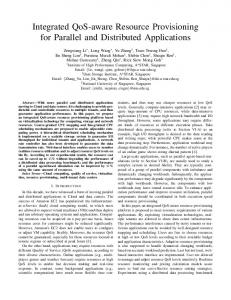
Similarly, we can compute , for all the possible normalized values of the input parameters (i.e., ∈ [0,100], ∈ [0,100]). , is shown in Figure 7. Note The resulting hyper-surface that , ⊆ [−2,2] for any , .
point in time. We use double exponential smoothing [37] because this model has the capability to smooth the inputs and predict the trend in historical data. This model takes the number of requests for application services at runtime and predict the future workload. On the other hand, for estimating response-time, we use single exponential smoothing [37] because for the oscillatory responsetime, we do not need to predict the trend but a smoothed value. Both the exponential smoothing techniques weight the history of the workload data by a series of exponentially decreasing factors. An exponential factor close to one gives a large weight to the first samples and rapidly makes old samples negligible. The specific formula for single exponential smoothing is: =
+ 1−
, > 0;
4.7 The Benefits of Using Type-2 over Type-1 As discussed in Section 4.1, elasticity reasoning is the process of finding a solution for a decision-making problem - choosing an appropriate number of nodes given environmental and system state. As shown in Section 4.6, the output of IT2 FLS is a boundary rather than a hard-threshold as in T1 FLS [29] [35]. Therefore, the decision for nodes can be more flexible providing a boundary. For instance, if the system requires a high performance, the decision can be made based on the upper boundary, i.e. 40,50 = 1.1809 . As a result, two VMs will be added. If the system requires saving cost, the decision can be made based on the lower boundary, i.e. 40,50 = 0.9296 . No new nodes would then be added. In addition, if the system needs to achieve a compromise in user experience and cost, the decision can be made based on any value in the boundary. This flexibility and the ability to handle conflicting rules (see Section 4.6) are the key benefits of T2 FLSs over T1 counterparts that motivated us to choose it for elasticity reasoning.
5. REALIZING THE AUTO-SCALER In Section 4, we described the details of the elasticity reasoning that acts as the heart of RobusT2Scale for making the scaling decisions. In this section, we describe the other modules involves in RobusT2Scale as depicted in Figure 4. First, we describe the prediction module for reasoning input preparations, and then we detail the resource allocator as the actuator of RobusT2Scale. Finally, we describe the details of the integration of these modules.
5.1 Parameter Prediction and Smoothing In historical data corresponding to workload measurements, there are typically high variability, which makes resource allocation at small time-scales unfeasible. As we discussed in Section 2.2 (see challenge 1), the startup time of the VMs are not instant and among the cloud providers, it varies between 60 to 600 seconds [24] but the workload contains many short duration spikes. On the other hand, the elasticity is only effective if node instances can be ready to use when they are needed to serve the workload. Instead of making decisions based on short duration spikes, the elasticity controller needs to identify workload variations that will persist for long enough periods in order to launch or terminate VMs. The term workload refers to a list of user requests and their arrival timestamp. When an application starts running, a time-series forecasting technique is employed to estimate the workload at some future
(5.1)
Correspondingly, the formula for double exponential smoothing is: = + 1− + ) + (1 − ) = ( −
Figure 7. Output of the IT2 FLS for elasticity reasoning.
=
; 0< , ,