Preprint February 14, 2016 – To appear in the Proceedings of the 2016 IEEE International Conference on Robotics and Automation (ICRA 2016)
Autonomous Repositioning and Localization of an In situ Fabricator Timothy Sandy1 , Markus Giftthaler1 , Kathrin D¨orfler2 , Matthias Kohler2 and Jonas Buchli1
Abstract— Despite the prevalent use of robotic technologies in industrial manufacturing, their use on building construction sites is still very limited. This is mainly due to the unstructured nature of construction sites and the fact that the structures built must be larger than the machines which build them. This paper addresses these difficulties by presenting a repositioning and localization system which, using purely on-board sensing, allows a mobile robot to maintain a high degree of endeffector positioning accuracy while moving among numerous building positions during a building task. We introduce a newly developed machine, called the In situ Fabricator (IF), whose goal is to bring digital fabrication to the construction site. The capabilities of the repositioning and localization system is demonstrated through the construction of a vertical stack of bricks, in which the IF repositions itself after placing each brick. With this experiment, we demonstrate that the IF can build with sub-centimeter accuracy over long building sequences.
I. I NTRODUCTION In comparison to other industries, building construction exhibits a surprisingly low level of automation. Off-site prefabrication, in which smaller segments of a building are made at a dedicated factory and then brought to the construction site, is fairly common today [1]. These methods are limited, however, by the constraints that pre-fabricated parts must be transported to the construction site and that it is difficult to adapt these parts to inaccuracies in the building site and the construction process during installation. There has also been significant research in the area of large-scale 3D printing and on-site additive manufacturing [2], [3]. These methods are limited by the fact that the size of the construction machine constrains the size of the building which it can build and that current construction methods and environments cannot be easily adapted to accommodate these processes. For these reasons, our work focuses on developing machines which can build structures directly on construction sites as they exist today. The first conceptual work on using mobile robots for on-site building construction dates back to the 1990s [4]. While more recent projects [5], have demonstrated the ability to build non-standard structures and adapt to inaccuracies within building processes, these processes typically require significant human intervention to reposition and localize the robot. We believe that in order for a robot to effectively build structures at the building scale the machine must be able to 1 Timothy Sandy, Markus Giftthaler and Jonas Buchli are with the Agile & Dexterous Robotics Lab at the Institute of Robotics and Intelligent Systems, ETH Z¨urich, Switzerland. {tsandy, mgiftthaler,
buchlij}@ethz.ch 2 Kathrin Doerfler and Matthias Kohler are with the Chair of Architecture and Digital Fabrication at the Institute of Technology in Architecture, ETH Z¨urich, Switzerland.
[email protected]
Fig. 1.
The IF placing a brick on top of the stack.
move to new building positions and continue building with minimal setup time and effort. In addition, since construction sites are constantly changing environments, reliance on external references and structure within the environment should be minimized. This paper details a system which allows mobile robots to move to requested building positions and reestablish the accuracy needed for construction autonomously and using solely on-board sensing. This work focuses on a newly developed research platform for on-site building construction, the In situ Fabricator (IF). In a previous experiment [6] we constructed an undulated brick wall using the IF in a semi-autonomous manner. The robot was driven manually by remote control and the robot had to be closely supervised to ensure building accuracy. In this paper we present the next step in the IF’s development. Our main contribution is the demonstration that the IF can execute an extended building sequence autonomously and using purely on-board sensing, without exhibiting a degradation in accuracy over subsequent repositioning maneuvers. The remainder of this paper is organized as follows. We first briefly introduce the IF (Sec. II) and the functional structure of its repositioning and localization system. We then discuss the its key functional sub-systems (Sec. III-V). Next we introduce the Brick Stacking Experiment, which was designed to demonstrate the performance of this system (Sec. VI) and present experimental results obtained through tests performed on the IF in a laboratory environment (Sec. VII). The paper concludes with an outlook to future work (Sec. VIII).
BUILDING SEQUENCER
Desired Base Pose
BASE PLANNER
Desired Base Trajectory
BASE STATE ESTIMATOR
BASE TRAJECTORY CONTROLLER
Estimated robot pose
Movement complete
SCANNING & REGISTRATION
ARM PLANNING AND CONTROL True robot pose
Fig. 2.
Repositioning and localization system diagram
II. T HE I N SITU FABRICATOR The IF is a 1.4 ton mobile manipulator with approximately 2.5 m reach which is capable of handling a 40 kg payload. The focus for research on the IF is not to demonstrate that existing building processes can be performed by a robot, but to facilitate the development of new building processes which were previously unachievable using predominantly manual techniques. The IF was designed to be versatile and support a wide range of building tasks. The main functional requirement of the IF is that it can provide 1 mm end-effector positioning accuracy with respect to a global reference frame with no loss in accuracy as the robot moves from one building position to the next. Because construction sites are typically varied and uncontrolled, our goal is to minimize the robot’s dependence on existing structure within its environment. For this reason, the IF was designed to be a completely self-contained machine with fully integrated and on-board control, sensing, and power systems. Importantly, we want to avoid dependence on external reference systems, so that extensive setup and tedious calibration routines are not required. To facilitate its design, building, and maintenance, the IF is composed solely of off-the-shelf components. The IF’s arm is a standard industrial robot arm, an ABB IRB 4600. A retrofitted ABB IRC5 arm controller is mounted on-board. The robot’s base is equipped with hydraulically driven tracks. While the combination of electric and hydraulic power sources is not ideal, this was a design compromise made to reuse existing hardware and minimize robot development time. The system is powered by LI-ion batteries which provide energy for 3-4 hours of autonomous operation. For the experiments performed in this paper, a vacuum gripper is mounted on the arm end-effector. Because this vacuum system is not intended for use on the IF in the long-term it is powered by mains power, which is the only wired connection required for the robot to execute the tasks described herein. The control architecture of the IF’s repositioning and localization system is shown in Figure 2. The Building Sequencer
manages the overall building task, specifying the sequence of building positions and the building tasks which should be performed at each position. It sends a new desired base pose to the Base Planner (described in Section III-A) to initiate a robot repositioning maneuver. Upon successful computation of a collision-free trajectory to the desired position, the Base Trajectory Controller (Section III-C) steers the robot to the desired pose, using pose estimates calculated by the Base State Estimator (Section III-B) in feedback. After completing the base movement, the current estimate of the base pose is used to calculate the expected position of the structure being built (from here on referred to as the workpiece). The Arm Motion Planner and Controller (Section IV) subsequently computes and executes the control actions required to scan an area around the workpiece, using a laser range finder that is mounted on the robot arm end-effector. Point cloud registration (Section V) is then used to localize the robot with respect to the workpiece, returning the resulting robot pose to the building sequencer. Building then continues from that position and the Building Sequencer can request the next base position when appropriate. The components of this control system are discussed in more detail in the following sections. III. BASE NAVIGATION The base navigation sub-system autonomously repositions the IF within the construction site. Once the IF completes the building tasks required in one location (e.g. places a set of bricks), it moves to the next building position, as requested by the building sequencer. Repositioning is performed while avoiding known stationary obstacles in the robot’s workspace. The IF also estimates its position while driving with sufficient accuracy that it can identify and locate where it should continue building once it reaches the desired location. The base navigation sub-system assumes a 2D world. The following section details the trajectory planning, robot pose estimation, and trajectory following control methods used. A. Base Trajectory Planning For robot base trajectory planning, we use STOMP [7], which is a stochastic trajectory optimization algorithm. By generating noisy rollouts, it explores the space around an initial trajectory. The costs of the noisy rollouts are then used to find an updated trajectory with lower cost. The base motion planning is based on a planar, wheeled differential-drive model as given in [8]. Our cost function consists of penalties on the acceleration and jerk of the trajectory as well as non-smooth obstacle costs. The planner assumes a static environment and supports obstacles such as a boundary around the area in which the robot is allowed to move and geometric representations of objects which have already been constructed. Before planning, the movement duration for the whole base maneuver is estimated from the Euclidean distance and orientation difference between initial and final pose and the maximum admissible track velocity.
In order to speed up the convergence of trajectories within STOMP, we found it efficient to run it in two phases. In phase 1, the planner is initialized with an arbitrary trajectory between start and end state, calculated through direct interpolation. Then, we find an initial feasible solution that avoids obstacles but does not respect the robot’s non-holonomic constraints. The second phase uses the solution from phase 1 as initial guess but additionally enforces the non-holonomic constraints of the tracks, which are taken into account as linear constraints for every sample at every time step. The exploration noise is conditioned on the linear constraints as outlined in [9]. B. Base State Estimation Due to the excessive track slip which occurs while a tracked vehicle drives, conventional odometery is not sufficient for tracking the pose of the IF during repositioning. A dedicated state estimator is used instead to estimate the IF’s pose in 2D during repositioning. The robot pose is expressed in reference to the workpiece, with the initial pose set by the result of the previous localization (explained in Section V). Poses are estimated by fusing scans from a laser range finder (Hokuyo UTM-30LX) and gyroscope measurements from an IMU (Xsens MTi-G-700), both mounted rigidly to the base of the robot, in a “pseudo-maximum-likelihood” manner using non-linear least squares optimization with the Ceres Solver [10]. The word “pseudo” is used here because the error function used for scan matching is non-probabilistic. A laser range finder (LRF) is used, as opposed to cameras, because of the low overhead required for scan processing and the potential ability to use the same sensing system to ensure robot workspace safety in the future. Base poses are estimated at the sampling time of the LRF. The latest scan received (referred to as the measurement scan) is fit to a set of earlier scans (called the reference scan) which are spaced over a receding time horizon. Because of the robot’s slow driving speeds, scans are treated as a rigid set of points obtained at the time of the middle point in the scan. Scan matching is performed using an entropybased point cloud quality measure [11]. The error attributed to measurement scan point i is emi =
N X
G(ˆ pM i − pRj , 2σ 2 I),
(1)
j=1
where G(µ, Σ) signifies a Gaussian kernel function centered about µ with variance Σ, pˆM i represents the estimated position of the i-th measurement scan point, given the latest estimate of the robot’s current pose, and pRj represents the j-th reference scan point. Intuitively, this cost function penalizes the pair-wise distances between all points in the measurement and reference scans in a local region whose size is defined by σ 2 . Because measurement and reference scan point pairs have only local influence on the error function, kd-tree-based nearest neighbor searching is used to speed up error function evaluation [12]. Gyroscope measurements are used to improve inference on the robot’s orientation. This is necessary because the scan
matching method used is more sensitive to local minima in the presence of rotational error, as opposed to translational error. Gyroscope measurements are forward integrated to estimated orientation of the robot, θˆk , at the time of a newly received scan. The error attributed to the N gyroscope measurements received between the scans taken at times k−1 and k is N h i X k k k−1 ˆ EG = θ − θ + ωi ∆t . (2) i=1
The robot pose estimated from the M scan points received at time k is "M # X k k TˆW R = argmin emi + cG EG (3) k TW R
i=1
and is found using non-linear least squares optimization. The weighting parameter cG determines the influence of the gyroscope measurements on the estimation result. C. Base Trajectory Controller Once a trajectory is planned to bring the robot to the desired position, a simple P-controller is used find the track velocities (vl and vr ) required to follow the trajectory, using the estimated poses described in the previous section in feedback. The resulting track speeds are set as the reference for the IF’s low-level hydraulic controller. Since driving speed is not a significant concern, we represent the desired trajectory as a time-independent sequence of 2D robot poses, in a similar manner to [8]. The nominal linear and angular velocity of the robot (¯ v k and ω ¯ k , respectively) at each of the poses is also specified in the desired trajectory. When an estimated robot pose is received from the state estimator, the point on the desired trajectory closest to the current pose is found. The nominal linear velocity of that closest point is used directly and the controller computes the angular velocity command. The control law at time k is ωk = ω ¯ k + pt ekt + pθ ekθ ,
(4)
where ekt and ekθ are the translational and angular displacements between the current robot pose and the closest point on the trajectory. The commanded track speeds are then computed from v¯k and ω k . The track speeds are limited for safety. If the one of the track speeds computed exceed these limits as the result of a large ω k , the linear velocity of the robot is decreased. This effectively slows down the robot if it gets far from the desired trajectory, allowing it to turn aggressively and get back on track. The controller gains pt and pθ were tuned to balance trajectory following performance with smooth robot motions. The performance of the base navigation sub-system is discussed Section VII. IV. A RM M OTION P LANNING AND C ONTROL We model the industrial robot arm as a 6-DOF rigid body system with joint state x(t) and joint input torques u(t). The forward dynamics, inverse dynamics and forward kinematics were derived using the Robotics Code Generator [13]. For inverse kinematics we use the Orocos KDL library [14].
For arm motion planning, we replaced the provided path planner of the industrial arm by a custom implementation of iLQG [15] in order to obtain more control over arm motions. iLQG is an iterative nonlinear optimal control algorithm that calculates a time-varying feedforward control as well as time-varying state feedback gains. It iteratively linearizes the system dynamics about the latest estimation of the optimal trajectory and designs LQG controllers for each locally linearized system. We use a cost function of the form tf −1 X J = E h(x(tf )) + l(x(t), u(t)) (5) t=0
where the terminal cost h(x(tf )) penalizes deviations from the desired joint position and velocity. Our intermediate cost l(x(t), u(t)) is dominated by joint velocity and control effort penalties. Before planning, the movement duration is estimated using the assumption that it is proportional to the Euclidean norm of the difference between the initial and desired joint angles. In our case, the algorithm typically converges in less than 5 iterations. Using an efficient, multithreaded C++ implementation [16], locally optimal arm trajectories are generated in less than 2 seconds. Although the planning problem considers control inputs in the form of joint torques, we only send the resulting joint position trajectory to the industrial arm internal controller. The current setup was designed in this way so that it could support the use of dynamic replanning in future work. Note that this planning setup does not include collision avoidance in calculating arm trajectories. Whole sequences of arm motion and object manipulation are created by combining the planned trajectories with a library of pre-programmed manipulation-primitives, such as picking up a brick from the brick feeder, and moving a joint at constant velocity. V. S CANNING AND R EGISTRATION High-accuracy robot localization is achieved by locating the workpiece in point clouds generated using a LRF mounted on the end-effector of the robot arm. After repositioning, the robot scans its environment and the workpiece and ground plane are located in the scan, indicating the robot’s new pose. The following section describes this process in detail. A. LRF Scanning Construction tasks typically afford an abundant amount of prior information about the geometry of a construction site and the workpiece, in the form of a CAD model. For this reason, the scanning strategy chosen for this application matches point cloud measurements directly to geometric representations of the construction site and workpiece. It is assumed that, in the vicinity of the workpiece, the complete geometric form of the construction site is known. In this way, a probabilistic LRF sensor model can be used to find the poses of geometric features in the robot’s environment which maximize the likelihood of acquired point clouds.
Fig. 3.
Point cloud of the brick stack, with the registered brick in red.
The geometry of the construction site and workpiece are represented as a set of parametrically defined geometric primitives (e.g. infinite planes and polygonal faces). Primitives can either represent objects directly (e.g. an infinite plane is used to represent the ground of the construction site), or they can be grouped into a rigid object (e.g. six polygons are grouped to represent one brick). Each object has an associated pose, which is optimized through registration. In the remainder of this section, the notation TROj is used to represent the pose of the object associated with geometric primitive gj in the robot reference frame. Scans are taken when the robot base is stationary. Scan points from the LRF are received in the laser coordinate frame (pL ) and poses, representing the pose of the arm endeffector with respect to its base (TRT ), are received from the arm control system. Linear interpolation is used to find the pose of the arm at the time of each scan point measurement. Combined with the pose of the LRF with respect to the arm end-effector (TT L ), a rigid point cloud of the scan points in the robot frame are built using: pRi = TRT i TT L pLi ,
(6)
where i indicates the i-th scan point. For the remainder of this section, all scan points will be expressed in the robot frame and we will drop the R subscript to simplify notation. To facilitate scanning during sweeping arm motions, laser scan measurements are tightly synchronized in time with the arm pose measurements. This is done by assigning timestamps to the scans and arm poses based on the reception time of digital synchronization pulses transmitted from each device to the robot’s data acquisition system. Digital pulse timestamps are matched with their appropriate data packets by mapping all of the pulse and data packet timestamps to the robot computer’s time frame of reference, using TICSync [17]. While it is difficult to measure the true timing accuracy of the system, we have confirmed that there is no visible discrepancy between points clouds produced by
scanning an object at a distance of 10 m with LRF tilt angular velocities of 3 and 30 ◦ s−1 . B. Object Registration The registration strategy developed for the IF was designed to take advantage of the non-uniform noise characteristics of LRFs. At the distances considered for this application (less than 2 m), LRFs are typically almost an order of magnitude less accurate in the direction parallel to the scan ray than perpendicular to the ray. Specifically, [18] measured that for the UTM-30LX we are using, at a scanning distance of 2 m, the standard deviation of scan points in the direction of the scan ray is 0.018 m, versus 0.0025 m perpendicular to the ray. Registration is formulated as a non-linear least squares optimization problem. An error value is attributed to each scan point, proportional to the distance from that scan point to its nearest geometric primitive, and weighted to account for the non-uniform noise model of the LRF. The first step in computing the error assigned to scan point (pi ) is to find the geometric primitive which is closest to that scan point (g ∗ ), given the current set of estimated object poses. The point on that geometric primitive which is closest to the scan point is then found and the error is calculated as ∗
T
∗
ei = (pi − cp(pi , g )) Σpi (pi − cp(pi , g )),
(7)
where cp(p, g) represents a function which returns the point on geometric primitive g which is closest to scan point p. Σpi represents the covariance of the LRF measurements, rotated such that the direction of highest covariance is parallel to the i-th scan ray. The optimal set of object poses is found by minimizing the sum of squared scan point distance errors. A sufficiently good initial guess for the object poses is required to obtain a good solution. Generally, the initial guess should ensure that each object considered lies close enough to its true location that some of the scan points which actually hit that object when the measurement was taken are identified as being closest to that object. One typical difficulty in dealing with LRF measurements is the presence of so-called “shadow points”. When a scan ray passes closely to the edge of an object, erroneous measurements can be generated in which the returned scan point lies between the object’s edge and the object behind it. We can easily identify when this is the case, however, since we are matching scans directly to the geometry of the scene. When a scan ray lies within some distance of an edge of a geometric primitive, we flag the scan point as a possible shadow point, and if the distance between it and the closest geometric primitive exceeds a threshold, we simply assign zero error to it. Figure 4 shows a point cloud before and after shadow point removal. Table I shows the consistency in registration over a set of 8 scans of a brick in the same position. Four different arm motions were used to create the scans, each consisting of a sweep of a different joint of the robot’s arm. All of the
Fig. 4. Point cloud of a wood block on the ground, before (left) and after (right) shadow point removal. TABLE I C ONSISTENCY IN REGISTERED BRICK POSE FOR 8 SCANS TAKEN USING 4 DIFFERENT SCANNING MOTIONS
x y z roll pitch yaw
Std Deviation 0.44 mm 1.05 mm 0.69 mm 0.056◦ 0.113◦ 0.717◦
scans were taken at the same distance away from the brick to avoid distortion in the scans as discussed in Section VII. C. LRF Extrinsic Calibration The accuracy of the point clouds generated is severely impacted by the accuracy of the relative pose of the laser with respect to the robot’s end-effector in equation 6. The registration package developed for the IF was extended to calibrate this parameter. Although there is not enough space in this paper to fully evaluate our method with respect to existing LRF extrinsic calibration methods, the method used and the results obtained are briefly discussed. Since the scan point pi in Equation 7 is directly related to the extrinsic calibration by Equation 6, we simply need to include the conversion from raw scan points and arm poses to scan points in the robot frame in the error function formulation and we can concurrently solve for the poses of the objects within the scene and the extrinsic calibration. Auto-differentiation is used to avoid the analytic computation of what would be complicated Jacobians. With this method, one can find the extrinsic calibration of the LRF by scanning any object of known geometry. Extrinsic calibration was performed on 9 different datasets. All of the data-sets are made up of a set of 6 to 8 scans taken of a wood cube, of roughly 0.25 m edge length, on top of a flat surface (Figure 4 shows a scan used for calibration). Each scan was generated by sweeping one of the IF’s arm joints in the vicinity of the wood block. The data-sets were acquired with the block in different parts of the robot’s workspace and in a range of lighting conditions. The standard deviation of the calibration values obtained are shown in Table II. The calibration from each data-set was obtained by averaging 20 trials with random initial guesses of the extrinsic calibration and the poses of the ground and wood block in the range of ±0.02 m and 3◦ . The maximum standard deviation of the extrinsic calibration from a single
TABLE II LRF EXTRINSIC CALIBRATION CONSISTENCY OVER 9 DATA - SETS
x y z roll pitch yaw
Fig. 5.
Std Deviation 2.9 mm 1.4 mm 4.1 mm 0.389◦ 0.053◦ 0.389◦
Building sequence for the brick stacking experiment
data-set versus the initial condition was less than 0.5 mm and 0.1◦ , showing good robustness versus initial condition. VI. B RICK S TACKING E XPERIMENT To demonstrate the accuracy and repeatability of the IF’s repositioning and localization system, an experiment was designed in which a vertical stack of bricks is constructed by the robot completely autonomously. After each brick is placed, the robot repositions itself according to a predefined building sequence and place another brick from that location. While this experiment does not produce a structure which is architecturally significant, it was chosen to highlight the mobile autonomy of the robot and provide a clear measure of its building accuracy over numerous repositioning maneuvers. In this task, the IF places a brick and drives in an alternating fashion. The building sequence is defined by a sequence of four building positions, expressed with respect to the stack of bricks. A diagram of the building sequence used is shown in Figure 5. The building positions were chosen to create challenging base repositioning maneuvers (e.g. the robot must change direction two times per loop around the brick stack), and to force the robot to place bricks on the stack from different relative positions. The robot moves between the four building positions sequentially in a loop, creating a repeated hysteresis-shaped pattern around the stack of bricks. VII. E XPERIMENTAL R ESULTS The IF successfully built a 1.3 m high stack of 26 bricks, over the course of a 25 position building sequence. The
average error in brick position was 4.6 mm in the direction of the long face of the bricks and 3.5 mm in the direction of the short face of the bricks. While this error is far from the 1 mm accuracy target set for the robot, the IF did successfully demonstrate its ability to reposition and localize with subcentimeter accuracy and with high repeatability. A video of the brick packing experiment is available online1 . Figure 6 shows the performance of the base navigation sub-system. Shown are the planned and estimated trajectories over the course of four base repositioning maneuvers. At the four positions indicated with arrows, the discontinuous step in estimated robot position shows the update in position resulting from localization with respect to the brick stack. For these repositioning maneuvers, the average error between the desired and estimated (with the Base State Estimator) robot base poses at the end of the repositioning maneuver was 3 cm and 1.8◦ . This shows the accuracy with which the Base Trajectory Controller could lead the robot to the desired position. The average change in base pose after localization was 5 cm and 3.5◦ . This shows how much the Base State Estimator drifted on average during each repositioning maneuver. The resulting base pose after localization was less than 8 cm and 4◦ off from the desired pose originally requested by the Building Sequencer. This shows the accuracy with which the base navigation sub-system as a whole brings the robot to the desired position. These errors were sufficient to allow the robot to re-locate the workpiece with sub-centimeter accuracy in all of the 25 maneuvers executed while building the brick stack. The largest contributing factor to the errors in brick placement seem to come from an unmodeled behavior of the LRF. Up to and during the execution of this experiment almost all of the bricks placed with noticeable positioning error were shifted in the direction from which the scan was taken. This is most likely due to a range measurement bias exhibited by the LRF at short ranges. Figure 7 shows three sets of stationary scans acquired at different heights above the floor of our lab. While the floor isn’t perfectly flat, the bump of about 3 cm height measured by the LRF directly below the scanner is certainly a superficial artifact. The size of the bump increases as the scanner gets closer to the ground, indicating that bias increases at shorter ranges. This behavior was also observed in [18]. It is left as future work to identify and compensation for this behavior. VIII. C ONCLUSION AND O UTLOOK In this paper, we have introduced a repositioning and localization system for the IF. With this system, the IF has demonstrated that it can reposition itself in accordance with a specified building sequence and achieve sub-centimeter object placement accuracy repeatably and over long building sequences. The task was performed completely autonomously and without dependence on external sensing systems or artificial markers placed within the robot’s environment. 1 https://youtu.be/1HPLYOpTYMY
Estimated Position Planned Position
y [m]
1
0
ACKNOWLEDGEMENTS This research was supported by Swiss National Science Foundation through the NCCR Digital Fabrication (NCCR Digital Fabrication Agreement #51NF40 141853) and a Professorship Award to Jonas Buchli (Agreement PP00P2 138920). The authors would like to thank Michael Neunert and Farbod Farshidian for providing their implementation of the iLQG algorithm. R EFERENCES
−1
−2
−1
0 x [m]
1
2
Fig. 6. Planned and estimated robot base trajectories for four repositioning maneuvers. The cross shows the position of the brick stack. The red arrows indicate where the robot stopped and placed a brick.
·10−2 0.4 m height 1.1 m height 2.4 m height
4
y [m]
2
0 −2 −3
−2
−1
0 x [m]
1
2
3
Fig. 7. Stationary LRF scans taken at three heights from the ground. The large bump in the points directly in front of the laser (at x = 0) indicates a bias of the LRF at short ranges.
As a next step, we intend to integrate this system into a large-scale building process and demonstrate it in a more realistic construction site environment. While we have identified one area in which the LRF-based localization system can be improved, we also plan to explore different sensing modalities, such as stereo vision, which will allow for realtime feedback during manipulation tasks. In this way, we hope to get closer to reaching our target of 1 mm accuracy. Beyond the IF sensing system, future work is planned in improving the system’s planning and controls capabilities. In this work, we deliberately avoided motions that would bring the system to the boarders of its dynamic stability limits. Therefore, we particularly intend to push the motion planning and control capabilities beyond the currently used separate arm and base planning, in order to be able to execute dynamic whole-body maneuvers.
[1] U. Knaack, S. Chung-Klatte, and R. Hasselbach, Prefabricated Systems: Principles of Construction. Springer Verlag NY, 2012. [2] B. Khoshnevis, “Automated construction by contour craftingrelated robotics and information technologies,” Automation in construction, vol. 13, no. 1, pp. 5–19, 2004. [3] P. Bosscher, R. L. Williams, L. S. Bryson, and D. Castro-Lacouture, “Cable-suspended robotic contour crafting system,” Automation in Construction, vol. 17, no. 1, pp. 45–55, 2007. [4] J. Andres, T. Bock, and F. Gebhart, “First Results of the Development of the Masonry Robot System ROCCO,” in Proceedings of the 11th ISARC in Brighton (International Symposium on Automation and Robotics in Construction), pp. 87–93, 1994. [5] V. Helm, S. Ercan, F. Gramazio, and M. Kohler, “Mobile robotic fabrication on construction sites: Dimrob,” in Intelligent Robots and Systems, 2012 IEEE/RSJ International Conference on, Oct 2012. [6] K. D¨orfler, T. Sandy, M. Giftthaler, F. Gramazio, M. Kohler, and J. Buchli, “Mobile Robotic Brickwork - Automation of a Discrete Robotic Fabrication Process Using an Autonomous Mobile Robot,” in Robotic Fabrication in Architecture, Art and Design, 2016. [7] M. Kalakrishnan, S. Chitta, E. Theodorou, P. Pastor, and S. Schaal, “Stomp: Stochastic trajectory optimization for motion planning,” in Robotics and Automation (ICRA), 2011 IEEE International Conference on, pp. 4569–4574, May 2011. [8] N. Sarkar, X. Yun, and V. Kumar, “Dynamic path following: a new control algorithm for mobile robots,” in Decision and Control, 1993., Proceedings of the 32nd IEEE Conference on, Dec 1993. [9] M. Kalakrishnan, A. Herzog, L. Righetti, and S. Schaal, “Markov Random Fields for Stochastic Trajectory Optimization and Learning with Constraints,” in Proceedings of Robotics: Science and Systems, 2013. [10] S. Agarwal, K. Mierle, et al., “Ceres solver.” http://ceres-solver.org. [11] M. Sheehan, A. Harrison, and P. Newman, “Self-calibration for a 3d laser,” The International Journal of Robotics Research, 2011. [12] J. Elseberg, S. Magnenat, R. Siegwart, and A. N¨uchter, “Comparison of nearest-neighbor-search strategies and implementations for efficient shape registration,” Journal of Software Engineering for Robotics, 2012. [13] M. Frigerio, J. Buchli, and D. Caldwell, “Code generation of algebraic quantities for robot controllers,” in Intelligent Robots and Systems (IROS), 2012 IEEE/RSJ International Conference on, Oct 2012. [14] R. Smits, “KDL: Kinematics and Dynamics Library.” http://www.orocos.org/kdl. [15] E. Todorov and W. Li, “A generalized iterative LQG method for locally-optimal feedback control of constrained nonlinear stochastic systems,” in Proceedings of American Control Conference, IEEE, 2005. [16] M. Neunert, F. Farshidian, and J. Buchli, “Adaptive Real-time Nonlinear Model Predictive Motion Control,” in IROS 2014 Workshop on Machine Learning in Planning and Control of Robot Motion, 2014. [17] A. Harrison and P. Newman, “Ticsync: Knowing when things happened,” in Robotics and Automation (ICRA), 2011 IEEE International Conference on, pp. 356–363, May 2011. [18] F. Pomerleau, A. Breitenmoser, M. Liu, F. Colas, and R. Siegwart, “Noise characterization of depth sensors for surface inspections,” in Applied Robotics for the Power Industry (CARPI), 2012 2nd International Conference on, pp. 16–21, IEEE, 2012.


![Sensor-based Control and Localization of Autonomous Vehicles in ... [PDF]](https://m.moam.info/img/260x300/sensor-based-control-and-localization-of-autonomou_647d2dd5098a9eb9638b458c.jpg)