Autonomous Virtual Mobile Nodes (Extended Abstract) Shlomi Dolev
Seth Gilbert
Elad Schiller
Dept. of Computer Science Ben-Gurion University
CSAIL, MIT Cambridge, MA 02139, USA
Research Academic Computer Technology Institute
[email protected]
[email protected]
[email protected]
Alex A. Shvartsman
Jennifer Welch
Dept. of Comp. Sci. & Engin. University of Connecticut
Dept. of Computer Science Texas A&M University
[email protected]
[email protected]
ABSTRACT
Keywords
This paper presents a new abstraction for virtual infrastructure in mobile ad hoc networks. An Autonomous Virtual Mobile Node (AVMN) is a robust and reliable entity that is designed to cope with the inherent difficulties caused by processors arriving, leaving, and moving according to their own agendas, as well as with failures and energy limitations. There are many types of applications that may make use of the AVMN infrastructure: tracking, supporting mobile users, or searching for energy sources. The AVMN extends the focal point abstraction in [9] and the virtual mobile node abstraction in [10]. The new abstraction is that of a virtual general-purpose computing entity, an automaton that can make autonomous on-line decisions concerning its own movement. We describe a selfstabilizing implementation of this new abstraction that is resilient to the chaotic behavior of the physical processors and provides automatic recovery from any corrupted state of the system.
mobile networks, ad hoc networks, distributed algorithms, fault-tolerance, location-aware, virtual infrastructure
Categories and Subject Descriptors C.2.1 [Computer-Communication Networks]: Network Architecture and Design—Wireless communication; F.1.1 [Models of Computation]: Models of Computation; D.1.3 [Programming Techniques]: Concurrent Programming— Distributed Programming
General Terms Algorithms,Theory
Permission to make digital or hard copies of all or part of this work for personal or classroom use is granted without fee provided that copies are not made or distributed for profit or commercial advantage and that copies bear this notice and the full citation on the first page. To copy otherwise, to republish, to post on servers or to redistribute to lists, requires prior specific permission and/or a fee. DIALM-POMC’05, September 2, 2005, Cologne, Germany. Copyright 2005 ACM 1-59593-092-2/05/0009 ...$5.00.
1.
INTRODUCTION
Ad hoc infrastructure for mobile ad hoc networks is desperately needed to make these systems usable by applications, allowing developers to overcome the numerous inherent difficulties, such as processors arriving, leaving and moving according to their own agendas, as well as by failures and energy limitations. This paper introduces a new abstraction that extends the focal point abstraction in [9] and the virtual mobile node abstraction in [10]. The new abstraction is that of a virtual general-purpose computing entity, an automaton that can make autonomous on-line decisions concerning its own movement. We call this abstraction an Autonomous Virtual Mobile Node (AVMN). We describe an implementation of this new abstraction that is resilient to the chaotic behavior of the underlying network. Moreover, it guarantees automatic recovery from any corrupted system state. At any given point in time, the AVMN resides at a distinct location. The AVMN is implemented by the processors that happen to be near the AVMN’s current location, thus enhancing the robustness as processors fail and move out of range. The set of processors implementing the AVMN changes over time as the AVMN moves and as the implementing processors move (not necessarily in the same direction). Despite the continually changing set of participants, from a client’s perspective, the AVMN acts like a single, monolithic entity. One of the primary differences between an AVMN, introduced in this paper, and a virtual mobile node (see [10]) is that an AVMN can move autonomously, choosing to move This work is supported in part by the following grants: NSF CCR-0098305, NSF ITR 0121277, NSF 64961-CS, NSF 9988304, NSF 0311368, NSF Career Award 9984774, AFOSR Contract #FA9550-04-1-0121, DARPA Contract #F33615-01-C-1896, and NTT Grant MIT9904-12. The first author and third authors are partially supported by an IBM faculty award, the Israeli ministry of defense, NSF, and the Rita Altura trust chair in computer sciences.
based on its current state and sensor inputs from the physical environment. For instance, if the area to the west of the AVMN appears deserted, then it may decide to move east instead. On the other hand, the AVMN may decide to “hitch a ride” with a subset of the processors currently emulating it. In contrast, the virtual mobile node was required to fix a predetermined path in advance, when the algorithm was deployed, thus significantly limiting the flexibility of the virtual node. Allowing the AVMN to move autonomously introduces several challenges. First, the algorithm must ensure that a consistent set of processors is used to implement the AVMN. When an AVMN decides to move, however, the set of processors participating in the emulation may change; in transitioning from the old set of processors to the new set of processors, the emulator must ensure an orderly transition while maintaining consistency and liveness. The second problem introduced by autonomy is the lack of an a priori location at which the AVMN can be found. Therefore, when the AVMN fails (for example, when it enters an empty region where there are no processors to participate in the emulation), it can be difficult to detect this failure and restore the AVMN. Our AVMN implementation is also self-stabilizing, in that it can tolerate the processors starting from an arbitrary configuration. If a state corruption causes two sets of processors to begin emulating the same AVMN, the emulation algorithm detects this situation and corrects it. Moreover, if the emulating processors become inconsistent (for example, due to network abnormalities), the emulator can recover from the state corruption, and continue to operate correctly.
Roadmap In the rest of this section, we discuss prior work, in particular focusing on virtual infrastructures in wireless ad hoc networks. In Section 2, we present the underlying model for wireless ad hoc networks. In Section 3, we define the required properties of an AVMN in more detail. In the following two sections, we proceed to present a self-stabilizing algorithm to emulate an AVMN. Our implementation consists of two parts. The first part, a basic emulator that operates correctly once a consistent set of participants has been determined, is presented in Section 4. The second part ensures that the set of participants eventually stabilizes to a consistent set, and is presented in Section 5. We present some discussion and optimizations in Section 6.
Previous work In [9], we presented a new approach, called GeoQuorums, for implementing atomic read/write shared registers in mobile ad hoc networks. This approach is based on associating abstract atomic objects with certain geographic locations called “focal points”. These geographic locations are assumed to be normally populated by mobile processors. In [10], we generalized our approach from [9] from stationary atomic objects to mobile virtual nodes. We assumed that the virtual nodes moved on a fixed trajectory that was globally known in advance. We presented a new replicated state machine algorithm to implement the virtual node using a constantly changing set of processors in the vicinity of the virtual node’s current location. In contrast with [10], our current work relaxes the assumption that the trajectory of each virtual entity is fixed and
known in advance. Furthermore, the new abstraction is selfstabilizing and automatically regenerating. Fixed-location self-stabilizing virtual stationary automata for different settings appear in [8, 11]. As discussed above, the introduction of autonomy introduces several new difficulties. The idea of executing algorithms on virtual mobile entities was inspired by compulsory protocols [6, 14, 19], which assume that some subset of the processors can control their own motion. They showed that this assumption significantly simplifies the design of protocols, compared to an environment in which processors move in an unpredictable or adversarial manner. The work in [10] on virtual mobile nodes generalizes Beal’s Persistent Node abstraction [1, 2], in which nodes travel in a static network carrying limited state. The work of Nath and Niculescu [22], in which messages are routed along a particular trajectory, and Geocast (e.g., [5, 17, 23]), in which data is routed geographically, are connected to this work in that they can be seen as attempts to simulate a traveling processor with limited functionality.
2.
BASIC SYSTEM MODEL
The system consists of a set of communicating mobile entities, which we call processors. We denote the set of processors by P, where |P| = n ≤ N ; N is an upper bound on the number of processors, and is known by the processors themselves. In addition we assume that every processor has a unique identifier. The processors communicate among themselves using a local broadcast primitive, with radius Rlb . The local broadcast is assumed to be reliable, meaning that every processor that stays within distance Rlb of the sending processor is guaranteed to receive the message exactly once, and to deliver the message within d time of its being sent. This is an abstraction of some Ethernet-like service. The operations are denoted LBcast and LBrecv. There is a Geocast service, by which a processor can send a message to all processors in some specified geographic area. We also assume the Geocast is reliable and that there is an upper bound D ≫ d on the latency of Geocast messages. A number of Geocast routing protocols have been proposed for mobile ad hoc networks (see [25] for a survey and comparison). The operations are denoted Geocast and Georecv. Finally, we assume that there is a reliable time and location service available to each processor, such as would be provided by GPS. The existence of a reliable time and location service makes it easy to implement the local broadcast and Geocast communication services in a self-stabilizing way, by differentiating current messages from previous (possibly corrupted) messages. Several processes can run in a single processor. The inputs to a process include the receipt of a message destined for itself, either from another processor or from the same processor. For instance, there could be a process associated with a sensor on the processor that sends data to another process on the same processor. Every processor pi executes a program that is a sequence of steps. For ease of description, we assume the interleaving model where steps are executed atomically, a single step at any given time. Each step of pi is triggered by an input, which is either the receipt of a message or a timer going off. The state si of a processor pi consists of the value of all the variables of the processor including the value of its program counter. The execution of a step in the algorithm can change the state of a processor.
We let the undirected graph G(V, E) denote the current communication graph of the system, where V is the set of processors, together with their coordinates in the plane, and there is an edge in E between processors pi and pj if and only if the two processors can communicate with each other using the local broadcast service. (This depends on whether the two processors are within Rlb of each other). Notice that G changes over time. The term system configuration is used for a tuple of the form (s1 , s2 , · · · , sn , G(V, E)), where each si is the state of processor pi (including messages in transit for pi )and G(V, E) is the current communication topology. Therefore the vector of individual processor states and the current communication graph fully describes the system state. We define an execution E = c0 , st0 , c1 , st1 , . . . as an alternating sequence of system configurations ci and steps sti , such that each configuration ci+1 (except the initial configuration c0 ) is obtained from the preceding configuration ci by the execution of the step sti . In addition, sti may reflect a change in the communication graph. Thus, the only components that can be changed due to the execution of sti are the state of p, the state of a neighbor of p and the communication graph G(V, E). An execution is fair if every processor executes a step infinitely often. An external trace of an execution is the subset of execution steps consisting of Geocast and Georecv events. In some of our algorithms, random walks are used for broadcasting information. We consider the subset of fair executions in which a message sent in a random walk fashion succeeds in arriving at all processors in the system in a timely fashion. In more detail, a nice execution [12] is defined to be an execution in which a message sent in a random walk fashion arrives at every processor after no more than M consecutive message send operations, where M is a function that depends on n. The probability of having a nice execution in several common cases is computed in [12] using techniques from random walks. The probability is calculated assuming an arbitrary initial configuration and relies on known results about the cover time of random walks in graphs. (See, for example, [20] for standard calculations of cover times in various graphs). For our algorithms that use random walks, we prove that in every nice execution our algorithms are correct. In this way we abstract away the probabilistic analysis, which allows us to present and analyze our algorithms in a deterministic framework.
3. AUTONOMOUS VMNS An Autonomous Virtual Mobile Node (AVMN) is an arbitrary automaton that resides, at any given time, at a specific location in the network; it can communicate with nearby processors, using the local broadcast service (LBcast), and can send and receive Geocast messages in the same way as a real processor residing at its location. The AVMN is specified in terms of (1) a set of states, V , (2) an initial state, v0 , (3) a set of inputs, inputs, (4) a set of outputs, outputs, and (5) a transition function, δ, mapping from states and inputs to states and outputs. An algorithm implementing an AVMN must satisfy the following property: Property 1 (Correct emulation of the AVMN). For every execution of the emulator, there exists an execution hc0 , st0 , c1 , st1 , . . .i of the AVMN automaton such that the external traces are equivalent.
Unlike a (mobile) processor, an AVMN controls its own motion: an AVMN moves in discrete steps from one location to another. An AVMN specification, then, also includes a movement function, calculate-location, which determines a new location for the AVMN as a function of its current location, current time, and current state. Finally, an AVMN is robust. As long as there are real processors near the AVMN, it remains alive. There are two ways an AVMN can fail: either it enters an empty region of the network, or it suffers a state corruption, potentially causing multiple copies of the AVMN to appear in the network. (A state corruption may occur when some network assumption, such as reliable wireless communication, is temporarily violated.) In either case, the AVMN can recover. Property 2 (Exactly one AVMN). For every execution of the emulator, in every configuration, there is exactly one copy of an AVMN in the network. An AVMN emulator is self-stabilizing when in every fair execution (respectively, nice execution, for algorithms that depend on random walks), starting from an arbitrary configuration there is a suffix in which Properties 1 and 2 are satisfied. The program (including the AVMN code) of the processors is assumed to be (hardwired and) correct, namely, we do not assume Byzantine behavior of the processors. Note that an AVMN-simulation process needs to be running all the time, even if just listening to messages to see if it should start participating. We also assume that the program has information concerning N , the upper bound on the number of processors and the identifier of the processor. We remark that an application that uses an AVMN as a computing platform should be self-stabilizing as well, since the AVMN may start correct execution of the application itself in an arbitrary state.
4.
AVMN IMPLEMENTATION
In this section we describe the basic algorithm to emulate an AVMN, assuming all the participants in the emulation are near, within some fixed Ravmn < Rlb of, the unique location of the AVMN, that is, assuming the AVMN has a consistent set of participants. In Section 5, we show how to ensure that there is a consistent set of participants. The pseudocode for the basic AVMN emulator appears in Figure 1 (and all line numbers refer to this figure).
Replication Each participating processor keeps a replica of the AVMN’s current state and a buffer of input events waiting to be applied to the state. It is sufficient to keep only the events that have occurred within the last 2d time units, where d is an upper bound on the latency of the local broadcast service (see lines 42–43). The emulation protocol must ensure that state transitions of the AVMN are atomic and identical in all replicas. A state transition can be triggered by inputs, such as the messages arriving (via Geocast) at a participating processor, sensor inputs, or the clock reaching a certain value. When a processor receives a Geocast message, it broadcasts a georecv message using the LBcast service indicating that an event occurred (line 34). Similarly, when a processors detects a sensor input, it broadcasts a sensor message (37). When a
Variables: 1 2 3 4 5 6
status, in {idle, joining, active} state, state of the replica location, current AVMN location buffer, buffer for incoming messages last−refresh, last time a state refresh occurred clock, real time clock
Externally specified functions/constants: 8 9 10 11 12 13 14
v0 , the initial state of the AVMN δ, the AVMN transition function calculate−location(. . .), calculates the next location of the AVMN recover(. . .), deterministically chooses a new state tmove , frequency of AVMN movement tref resh , frequency at which state is refreshed tprocess , frequency at which AVMN takes spontaneous steps
Transition functions: 16 17 18 19 20 21 22 23 24
init(ℓ ) location ← ℓ state ← v0 buffer ← ∅ last−refresh ← clock status ← active settimer(next−multiple(tprocess , clock), Process) settimer(next−multiple(tref resh , clock), Refresh) settimer(next−multiple(tmove , clock), Move)
27 28 29 30 31
LBrecv(m) if (m = hnew−loc, ℓ i) and (status = idle) then location ← ℓ else buffer ← buffer ∪ hm, clocki settimer(clock+d, NewMessage)
34
Georecv(m) LBcast(hgeorecv, m)i)
37
onSensor(s) LBcast(hsensor, si)
39 40 41 42 43 44
onTimer(Process) if ∃ x : δ(state, Geocast(x)) 6= ⊥ then LBcast(geocast, x) ∀hm, ti ∈ buffer : t < clock−2d do buffer ← buffer \ hm, ti settimer(next−multiple(tprocess , clock), Process)
47 48
onTimer(Move) LBcast(move, location, clock) settimer(next−multiple(tmove , clock), Move)
51 52 53 54 55 56 57
69 70 71 72 73 74
76 77
79 80
82 83 84 85 86 87
89 90 91 92
49 50
66 67
88
45 46
64 65
81
38
onNewLocaction(ℓ ) if (|ℓ −location|) < R then if (status = idle) then status ← joining last−refresh ← clock cleartimers() else status ← idle
onTimer(Refresh) LBcast(hstate, state, buffer, clocki) last−refresh ← clock settimer(next−multiple(tref resh , clock), Refresh)
63
78
35 36
61 62
75
32 33
60
68
25 26
59
93 94 95 96 97 98 99
onTimer(NewMessage) let m = min(m : hm, ti ∈ buffer, t = clock−d) if (m = hnew−loc, ℓ i) then location ← ℓ if (status = active) then if m = hsensor, xi then states ← δ(state, onSensor(m)) else if m = hgeorecv, xi then states ← δ(state, Georecv(m)) else if m = hgeocast, xi then states ← δ(state, Geocast(m)) Geocast(x) else if m = hmove, loc, move−timei then if (loc = location) then location ← calculate−location(location, clock, state) LBcast(new−loc, ℓ ) else if m = hstate, x, y, lri then let S = {m : m = hstate, w, z, lri} if (|S| > 1) or (status = joining) then state ← recover(S) if (|S| = 1) then buffer ← ∅ else if (status = joining) then let J = {hm, ti ∈ buffer : lr−d < t ≤ clock−d} while J 6= ∅ let m′ = min(J) if m = hsensor, xi then states ← δ(state, onSensor(m)) else if m = hgeorecv, xi then states ← δ(state, Georecv(m)) else if m = hgeocast, xi then states ← δ(state, Geocast(m)) J ← J \ m′ buffer ← buffer \ m′ status ← active settimer(next−multiple(tref resh , clock), Refresh)
Figure 1: The AVMN emulation algorithm. When the emulator is started, the init function is called, which initializes three timers: a Process timer that allows the emulator to take steps, a Refresh timer that performs consistency checks, and a Move timer that causes the AVMN to move. From that point onwards, the emulator is driven by timer interupts, message interupts, and sensor interupts: when a timer expires, the appropriate onTimer function is invoked; when a message is received, either LBrecv or Georecv is invoked; when a sensor produces a reading, onSensor is invoked.
processor decides to send a Geocast message (lines 39–44), it broadcasts a geocast message. On receiving a message (lines 26–31), an additional delay of d (the maximum broadcast delay) is imposed (via a timer—line 31) to ensure that all processors process the events in the same order. This ensures that the state is updated consistently at all replicas. To ensure that the replica states remain identical among all the processors that emulate the AVMN, in spite of faults and corruptions, each processor, at a fixed interval, trefresh , sends its replica state and message buffer (or a hash function thereof) to all the other emulating processors (lines 59–62). Upon receiving all the messages, each processor waits until at least d time has elapsed since the checkpoint messages were sent (by examining the timestamps). Then, if there are any conflicts, that is, the checkpoints received are not identical (line 82), a predetermined recovery function is applied (line 83), and the buffers are flushed (lines 84–85).
Joining When a processor enters the “sphere of influence” of an AVMN, that is, within Ravmn , it should start participating in the simulation of the AVMN (lines 50–57). The joining processor sets is status to joining, and waits for a state refresh. During this time, it listens, saving the events in its buffer. After d time passes, it has the same buffer as all other actively participating processors. Therefore, the first time the processor receives a state refresh that was initiated at least d time after it began listening, it can complete the join protocol by adopting the new state (lines 86–99). (Note that in an optimized version where only a hash is sent, the joining processor will have to request the state explicitly.) Suppose, as in Figure 2, the joiner starts the join procedure at time t (setting its own last − refresh to t). The joiner takes the first replica state that it receives with timestamp (i.e., the lr component of the message) at least t + d. Call this timestamp t′ . The joiner collects all the replica states with timestamp t′ , checking for consistency. The joiner then adopts this state and replays all messages that it has received with timestamp greater than last−refresh−d using the usual delivery algorithm, processing the messages in order of their timestamp, ignoring message sent in the last d time and breaking ties in some consistent way.
Navigation A key feature of the AVMN abstraction is that it can decide autonomously where to move. The decision is a function of the current state of the AVMN, which may encode information concerning the current environment. With a fixed frequency, tmove , a processor participating in the emulation initiates movement by broadcasting a move message using the LBcast service (lines 46–48). Notice that this broadcast message does not actually specify the location, as might be expected. In fact, each processor independently calculates the new location, based on the old location, the time of the move, and the current state (line 78). The primary purpose of this broadcast message is to order the movement with respect to the other messages and events being processed, in order to ensure that the move occurs consistently at all processors. As a result, when the new location is calculated, all the processors have the same replicated state, and therefore choose the same new location. After the new location is calculated, a new-loc message
is broadcast notifying all the processors of the new AVMN location (line 79). Only participating processors can calculate the new location themselves; other processors that are not participating receive the new-loc message, updating themselves on the current location. Without this additional message, no new nodes would be aware of the new location and would be unable to join the emulation. In order that enough old nodes remain participants, and that enough nodes near the new location can receive the notification, we impose an additional limitation on the speed of motion. Let ǫ be the maximum distance moved by the AVMN in a single transition. Then we assume that Rlb ≥ 2 · Ravmn + ǫ. Theorem 3. Consider an execution E of the AVMN emulator. Assume that there is a suffix of the execution, E ′ = ci , sti , ci+1 , sti+1 , . . ., such that in configuration ci there is a consistent set of participants. Then there exists some j ≥ i and an execution E ′′ of the AVMN automaton such that the external trace of E ′′ is equal to the external trace of the suffix of E ′ beginning with configuration cj . Proof sketch. First, notice that after some period of time all messages sent prior to ci in execution E have been delivered and then removed from the processor’s buffers (in line 43). Moreover, notice that time d after the next RefreshState, each processor examines the state messages sent when the Refresh timer expired (lines 80 − −99). If all the active processors sent the same checkpoint (i.e., |S| = 1), then we let cj be the configuration when the Refresh timer expired. Otherwise, we let cj be the configuration immediately after each processor has completed the recovery (lines 83–85). In either case, every processor has the same state and buffer in configuration cj ; we therefore choose the state component of one of the processors in configuration cj as the initial state in execution E ′′ . It remains to show that the participants continue to consistently update their replicated state; since all the processors update their state according to δ, we can use the sequence of updates to devise the rest of execution E ′′ . Notice that every participating processor that is within distance Ravmn of the AVMN location processes messages in the same order. Before processing a message, m, a processor delays d time, therefore by the time m is removed from the buffer, every message sent prior to m has been received. Therefore, there exists a total ordering of all messages, based on the time they were sent; every processor removes them from the buffer in that order. The proof then follows by induction on the sequence of messages processed. The following two invariants are maintained: (1) all processors have the same replica state after processing message mk , (2) the set of participating processors is consistent. This follows by a case analysis of the messages processed. If mk is a simulation message, that is, sensor, geocast, or georecv, then the state is consistently updated at all processors by applying m to the current state, which by induction and consistent message ordering is the same at all nodes. If mk is a state message, then either the states are already consistent, or recovery begins. In the case of recovery, the buffers are cleared and the state is set to a deterministically calculated value. In the case of joining, a new processor has acquired the same buffer as each of the current participants by listening to the messages for an interval of at least time d, and thus the state is updated
mj mj
active
hstate, t′ i joiner time
t
mi mj t − d t′ t′ + d ′
t′ ≥ t + d Figure 2: The joiner adopts state received at time t′ + d, quickly replays the mi , mj messages, and then is caught up. Note that in the figure, the mi , mj messages are sent in the interval [t′ − d, t′ ] and delivered in [t′ , t′ + d]. consistently, resulting in a successful join. If mk is a move message, then each processor that receives the message is either still near the new center, in which case it remains a participant, or it is far from the new center, in which case it leaves; the set of participants remains consistent. If mk is a new-loc message and pi is not active, it simply adopts the new location; since it was previously not a participant, the set of participants is still consistent. If pi is active, then it already has updated its location. Since the replicated state of the emulator is updated consistently, we can apply the same updates to execution E ′′ , generating an execution of the AVMN automaton. Since Geocast messages are only generated by a processor when such a broadcast is a legal step of the AVMN, it is clear that the external trace of the emulator—after configuration cj —is equal to the external trace of E ′′ .
5. ENSURING EXACTLY ONE AVMN Recall that Theorem 3 guarantees a consistent execution from that point at which there is a consistent set of participants. In this section, we describe how to stabilize on a consistent set of processors to emulate the AVMN, presenting three schemes for ensuring the existence of exactly one instance of an AVMN.
Virtual Stationary Automata Scheme The first scheme uses a virtual stationary automaton (VSA) to keep track of the AVMN. A VSA is another type of virtual infrastructure component, introduced in [11]. Unlike an AVMN, it is stationary, fixed in a single predetermined location. Much like an AVMN, it is emulated by a set of continually changing participants. Since it is stationary, however, the issues of autonomy do not arise. In particular, for a VSA it is trivial to ensure a consistent set of participants: they are exactly the set of participants that are near the VSA’s fixed location. One could therefore implement a VSA using the algorithm in Section 3, instead of the algorithm in [11]. A VSA, if available, can be used to simplify the problem of maintaining a consistent set of participants in an AVMN. The AVMN uses a Geocast service to send “I am alive” messages to the region containing the VSA. If the VSA does not receive an “I am alive” message for too long a period, the VSA creates a new AVMN. The VSA is also responsible for the elimination of undesired copies of an AVMN. Each “I am alive” message carries the location of the AVMN and
the timestamp at which the message was sent. The VSA can easily detect that more than one copy of the AVMN exists and send an elimination message to all but one of them. The scheme can be naturally extended to a more fault tolerant, distributed version in which several VSAs are responsible for the existence of the AVMN, each having a different time-out period to avoid simultaneous creation of multiple copies. Lemma 4. Starting from an arbitrary initial state, the VSA Scheme ensures a consistent set of participants in any nice execution. Proof sketch. If there is no AVMN in the network, then eventually the VSA stops receiving “I am alive” messages and creates a unique new one. If there is more than one AVMN in the network, then eventually the VSA eliminates all but one. We note that, in the VSA Scheme, starting from an arbitrary configuration, we reach a consistent set of participants within: (1) the time it take the VSA to stabilize, plus (2) the Geocast time.
Token Random Walk Scheme In the second scheme, the mobile processors themselves verify the existence of the AVMN, without relying on an auxiliary VSA. The AVMN repeatedly sends out a token containing the message “I am alive.” The token travels on a random walk through the ad hoc network, until its timeto-live expires. If a processor does not receive an “I am alive” token for, say twice, the expected random walk cover time (see [12, 20], for example, for cover time bounds), then it generates a token containing a “formation” message and the processor’s identifier and a time-to-live that bounds the token’s lifetime. The formation token itself travels on a random walk. When two formation tokens collide, they merge, maintaining a collection of processor identifiers. When a formation token contains ⌈(N + 1)/2⌉ processor identifiers, the (single) processor that holds the token creates a new AVMN. To ensure that there is eventually only one copy of the AVMN, each AVMN monitors the “I am alive” messages in the network, each of which includes a timestamp and a location. The AVMN, which maintains a bounded location history, can thus determine if a token belongs to a duplicate AVMN, and determine using a deterministic function whether to eliminate itself. Only a bounded history is
needed since there exist bounds on how long it takes a token to cover the network in nice executions. Lemma 5. Starting from an arbitrary initial state, the Token Random Walk Scheme ensures a consistent set of participants. Proof sketch. If there is no AVMN in the system, eventually each processor produces a formation token. Eventually, the formation tokens collide, forming a unique AVMN. If there is more than one AVMN, eventually each AVMN receives “I am alive” tokens from the other AVMNs. All but one AVMN will then be eliminated. We note that, in the Token Random Walk Scheme, starting from an arbitrary configuration, we reach a consistent set of participants within O(M ) time, where M is the time it takes for a random walk to visit every node.
Stay Alive Scheme The third scheme is different in the sense that the AVMN itself does not send messages. Instead, processors at predefined times (say every hour on the hour) send tokens containing a “stay alive” message on a random walk of the network. Eventually the AVMN should receive the tokens. In every time period the AVMN must collect at least ⌈(N + 1)/2⌉ stay alive tokens in order to survive to the next time period. Notice that if there is more than one copy of the AVMN, at most one is able to collect a majority of stay alive tokens in a time period. If a stay alive token survives for too long without finding an AVMN, it begins to act like a formation token in the Token Random Walk scheme: when two stay alive formation tokens collide, they merge, and when a majority of stay alive formation tokens have merged, they form a new AVMN. Lemma 6. Starting from an arbitrary initial state, the Stay Alive Scheme ensures a consistent set of participants in any nice execution. Proof sketch. If there is no AVMN in the system, eventually the tokens all become formation tokens, and eventually all merge and form a new AVMN. If there is more than on AVMN in the system, at most one is able to collect a majority of the tokens, and therefore at most one AVMN survives. As in the Token Random Walk Scheme, in the Stay Alive Scheme, when starting from an arbitrary configuration, we reach a consistent set of participants within O(M ) time, where M is the time for a random walk to visit every processor.
stable state when there exists one AVMN, there only needs to be a small number of tokens performing random walks in the network. It is only in the case of formation that all the processors need to create tokens. The Stay Alive scheme is the least efficient, in terms of messages. All the processors need to create tokens at all times. However, it is simpler than the Token Random Walk scheme, in that only one type of token is needed. Moreover, the AVMN does not have to send any heartbeat messages. Using any of the three schemes, we can combine Lemmas 4–6 with Theorem 3 to conclude our main theorem: Theorem 7. The AVMN emulator, using any of the three schemes, is a self-stabilizing implementation of an arbitrary automaton.
6.
DISCUSSION
We have discussed in this paper how to implement a single AVMN; one could instead implement multiple AVMNs using the same techniques. It is possible to create the AVMNs dynamically, allowing them to collaborate to perform differing tasks. Moreover, AVMNs might be organized into a hierarchy, improving efficiency for tasks such as tracking and communication. There are a number of ways to optimize the movement of the AVMN so as to minimize the energy needed. First, the processor can use the minimum amount of power necessary to reach everyone at the current AVMN location. Second, we can use the mobile processors that are closer to the new AVMN location to perform the broadcast, thus requiring less energy to reach everyone. Third, if the AVMN motion is dependent on the mobile processor’s motion (for example, in the case of tracking), then we can take advantage of the movement to minimize the energy needed. The algorithm presented can be optimized in many ways, for example, the communication overhead can be significantly reduced by using checksums (instead of sending the entire state) and/or using randomization to limit the number of processors broadcasting consistency-check messages. When an inconsistency is detected, we can use an ethernetlike algorithm to choose randomly which replica will survive (it will be the first that succeeds in performing local broadcast). We also note that there are ways to change the AVMN program that is assumed to be hardwired in each processor. One way to do so is by using a super-user message that is sent to all the processors (say, with the assistance of VSAs) to replace their code. Our approach can also be generalized to work in three dimensions, rather than two — instead of a disc around the AVMNs location, we may consider a ball.
Trade-Offs The VSA scheme is the most efficient, in terms of messages required. Unlike the other two schemes, messages can be sent directly to a known location, rather than performing a random walk of the network. For the same reason, the VSA scheme is able to respond most rapidly to abnormalities in the system. In fact, the simplicity of this scheme is yet another example of the utility of having virtual, reliable infrastructure in a mobile ad hoc network. On the other hand, the VSA scheme requires maintaining a stationary virtual automaton. The Token Random Walk scheme is also relatively message efficient, in that in the
7.
REFERENCES
[1] J. Beal, “Persistent nodes for reliable memory in geographically local networks,” TR AIM-2003-11, MIT, 2003. [2] J. Beal, “A robust amorphous hierarchy from persistent nodes,” Proc. of Communication Systems and Networks, 2003. [3] O. B. Bayazit, J.-M. Lien, and N. M. Amato, “Roadmap-Based Flocking for Complex Environments,” Proc. 10th Pacific Conference on Computer Graphics and Applications (PG’02), 2002.
a
b
Rlb
Rlb
q p
q p
X
X Ravmn
X’ Ravmn
Figure 3: a) Processor p participates in an AVMN at location X and informs processor q about relocation to X ′ using an Rlb broadcast. b) Processor q participates in an AVMN at new location X ′ that is ǫ distance units away. [4] J. Bohn and F. Mattern, “Super-Distributed RFID Tag Infrastructers,” TR, Institute of Pervasive Computing, ETH, 2004. [5] T. Camp and Y. Liu, “An adaptive mesh-based protocol for geocast routing,” Journal of Parallel and Distributed Computing: Special Issue on Mobile Ad-hoc Networking and Computing, pp. 196–213, 2002. [6] I. Chatzigiannakis, S. Nikoletseas, and P. Spirakis, “An efficient communication strategy for ad-hoc mobile networks,” Proc. 15th International Symposium on Distributed Computing, 2001. [7] P. Chandler and M. Pachter, “Hierarchical Control for Autonomous Teams”, AIAA Guidance, Navigation, and Control Conference and Exhibit, 2001. [8] S. Dolev and O. Gersten, “Robust Active Super Tier Systems”, Proc. of the IEEE International Conference on Software-Science, Technology and & Engineering, 2005. [9] S. Dolev, S. Gilbert, N. Lynch, A. Shvartsman, and J. L. Welch, “GeoQuorums: Implementing Atomic Memory in Ad Hoc Networks”, Proc. 17th International Symposium on Distributed Computing (DISC), pp. 306–320, 2003. To appear in Distributed Computing. [10] S. Dolev, S. Gilbert, N. Lynch, E. Schiller, A. Shvartsman, and J. L. Welch, “Virtual Mobile Nodes for Mobile Ad Hoc Networks,” Proc. 18th International Symposium on Distributed Computing (DISC), pp. 230–244, 2004. [11] S. Dolev, S. Gilbert, L. Lahiani, N. Lynch, and T. Nolte, “Virtual Stationary Automata for Mobile Networks”, TR MIT-LCS-TR-979, MIT CSAIL, Cambridge, MA 02139, January 2005. [12] S. Dolev, E. Schiller, and J. L. Welch, “Random Walk for Self-Stabilizing Group Communication in Ad-Hoc Networks,” Proc. 21st Symp. on Reliable Distributed Systems, pp. 70–79, 2002. To appear in IEEE Transactions on Mobile Computing. [13] D. Gillen and D. Jaques, “Cooperative Behavior Schemes for Improving the Effectiveness of Autonomous Wide Area Search Munitions”, Proceedings of the Cooperative Control Workshop, 2000.
[14] K. P. Hatzis, G. P. Pentaris, P. G. Spirakis, V. T. Tampakas, and R. B. Tan, “Fundamental control algorithms in mobile networks,” Proc. of the 11th ACM Symposium on Parallel Algorithms and Architectures archive, Saint Malo, France, 1999. [15] J. Hebert, “Cooperative Control of UAVs”, AIAA Guidance, Navigation, and Control Conference and Exhibit, 2001. [16] E. Kivelevich and P. Gurfil “UAV Flock Taxonomy and Mission Execution Performance”, Proc. of the 45th Israeli Conference on Aerospace Sciences, 2005. [17] F. Kuhn, R. Wattenhofer, Y. Zhang, and A. Zollinger., “Geometric Ad-Hoc Routing: Of Theory and Practice”, Proc. of the 22nd Symp. on the Principles of Distributed Computing, July 2003. [18] L. Lamport, “Time, clocks, and the ordering of events in a distributed system,” Communications of the ACM, 21(7):558–565, 1978. [19] Q. Li and D. Rus, “Sending messages to mobile users in disconnected ad-hoc wireless networks,” Proc. 6th MobiCom, 2000. [20] R. Motwani and P.Raghavan, “Randomized Algorithms.” Cambridge University Press, 1995. [21] R. Nagpal, H. Shrobe, and J. Bachrach, “Organizing a global coordinate system from local information on an ad hoc sensor network,” 2nd Workshop on Information Processing in Sensor Networks, 2003. [22] B. Nath and D. Niculescu, “Routing on a curve,” ACM SIGCOMM Computer Communication Review, 33(1):150 – 160, 2003. [23] J. C. Navas and T. Imielinski. “Geocast – geographic addressing and routing,” Proc. of the 3rd MobiCom, 1997. [24] N. B. Priyantha, A. Chakraborty, H. Balakrishnan. “The cricket location-support system,” Proc. 6th ACM MOBICOM, 2000. [25] P. Yao, E. Krohne, and T. Camp, “Performance Comparison of Geocast Routing Protocols for a MANET,” Proc. of the 13th IEEE International Conference on Computer Communications and Networks (IC3N), pp. 213–220, 2004.