can operate as a mobile reference point equipped with ultra sound transmitters. ..... and the dispatch of the signals within the whole hemisphere. However ..... environment,â in IEEE Workshop on Software Technologies for Future. Embedded ...
Self-localization Capable Mobile Sensor Nodes Juergen Eckert, Kemal Koeker, Philipp Caliebe, Falko Dressler and Reinhard German Computer Networks and Communication Systems Department of Computer Science, University of Erlangen, Germany {juergen.eckert, koeker, philipp.caliebe, dressler, german}@informatik.uni-erlangen.de
Abstract—Position sensing systems for indoor environments have one common problem: The setup effort of the whole system. GPS-supported localization is simple and fast to implement and the reference grid is ubiquitous. However, in locations where the signals of GPS are not available, e.g. indoor, or where the technique is not accurate enough, other position sensing systems have to be used. Usually, a reference grid will be provided by an administrator: Reference points must be deployed and programmed with the correct location information. Especially for temporary installations and dynamic surroundings the setup costs are very high. In our work, we developed a robotic platform, which is capable of deploying itself autonomously and which can operate as a mobile reference point equipped with ultra sound transmitters. Relying on a combination of two controllers and an odometry system, the platform is able to drive on a complex spline-like trace using only a few supporting points. We also investigated the problem for the localization system itself. The detection field of our ultra sound based system is a full hemisphere. Within this domain, we can measure the distances between nodes exploiting the time of flight technique as well as the angle of arrival. Finally, the system can also be used as a sonar system for passive obstacles detection. Index Terms—Indoor localization, sensor network, ultrasound, autonomous robot
I. I NTRODUCTION Sensor network applications can benefit in many ways from the knowledge of their current physical position. For outdoor scenarios, this can be accomplished in an easy and fast manner by using the global positioning system (GPS). However, for indoor scenarios positioning has to be based on other methods. In general, two different techniques are possible. First, a device can enter an unprepared environment and localize itself relying on (passive) observations and an a priori provided map [1]. Secondly, a device can localize itself by relying on interactions with other devices – which is similar to GPS. We focus on the latter solution to enable the operation in unknown environments. Although a considerable amount of academic or commercial systems are available, there is no widely accepted approach available so far. Based on the complexity of the various scenarios, the available systems are normally designed for a specific application and not applicable for general usage. In most cases, the biggest hurdle limiting the wide propagation of the various localization systems is the preparation of the localization grid itself. As a persistent localization system is usually not desired, the grid assembly and disassembly effort is not negligible. For example, the GPS grid is maintained by the US government and is available worldwide. Each GPS client can determine its position referring to this grid
Fig. 1.
Mobile sensor node including localization hardware
without any additional administrative effort. However, for indoor position sensing this is, of course, not easily applicable. Before such a system can be used, infrastructure support must be provided a priori. Based on this localization infrastructure, the mobile devices can determine their positions. This grid usually consists of a number of detection systems, which are called reference points or anchor nodes. Their main task is to provide information of their location to the mobile inquirer. Either the mobile device itself or the anchor node (or even both) perform a measurement which returns a physical measure, which is typically a distance or an angle. This quantity represents the correlation between the mobile node and the reference point and is subsequently used for the position calculation. In early indoor localization systems developed around 1990, all the anchor nodes were wired to a central server [2]. The hardware installation of such a grid was very expensive. Furthermore, changes in the environment could not be compensated. Nowadays, the reference points are wireless and organized in a decentralized way. Obviously, this is a good application domain for sensor nodes. Yet, still efforts must be made for the installation of the grid. The anchor nodes must by accurately placed in the environment and the physical position must be provided, i.e. programmed. A few systems also have built-in hardware supporting self-localization. This means, that their hardware is not restricted to detect only the mobile devices but is also capable of detecting the neighboring anchor nodes. This allows to automatically determine the physical position of each node. However, the effort of the initial anchor node placement still remains. Furthermore, if this placement is not
done properly, the self-localization algorithm for individual for a migration to real hardware, considerable refinement must nodes may fail and, therefore, the whole grid may become be provided. A typical example for this strategy has been unstable. Again, changes in the environment need to be handled described by Kuo-Feng et al. [3]. In their work, they provide manually. a range-free localization procedure. Thus, no distances or In this paper, we present an approach to replace the stationary angles are required for the position estimation. Thereby, no anchor nodes by mobile nodes capable to autonomously drive extra components except an already available radio interface around and to establish a reference grid. We rely on ultra are required. A mobile assisting node, equipped with GPS, sound measurements – for this type of localization system, moves into the radio sensing field of different sensor nodes the reference points are usually mounted to the ceiling in and periodically broadcasts its current position as obtained buildings, because there far less none-line-of-sight effects and, from GPS. The sensor nodes receiving the information are able therefore, far less measurement errors are to be expected. As to compute their location. autonomous movement on ceilings is complicated, we are 2) Indirect self-localization: Most physically constructed using mobile robots driving on the floor of the room. The localization systems have one deficiency: For a variety of mobility of these systems can also compensate none-line-of- reasons that include obstructions and lack of reliable omnisight effects. Furthermore, these nodes are transformed into a directional transmissions, the inter-neighbor (node-to-node) robotic platform and can explore arbitrary environments fully distances or angles cannot by measured directly. Thus, a manual autonomously for setting up a global localization grid. configuration of each reference node with its position has to be Our scenario, which we also established in our lab, is as ensured or, again, a mobile assisting node is needed to solve follows: A four rotor-flying robot (quadrocopter) is relying on the issue. The latter case has been for example investigated by an external positing system to continuously update its system Nissanka et al. [4]. Here, the mobile node is moving within the parameters – otherwise it would not be possible to maintain a entire area and collects measurements until all required intergiven position or course. To support the indoor navigation of nodes distances can be computed. This method is not applicable that drone, an coordinate system must be established first. This for our stand-alone exploration scenario. The mobile assisting can be done autonomously by the mobile sensor nodes depicted node would be the flying robot. But it cannot autonomously in Figure 1. The reference points can distribute themselves fly without relying on the not yet spanned localization grid. uniformly over the environment and span up a grid using a self- As a result a direct inter-node detection capable hardware is localization algorithm. Thereby, a fully stand-alone localization required. system can be demonstrated. This scenario was chosen because 3) Direct self-localization: Fukuju et al. developed DOLit intuitively shows the challenges and requirements in terms PHIN [5], a platform that is capable of detecting its nearby of real-time and accuracy of the whole system. neighbors directly. Their basic idea is to build a sensor array The rest of the paper is organized as follows. Section II consisting of a set of sensors, so that a hemisphere can be surveys the state of the art of position sensing and mobile covered. They also provide an algorithm, which needs at least systems. In Section III, we present the developed platform. three initial reference points with known positions to determine Then, Section IV presents some insights into the performance, the positions of all other anchor nodes. However, a closer features and capabilities of the system. Finally, Section V analysis of the used hardware shows that this architecture is concludes the paper. not appropriate for our described indoor application. The sensor bar does not support a full hemisphere for mid and far ranges. II. R ELATED W ORK Concerning our objective to mobilize the nodes, the hardware In this section we briefly survey relevant work described itself is too big and heavy for our flying object. Finally, the in the literature. We divide this section into two subsections necessary three reference points with known position will not discussing the position sensing and the actuators separately. be available for autonomous space exploration. A. Position Sensing Previous research has addressed various versions of the B. Actuator self-localization problems. With respect to the hardware implementation, we distinguish the approaches solving this problem The tracking controller of wheeled mobile robots is often into three different classes. Besides two classes for direct and realized in two steps. First, a desired trajectory is planed and, indirect self-localization capable equipments, we also categorize secondly, a controller is used to maneuver the robot onto this a more theoretical class, simulative self-localization. trace and to finally follow it. We assume already prepared 1) Simulative self-localization: A lot of basic approaches trajectories and focus on the lower level implementation in have been developed and verified from a theoretical point of this paper. Chwa et al. are using a sliding mode tracking view using simulation techniques. Besides the low costs and controller [6] to stabilize the nonlinear problem. This and the negligible hardware effort, the main advantage is that the similar nonlinear controller types are frequently used. However, variables for the environment can be defined as desired covering we aim to implement the controller on a low-cost microa wide spectrum of settings. Measurement errors, side effects, controller and, therefore, computation intensive control theory and real hardware restrictions can be totally ignored. However, cannot be applied.
A. Actuator layer For the movement of the system, the actuator layer is used. To enable complex pretty exact maneuvers, most of the necessary computations have to be migrated from the CU to the controller of that layer, leaving only minimal computational coast for the sensors node. The chassis (10 cm × 10 cm) consists of two motors and six infra-red (IR) distances sensors. Both motors are equipped with position encoders. By evaluating them, this socalled odometry system can determine the passed trajectory of the robot. Knowing exact physical dimensions and continuously analyzing this data allows to infer a position. Those necessary computations are based on kinematic equations. However, this iterative location system is arbitrarily inaccurate. Mathematical approximations and surface irregularities falsify the results. Odometry systems accumulate the errors from step to step. Thus, a correction of the position information is necessary. As odometry data are always available, a position controller can be implemented based on this information. The CU only has to specify a desired position and heading to the actuator layer. The position is determined stand-alone by the controller of this layer. In order to achieve a certain required accuracy, the position of the odometry needs to be improved, e.g. using the localization hardware on top of the robot. A possible trace of the robot is depicted in Figure 2. The robot is currently at the position P1 and shall drive to the position P2 . In this example the target position has the same alignment as the source position. To achieve the heading and to avoid complex splines computations, the controller attempts not to reach the target point P2 but the point P20 . This virtual point P20 is the intersection of a circle around the target point with half of the distance between the points (target and current point) as a radius and extending a line from the target point directed to the negative direction of its orientation. This point is recomputed every cycle and, therefore, the point P20 is moving towards the
La ne
In this section, we present our basic idea as well as the implementation of our platform. According to the multilayer structure of the hardware, this section is segmented into an actuator and a sensor subsection. The central unit (CU) of our platform is a sensor node mounted to a robot chassis. We use the SunSpot system [7] running JavaME as the host operating system. This node has direct access to all components of the system. The actuator layer (Section III-A) is exclusively connected to the CU via a serial interface. The sensor array (Section III-B) and additionally attached parts can communicate with the CU using a two wire interfaces (I2 C). This bus can easily be accessed by the connector. The I2 C system has been chosen because of its multi master capability. Thus, not only passive systems (slaves) can be accessed but also active systems (masters) can be attached to the same bus and, for example take control of the robot. Even though our hardware has been developed for indoor usage, it can, with slight modifications, as well be used for outdoor environments.
d 2
P20
III. M OBILE S ENSOR N ODE P LATFORM
P2
d
P1 Fig. 2.
Calculation of the virtual target position
point P2 as the distance is getting smaller. Thereby, the robot is driving on a trace similar to a spline. The position problem (Section II-B) can actually not be solved using linear control theory. By replacing the trajectory by supporting points and by introducing the virtual point, it is also possible to get a relatively exact and yet unrestricted mechanism for movement. Figure 3 shows the control loop for the movement. The blue blocks represent real hardware components, the white blocks are linear control elements, and, finally, the red blocks depict non-classical control elements. → from two The odometry is generating a current position − x y presented velocities yr , yl and available status information. The position controller computes the virtual point using the position → and returns a distance db and an angle α error − b to that point. x e Additionally, the chassis is equipped with three near-field IR distance sensors on each side. This allows the detection of instantaneous obstacles to avoid collisions. More detailed information on the actuator layer is provided in a technical report [8]. B. Sensor layer The sensor layer, which provides information about the environment, is similarly important for the system as the actuator layer. Despite the near-field sensors on the lower layer, an obstacle detection system for mid- and far-ranges is needed. Additionally, in order to reduce weight, size, and energy costs, the same system must have the ability to use accurate position sensing techniques. Whereas most available systems are only capable of detecting special targets, our aim is to make the system capable of localizing its neighbors and detecting passive objects or obstacles using the same hardware. We decided to make use of the time-of-flight (TOF) and angleof-arrival (AOA) techniques. The TOF technique describes a distance calculation, which measures the time between the departure and the arrival of a signal. AOA represents the detected angle at the arrival of a signal. After an initial costbenefit analysis, we decided to build the system based on ultrasound (US) transmitters. The main benefit of this usually unused acoustic band is that the rate of propagation is relatively slow (cSound � cLight ). This results in a high accuracy even using low-cost hardware.
db − →+ x r −
− → x e
Pd
d
+ −
Position Controller
Fig. 3.
er
P IDr
ur
M otorr
yr
Odometry α b
− → x y
rr + − yr
Pα
α
+
+r l+ − yl
el
P IDl
ul
M otorl
− → x y
yl
Control Loop of the actuator: Two inner PID controller cascaded by an outer linear position controller
In our scenario, it is necessary to enable the detection and the dispatch of the signals within the whole hemisphere. However, neither commercial transmitters nor receivers fulfill this requirement. We are using US transmitters and receivers with the largest available beam width (255-400S[T/R]12MROX, Kobitone) of about 90◦ . The radiation pattern is depicted in the data sheet [9]. To completely cover the hemisphere, at least four units of each type have to be used. These units are placed horizontally orthogonal to each other. In the literature, a vertical angle of 45◦ is described to build an ideal hemisphere. However, in our indoor scenario, the needed Fig. 4. Sensor bar mounted on a quadrocopter altitude is limited to 3 m. By lowering the angle, the detection field can horizontally be extended (oval hemisphere). Therefore, we recommend a vertical angle of 30◦ . Furthermore, in order to reduce the dimensions, we phase-shifted the transmitting array But it also requires a very smooth operating voltage and by 45◦ of the receiving array and we lowered the transmitting no physical vibrations during the measurement. Due to the array. This results in two advantages: First, the detection radius unsprung mounting of the printed circuit board (PCB) on increases for about 20 %. The receiving sensors on every the ground nodes (see Figure 1), node movement during a ground robot are mounted above the transmitters. Thereby, the measurement will result in measurement errors. The flying objects consume about 80 W during operation. detection field is better placed in the upwards facing emissionStopping the rotors for a measurement is not possible. Thus, the cone from other robots. Secondly, the transmitters have the maximum distance to the receivers on the same unit. Thus, the flying object cannot support a smooth supply voltage. Moreover, false-positive detection times at an active chirp can be faster a lot of vibrations on the frame occur and the air turbulences decomposed. Thereby the US unit is earlier ready to receive heavily affect the detection capability. Without mechanical and to detect its own echo signal. This also allows to measure decoupling reliable measurements would not be possible. smaller distances. The complete US sensor bar is depicted in Although we uncoupled the sensor PCB from the rest of the Figure 1. The lower US ring is composed of the transmitters, quadrocopter using small cords (depicted in Figure 4), those physical characteristics force the amplifier gain to be adjusted the upper of the receivers. 3 The transmitters’ operating voltage is up to 20 V. At the down to at least 2 × 10 to guarantee correct measurement center frequency of 40 kHz, they can generate a sound level of results. This reduces the self-localization capabilities of the up to 115 dB (0 dB re 0.0002 µbar). To obtain 20 V for the flying objects to a radius of 2 m. The localization capability of maximum sound level out of the 5 V board voltage, we used the ground nodes is mostly unaffected because they are better two different techniques: First, the voltage is doubled by an DC- placed in the detection field of the sensors. However, we do to-DC converter. Secondly, both pins of each transmitter are not aim for inter-flying-object distance measurements. toggled simultaneously with alternating logical signs (ground IV. M EASUREMENTS AND E VALUATION or supply voltage). This effectively quadruples the voltage. The detection of the ultrasound chirps is done with a double In this section, we describe the measurements and discuss inverting and offset compensating amplifier and an attached the achieved results. For the odometry, no general accuracy can comparator for digitalizing the values. Based on experiments, be derived. It strongly depends on the assembly tolerances, the we determined a total gain of 3 × 10³ suitable (uniformly desired trace, and the subsurface. Extreme driving maneuvers, distributed to both amplifier stages). This gain factor allows like tight curves or frequent start-stops, affect the total error the coverage of the whole hemisphere with a radius of 6 m. more significantly than straight movement. Depending on the
20 Trace Supporting point
0
P1 0
200
400
600
800
0
Measurement error in mm
−20
−10
400
P3
200
Y in mm
600
10
800
P2
1000
400 800
X in mm
Fig. 5.
Recorded odometry trace of an anchor node
favored accuracy, a position correction rate must be set. For the verification of our control theory, we prepared the following experiment: We constructed a course from point P 1 to P 3 via P 2. Figure 5 depicts the path driven as well as the required supporting points and their heading. The depicted coordinates do not represent physical coordinates but the coordinates provided by the odometry system. In this experiment, we only focus on the (motor and position) controllers: 6 cm before the platform reaches the point P 2, the point P 3 is stated as the new desired endpoint. Thereby, the robot does not exactly reach the first supporting point but continuously proceeds towards the next point. As mentioned before, the sensor bar has to fulfill two tasks: On the one hand, it shall detect obstacles and passive objects in mid- and far-field ranges and, on the other hand, it shall detect neighbor and target nodes using the same hardware components. Those tasks can be fulfilled performing two different measurements, either relying on an active or on a passive chirp. In the first case, the sensor bar is performing an active chirp using all four US transmitters. This uniformly emitted ping is reflected by passive objects in the proximity and re-detected by the sensor bar. The elapsed time between sending and receiving can be exploited to determine the distance. Neighboring nodes can be detected using the latter case. All US systems need to be (at least pairwise) synchronized. In our case, they all are globally synchronized with a tolerance of ±7 µs using a radio beacon. The detection works as follows: One node is emitting an active chirp. All the neighbors know the exact departure time (start of a slot) and, therefore, can determine the travel time of the signal after the detection. That active chirp can simultaneously be used as a obstacle detection measurement. Independent of the measurement type, up to four signal flight times can be measured and translated into distance measures. Thus, the distance to an object and the type of object itself can be determined. However, even more information can be gained from the gathered data. The placement of the sensors allows to conclude to a horizontal AOA. If (in the worst case) only one sensor detected the chirp, the detection scope can be
1600
2400
3200
4000
4800
5600
Inter−platform distance in mm
Fig. 6.
Accuracy histogram plot for the distance measurement
delimited into a segment of ±45◦ . If more than one sensor triggers, a more precise segmentation can be found. However, the likelihood of triggering more than one sensor decreases with the distance. Priyantha et al. already investigated this problem for their US compass [10]: they tried to conclude an AOA only relying on different distance measurements. The relative arrival time can be determined more accurately than the absolute arrival time. This also holds for the distances as they rely on the measured timings. Equation 1 is taking advantage from that fact: � � d1 − d2 −1 (1) Θ = cos L Θ denotes the AOA. d1 , d2 are two available distance measurements (from the same time slot) and L is the distance between the two used US sensors. Only a relative and, therefore, more exact measurement is used. However, in practice the detection of US signals is delayed if they do not arrive at an angle of 0◦ (this effect is described in the data sheet [9]). The ability to absorb the signal is dependent on the AOA. A chirp, dependent on its AOA and strength, needs a distinct amount of time to be detected. For the Cricket compass [10], the sensors are seeded in parallel. Each sensor has the same AOA for one chirp. The ability to absorb the signal does not effect the relative time measurement. In our case this is serious due to the orthogonal arranged sensors, which are essential for the hemisphere detection range. We tackle the miscalculations of the relative distance by doubling the constant value L. 2 · Lreal is roughly the mean value of the measured inter-sensor distance regarding different angles. If the computation node is a lowpower micro-controller or if the mathematical function is not available then the arc cosine function can be replaced with a linear approximation function. The covered �domain and codomain ranges are: (−0.7..0.7) → π4 .. 3·π 4 . Within these ranges the function can be linear approximated very accurate. Figure 6 depicts the accuracy for the distance measurements. For our lab experiment, we arranged worst case settings. Two anchor nodes were placed on the floor. Thus, the emitters of one anchor node is near the border of the hemisphere like detection field of the other node. In addition, we arranged the
350 250 200 150 100 0
50
Measured angle in degree
300
Reference 1m distance 2m distance 3m distance 4m distance 5m distance 6m distance
0
50
100
150
200
250
300
350
Real angle in degree
Fig. 7.
Accuracy plot for the angle-of-arrival Distance 1m 2m 3m 4m 5m 6m
Mean absolute error 5.5◦ 6.15◦ 10.26◦ 16.39◦ 13.42◦ 22.64◦
TABLE I M EAN ANGLE ERROR
inter-robot alignment in a way that the receivers are arranged orthogonally w.r.t. the transmitters. In the boxplot, the error between the real and the measured position is depicted. For statistically correct evaluation, we measured every position 103 times. An absolute accuracy of ±20 mm can be achieved. In the worst case, the relative deviation is below 0.9 %. Figure 7 shows the accuracy for the angle measurements. Again, we placed two reference points on the floor of our lab. The chirping robot has the worst case alignment in relation to the listening robot: The second platform was rotated. In the plot, the real vs. measured angle is plotted. This experiment was repeated six times using different inter-node distances. As mentioned before, the angle accuracy is decreasing with the distance. For distances above 5 m, only four different angles can be stated. Therefore, the maximum error can be limited to ±45◦ . Table I outlines how the mean absolute measurement error is increasing with the distance. For our lab experiment, we distributed the angle measurements uniformly in the full angle range (0◦ to 360◦ ). The theoretical maximum mean error is 22.5◦ . Due to measurements errors the practical value is slightly higher than the theoretical value. V. C ONCLUSION In our work, we developed a cost efficient and lightweight hardware platform based on sensor nodes. The sensor-actuator combination enables the capability of autonomous spanning of a localization grid. For the mobility we cascaded two different controllers and a odometry system to enable the movement on complex traces only relying on a few supporting points. The introduction of the virtual point and the avoidance of a
trajectory made a linear controller for the actually none linear problem possible. Even though it is not that accurate as a sliding mode controller, we get sufficient results. For mid- and far-range obstacle detection as well as for neighbor detection, we employ an US based sensor. The gain of the US amplifier detection stages is chosen as a tradeoff between signal and noise ratio. Our goal was to enable self-localization capabilities and passive obstacle detection within a hemisphere with a radius of 5 m to enable room wide sensing. The used gain factor allows a 100 % coverage of the hemisphere with 5.6 m in radius. Within this sphere we have a maximum distance measurement error of ±20 mm. Furthermore, the system can determine the AOA of an US chirp. The mean absolute error within our desired range is below 17◦ . However, due to the limited gain factor the detection hemisphere begins to have gaps at a radius of 6 m. The combination of the shown hardware components allows to set up a localization grid in a fully autonomous manner. The anchor nodes can uniformly deploy themselves in the environment and measure the distances and the orientations to each other. This information is subsequently exploited for the position sensing algorithm. Both components are essential for autonomous explorations of unknown surroundings. We currently investigate the autonomous placement and the anchorfree localization techniques for the nodes. R EFERENCES [1] J. Leonard and H. Durrant-Whyte, “Mobile robot localization by tracking geometric beacons,” IEEE Transactions on Robotics and Automation, vol. 7, no. 3, pp. 376–382, June 1991. [2] R. Want, A. Hopper, and V. Gibbons, “The Active Badge Location System,” ACM Transactions on Information Systems, vol. 10, no. 1, pp. 91–102, January 1992. [3] S. Kuo-Feng, O. Chia-Ho, and C. J. Hewijin, “Localization with mobile anchor points in wireless sensor networks,” IEEE Transactions on Vehicular Technology, vol. 54, no. 3, pp. 1187–1197, May 2005. [4] N. B. Priyantha, H. Balakrishnan, E. D. Demaine, and S. Teller, “MobileAssisted Localization in Wireless Sensor Networks,” in 24th IEEE Conference on Computer Communications (IEEE INFOCOM 2005), Miami, FL, March 2005. [5] Y. Fukuju, M. Minami, H. Morikawa, and T. Aoyama, “DOLPHIN: An autonomous indoor positioning system in ubiquitous computing environment,” in IEEE Workshop on Software Technologies for Future Embedded Systems, Hakodate, Hokkaido, Japan, May 2003, pp. 53–56. [6] D. Chwa, J. Seo, P. Kim, and J. Choi, “Sliding mode tracking control of nonholonomic wheeled mobile robots,” in Proceedings of the American Control Conference, vol. 5, South Korea, 2002, pp. 3991–3996. [7] R. Smith, “SPOTWorld and the Sun SPOT,” in 6th International Conference on Information Processing in Sensor Networks, Cambridge, April 2007, pp. 565–566. [8] J. Eckert, “Extension of the robocup system architecture for performance evaluation of mobile embedded systems,” Master’s Thesis, University of Erlangen-Nuremberg, June 2008. [9] Mouser-Electronics. (accessed July 6, 2009) 255-400ST12M-ROX and 255-400SR12M-ROX. [Online]. Available: http://www.mouser.com/ catalog/specsheets/KT-400482.pdf [10] N. B. Priyantha, A. K. Miu, H. Balakrishnan, and S. Teller, “The cricket compass for context-aware mobile applications,” in 7th ACM International Conference on Mobile Computing and Networking (ACM MobiCom 2001), Rome, Italy, July 2001, pp. 1–14.